Article
The “Lévy or Diffusion” controversy: How important
is the movement pattern in the context of trapping?
Danish A. Ahmed1,∗, Sergei V. Petrovskii2and Paulo F.C. Tilles3
1 Department of Mathematics and Natural Sciences, Prince Mohammad Bin Fahd University, Al-Khobar,
KSA; [email protected]
2 Department of Mathematics, University of Leicester, University road, Leicester, LE1 7RH, UK;
3 Department of Mathematics, Universidade Federal de Santa Maria (UFSM), Brazil; [email protected]
* Correspondence: [email protected] or [email protected]
Abstract: Many empirical and theoretical studies indicate that Brownian motion and diffusion models as its mean field counterpart provide appropriate modelling techniques for individual insect movement. However, this traditional approach has been challenged and conflicting evidence suggests that an alternative movement pattern such as Lévy walks can provide a better description. Lévy walks differ from Brownian motion since they allow for a higher frequency of large steps, resulting in a faster movement. Identification of the ‘correct’ movement model that would consistently provide the best fit for movement data is challenging and has become a highly controversial issue. In this paper, we show that this controversy may be superficial rather than real if the issue is considered in the context of trapping or, more generally, survival probabilities. In particular, we show that almost identical trap counts are reproduced for inherently different movement models (such as the Brownian motion and the Lévy walk) under certain conditions of equivalence. This apparently suggests that the whole ‘Levy or diffusion’ debate is rather senseless unless it is placed into a specific ecological context, e.g. pest monitoring programmes.
Keywords: Diffusion, Random walks, Brownian motion, L´evy walks, Stable laws, Individual movement, Trap counts, Pest monitoring.
1. Introduction
Pests form a significant threat to agricultural ecosystems worldwide, and therefore effective and reliable monitoring is required to ease the decision making process for intervention. In agro-ecosystems, monitoring is an essential component of integrated pest management programmes (IPM) [1,2], where a control action is implemented if necessary. If the population abundance exceeds a certain predefined threshold level, that is provided the effort and expense is justified, then intervention becomes imminent. Usually the control action takes the form of pesticide application which has many negative implications such as environmental damage in the form of air, soil and water pollution. Such human induced pressures on the environment, often contribute towards bio-diversity loss and affect the functioning of ecosystems [3–5]. Other major drawbacks which are not necessarily related, include; cancer related diseases for those handling such chemicals [6,7], increased consumer costs [8], poor efficiency in reaching targeted pests [9], pest resistance to regular use [10] and lethal effects on natural enemies [11], possibly leading to a resurgence of the pest population or a secondary pest to emerge. Therefore, in order to avoid unnecessary pesticide application or risk of triggering pest outbreaks, accurate evaluation of population abundance is key [12]. Traps are usually installed in the field under controlled experimental conditions as a means to estimate population abundance [13–15]. They are then exposed for the duration of study, insects are caught, traps are normally emptied at regular intervals and the total number which fall into the trap
are counted and form trap counts. It is precisely these counts that are converted to the pest population density at trap locations, and then used to estimate the total pest population size [16,17].
A major ecological challenge is to develop relevant theoretical and mathematical models which can explain patterns and observations obtained from field data [18–20]. This is primarily due to the fact that inherent complexity found in the behaviour of animals can be difficult to incorporate. However, insects and some invertebrates are easier to model since they have been thought of as non-cognitive. In the case of either single or multiple traps in the same field, individual insect movement can be modelled successfully using a random walk framework [12]. The earliest attempts were based on Brownian motion, which provided a framework to characterize patterns of movement with broad applications to conservation [21,22], biological invasions [23–25] and, in particular, insect pest monitoring [12,26–28]. Theoretical arguments supported by empirical observations suggest that individuals with limited sensory capabilities tend to follow a Brownian movement pattern, more so at large temporal and spatial scales [29–34]. The corresponding mean field counterpart describes the spatial-temporal population dynamics which is governed by the diffusion equation [12,27,28,35]. Recently, both Brownian motion (BM) and the diffusion model have been often criticized and deemed to be an oversimplified description [36]. Other revised models have attempted to account for possible intermittent stop-start movement [37] or inherent intensive/extensive behavioural changes [38]. Simultaneously, there are also other studies with growing empirical evidence, that support an alternative description which postulates that animal movement can exhibit L´evy walking behaviour [39,40]. L´evy walks1(LW) differentiate from Brownian movement, since they allow for arbitrarily long step lengths, that is; the probability of executing a larger step is much higher - which results in a faster movement pattern altogether [26,27,42,43].
The L´evy or diffusion controversy has arisen from ongoing debates which provide pro-and-contra arguments for each description [43]. Some cases that provide promising evidence for L´evy type movement [44] have been later classified as Brownian [42], and then have been reclassified as L´evy afterwards [45]. The confusion arises partly due to different studies providing mixed and often conflicting messages. For example, the movement pattern can switch from Brownian to L´evy in a context specific scenario where resources are scarce [46]. In another study, L´evy type characteristics can emerge as a consequence of the fundamental observation that individuals of the same species are non-identical [47]. It is also possible that the underlying movement pattern can be misidentified, since variation in individual walking behavior of diffusive insects can create the impression of a L´evy flight [48]. Also, composite correlated random walks can produce similar movement patterns as L´evy walks, therefore current methods fail to reliably differentiate between these two models (although recent attempts have been made to address this issue [49]). On the other hand, diffusive properties can appear for a population of L´evy walking individuals due to strong interactions e.g if movement is stopped when individuals encounter each other [50]. Even more recently, the diffusion and Brownian framework has been revisited and shown to be in excellent agreement with field data [28]. In either case, it is still unclear which type of movement is adopted by insects, what conditions can alter the pattern and which mathematical framework is most efficient - hence the controversy persists.
The idea of using a modified diffusion model as an equivalent framework for L´evy walking individuals was first introduced byAhmed[35] and later further developed [26,27]. In particular, it was demonstrated that in the context of pest monitoring, trap count patterns could be reproduced when comparing a type of L´evy walk to time dependent diffusion. Further discussions have highlighted that the ecological basis behind incorporating time dependent diffusion is not clearly understood, and how this is linked to the type of mechanisms [26,51,52]. Our study has been instigated by these fruitful discussions leading to an extension to the previous study byAhmed and
1 To avoid confusion, it must be noted that what is called a L´evy walk in ecological literature often corresponds to a L´evy
Petrovskii[27]. Our aim is two-fold; that is to propose a diffusion model which consists of parameters that are of ecological significance and can be interpreted with reference to the diffusive properties. Also, to investigate if trap counts can be effectively reproduced for a broader class of L´evy walks using diffusion. If so, we question the relative importance of identifying the underlying movement pattern? From a cost perspective, it may make sense to concentrate more on the geometry and design of the experiment rather than the particular movement model.
2. BM vs LW: Equivalence I
2.1. Brownian Motion
Individual based models provide a complementary cost-effective methodology to field experiments, and can be used to simulate movement and analyse trap counts [12,18,53]. The idea is to replicate these experiments through a virtual environment where supplementary and even alternative information is sought [54]. In the specific case of low-density populations, the magnitude of stochastic fluctuations can be quite large, and an individual based modelling framework can be particularly useful to describe the movement dynamics i.e if dangerous pests are present. Since our interest is primarily based on understanding the underlying mechanisms which govern movement, it is sufficient to focus on a 1D conceptual scenario. Despite the fact that this case is hardly realistic in terms of modelling movement in a real field setting, it does provide a theoretical background for the more realistic 2D case [55]. Also, any unnecessary additional complexity which would arise due to the effects of trap and field geometries are then avoided.
The basic idea in 2D is to model walking or crawling insect movement along a continuous curvilinear path which can be mapped to a broken line with position recorded at discrete times [18]. In mathematical terms, the 1D analogue over unbounded space for a population of Nindividuals, records the position X(n)i of the nth individual at time t, which is discretized as ti = {t0 = 0,t1,t2...,tS = T},i= 0, 1, ..,S,n=1, 2, ..,N, so thatXi(n) = X(n)(ti). Here, the script(n)is included to differentiate between movement tracks of different individuals of the same insect. We assume that positions are recorded at regular intervals with constant time increment
∆t=ti−ti−1= T S,
where the first observation is recorded at timet = 0 with total number of stepsS and total time tS =T. Each individual moves from positionXi(n)−1toX
(n)
i with step length
li(n)=|Xi(n)−Xi(n)−1|
and average velocity
v(n)i = |X (n) i −X
(n) i−1|
∆t
defined over each step. Thenthindividual placed at some positionXi(n)can move either to the right or to the left with resulting positionX(n)i+1. Assuming that each subsequent step is completely random2 and generated according to a predefined probability distributionφ(ξ), then each further position can be determined by
X(n)i+1=Xi(n)+ξ, i=0, 1, ...,S,n=1, 2, ...,N, (1)
2 The randomness of animal movement is obviously an idealization which, however, is well justified under certain
whereξis a random variable. Trap counts can then be obtained if the individuals which fall within a well pre-defined region are removed from the system at regular intervals and counted [12,35].
Generally, animal movement is anisotropic due to the mere fact that animals have a front and rear end [56], resulting in a correlated random walk [30]. For simpler movement modes, such as that of insects, we can assume that the walk is uncorrelated and the direction of movement is completely independent of previous directions. Each position is then solely dependent on the previous location, and therefore essentially Markovian [57,58]. Under this assumption, the resulting movement is isotropic and there is no preferential direction i.e no advection or drift of any kind - which can arise in the presence of an attractant. In relation to the step distribution,φ(ξ)is a symmetric probability density function (pdf) with zero mean, that is;φ(ξ) =φ(−ξ). In the case of Brownian motion, the corresponding pdf is normal which reads
φn(ξ) = 1 σ
√
2π exp
− ξ
2
2σ2
(2)
with scale parameterσ, which can possibly be dependent on time, (the subscriptnrefers to normal). Alternatively, we writeξ∼N(0,σ2)which denotesξis randomly drawn from a normal distribution with mean zero and varianceσ2. In realistic ecological applications, many insects are released into the field instead of a single individual. Using the 1D scenario as a baseline case, the corresponding analogy is to initially distribute N individuals along a finite spatial interval x ∈ (0,L). Common release methods used in trap count studies are either of two types; that is uniform or a point source. In the uniform case, we prescribe initial position asX(n)0 ∼U(0,L), whereU(a,b)denotes the uniform distribution over the intervala < x < b. For a point source we haveX0(n) = x˜for alln = 1, 2, ...,N att= 0 withx = x˜as the centralised location of the release point. The resulting movement pattern is then completely determined by the type of initial condition and step distributionφ(ξ). Note that, the population distribution essentially becomes uniform for larger times, and therefore identical trap counts are obtained irrespective of the type of initial distribution. This effect is realised due to the inherent random movement of individuals in the field. For more detailed information on how the shape of the trap count profile is affected by the type of initial condition, the reader is redirected to [35]. Generally, in most field applications, a uniform initial population distribution can be reasonably assumed. Even in the case when the true release distribution is characterized by multiple point source releases, the effect on trap count variation is somewhat minimal [28]. Henceforth, all simulations in this paper adopt the uniform distribution as an initial condition.
2.2. Condition of equivalence
In many ecological applications (such as, for instance, conservation and monitoring), it is important to know the probability that a given animal will remain inside a certain domain or area. Since the movement is described by the probability distribution function (pdf)φ(ξ). One can expect that the probability of remaining inside the domain depends on the properties ofφ, in particular on its rate of decay at large distances.
We first consider the case whereφ(ξ)is fat-tailed,φ(ξ) ∼ |ξ|−(α+1)with 0 < α < 2, which is the characteristic exponent for L´evy walks (see §4.1for more details later). We focus on the special caseα = 2 as it is thought, basing both on observations of movement patterns [60,61] and on some evolutionary argument [50] to be ecologically most relevant. In this case, the pdf for the L´evy walk is described by the Cauchy distribution:
φc(x;γ) = γ π
1
x2+γ2, (3)
whereγis a scale parameter and the subscriptcrefers to Cauchy.
In case att = 0 the animal is atx = 0, function (3) gives the probability density of its position after one step. It is straightforward to see that the pdf of the animal position afteristeps, i.e. at time ti =i∆t, is given by the same distribution but with a re-scaled value of the parameterγ, that is
φc(x;iγ) = iγ π
1
x2+ (iγ)2. (4)
From equation (4) we may define a symmetric interval of interestxi(γ,e), such that the integral in this interval is always equal to a certain quantitye,
Z xi
−xi
φc(x;iγ)dx=e, (5)
and determine the limits of this interval as a function of the parameters of the process and the arbitrary probabilitye:
xi(γ,e) =iγtan
πe 2
. (6)
Our goal is to obtain an alternative stochastic process, composed by the sum of random variables from the Gaussian family, that may be comparable to this one in the sense that it replicates the same probabilityeover the interval of interest (e.g. see [28]). To do that, we will consider the sum ¯Y =
Y1+Y2+· · ·+Yiof normally distributed random variables, defined by the pdf
φn(y;∆i) = 1 ∆i
√
2π
exp − y
2
2∆2 i
!
, (7)
where the variance∆2
i is just the sum of the variances from each random variableYk, ∆2
i = i
∑
k=1σk2. (8)
As the relation between the two process is obtained by equating the integrals on the same domain [−xi,xi], we may compute the probabilityeover the Gaussian process using equation (7),
Z xi
−xi
φn(y;∆i)dy=erf
xi ∆i
√
2
and, introducing the inverse error function asΦ(·) ≡ erf−1(·)(see footnote3), we relate the two processes by the following relation:
∆2
i (γ,e) =
xi(γ,e) 2Φ2(e) =
i2γ2tan2 πe2
2Φ2(e) . (10)
In order to determine the behavior of the incrementsσk2(γ,e), i.e., the variance of each additional Gaussian variable required to be comparable to the original Cauchy process, we only need to write equation (8) as
∆2
i =σi2+∆2i−1, (11)
which immediately leads to the expression
σi2(γ,e) =
(2i−1)γ2tan2 πe2
2Φ2(e) . (12)
Now we recall thatiis the time of the movement (measured in steps). From Eq. (12), we therefore conclude that the probabilityeto confine the insect performing the L´evy walk over the spatial domain −L < x < L coincides exactly with the probability of the same event in the case where the insect performs the Brownian motion, provided the variance of the Brownian motion (i.e., essentially, the diffusion coefficient) increases linearly with time,σt2∼2t.
3. Time Dependent Diffusion
Insect movement is inherently more complex in nature, due to a contribution from both external and internal factors. Typical external factors include environmental effects or stimuli, which can be quite challenging to incorporate from a modelling perspective. Since our interest lies in the actual mechanisms at play, we assume homogeneity in the sense that external factors are absent. In terms of the underlying movement mechanisms, examples of internal factors include; individual variation, composite and/or intermittent movement or even time-density dependent diffusive behaviour [62,63]. The main challenge is then to develop a coherent model which can include these different processes and accurately describe the population dynamics. Obviously, the issue becomes more difficult if a combination of these features are present. In the context of insect pest monitoring, diffusion models have shown to provide a good theoretical framework and the means for trap count interpretation [12,27,35]. In particular, time dependent diffusion provides an adequate description for more complicated behaviour, at least where standard diffusion fails [26,27,35,64]. The notion of insect movement with time dependent diffusivity is not new, and has been observed in field studies [19].
The 1D diffusion equation for the population density u(x,t) with time dependent diffusion coefficientD=D(t)over the semi-infinite domain 0<x<∞, with initial densityu(x,t=0) =u0(x) and zero density conditionu(x=0,t) =0 at the trap boundary, reads
∂u
∂t =D(t) ∂2u
∂x2, u(x,t=0) =u0(x), u(x=0,t) =0, 0<x<∞, t>0. (13) By introducing a change of time variable
τ(t) =
Z t
0 D(s)ds, (14)
3 This is the inverse of the error function defined by erf(z) =√2
π Rz
0exp −z
the system of equations (13) transforms to
∂u ∂τ =
∂2u
∂x2, u(x,τ=0) =u0(x), u(x =0,τ) =0, 0<x<∞, τ>0. (15) The general solution [26,27,65] is then given by
u(x,τ) =
Z ∞
0 F(x−x
0,
τ)−F(x+x0,τ)u0(x0)dx0 (16) where
F(x,τ) = √1 4πτ exp −x 2 4τ (17)
is the fundamental solution of the diffusion equation in (15), which reduces to F(x,t) = 1
√
4πDtexp
− x2 4Dt
in the specific case of constant diffusivity. The diffusive flux through the boundary at x = 0 corresponds to trap counts j(τ), which can be determined by Fick’s law, that is j(τ) = − ∂u(x,τ)
∂x
x=0with cumulative trap countsJ(t)(total flux) given by J(τ) =
Z τ
0 j τ
0 dτ0=
Z ∞
0 u0(x
0 )erfc x0 √ 4τ
dx0 (18)
where erfc(z) = 1− √2
π Rz
0 exp −z02
dz0 is the complimentary error function. Therefore, the total number of trap countsJ(t)for the system (13) in normal timetis given by,
J(t) =
Z ∞
0 u0(x
0)erfc
x0 2 q Rt 0D(s)ds
dx0. (19)
In the case of a uniform distributionu0(x) =U0, (19) reduces to
J(t) =2U0 s
1 π
Z t
0 D(s)ds (20)
with
J(t) =2U0 r
Dt
π (21)
in the special case with constant diffusivityD, corresponding to standard diffusion. 3.1. Equivalence of Trap Counts: Brownian Motion vs Diffusion in a Semi-bounded Space
For the diffusion equation (15), the mean location and mean squared displacement (MSD) are useful statistics that characterize the movement,
hx(τ)i=
Z ∞
−∞xF(x,τ)dx=0,
D x2(τ)
E =
Z ∞
−∞x
2F(x,
τ)dx=2τ, (22)
where F(x,τ) is defined by (17). It is well known that diffusion is the macroscopic description of Brownian motion [66], where the MSD is equal to the variance of the step distributionφ(ξ),
D x2(τ)
E =E ξ2 . (23)
From this we obtain a link between the scale parameter in (2) and diffusion coefficient,
σ2(t) =2τ=2
Z t
For a discrete time model, one can expect that this remains valid, at least approximately, for a small but finite value of∆t, that is
σ2(t)≈2D(t)∆t. (25)
In the case of standard diffusion, the MSD grows linearly with time and is related to the scale parameter by
σ2(t) =2Dt, (26)
which is known as the hallmark of Brownian motion [12,18,67]. More generally, for anomalous diffusion, the MSD grows according to some power law relationship
D
x2(t)E∼t2H, (27)
where H is the Hurst exponent. Here, H = 12 corresponds to standard diffusion (26), 12 < H <
1 corresponds to super-diffusion and H = 1 corresponds to ballistic or wavelike motion. A full comprehensive summary of movement properties with reference toHcan be found in [58].
To demonstrate equivalence between Brownian motion and an anomalous diffusion model, consider as a baseline case
D(t) =D0+D1t2H−1, H≥ 1
2 (28)
whereD0is the initial diffusivity andD1controls the effect of time dependency for larger time. This structure is chosen as an example, so that the scale parameter (24) is in accordance with (27), i.e
σ2(t) =2
Z t
0
D0+D1s2H−1
ds=2D0t+ D1
Ht
2H ∼t2H provided H≥ 1
2. (29)
The analytical solution for the model with an initial uniform distribution can be derived from (20), which reads
J(t) =2U0 r
D0t
π
1+ D1 2D0Ht
2H−1
1 2
(30)
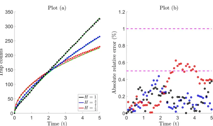
Figure 1. Plot (a) Diffusive flux: Solid curves show the total fluxJ(t)obtained from the diffusion model over time 0<t <5 with analytic solution given by (30), with fixed diffusion constantsD0 =
0.05,D1 = 0.15 and varying Hurst exponentH = 12 (standard diffusion), H = 34 (super-diffusion)
andH =1 (ballistic). The solution is defined over the semi-infinite domain 0< x<∞with initial uniform distributionu(x,t = 0) = U0 = 200 and point trap u(x = 0,t) = 0. Trap counts: Bold
dots plot cumulative trap countsJtfor Brownian motion with total populationN = 1000 recorded
at timest=0, 0.1, 0.2, ..., 5. Discrete time scale parameter defined by combining (25) and (28), that is
σ2(t)≈2(D0+D1t2H−1)∆twithD0,D1,Hgiven above. Each individual executes a total ofS=5000
steps with constant time step increment∆t=0.001 and total timeT =S∆t =5. Individuals initially uniformly distributed X0(n) ∼ U(0,L = 5). Trap installed at positionx = 0 and simulations are conducted with external boundary condition described in §(2.1). Trap counts are replicated and averaged over ten realizations to reduce the effect of stochasticity. Numerical solution: (Green dashed) represent the mean field numerical solution using the method of explicit finite differences. See Appendix A for further details on the numerical scheme. Plot (b) Absolute relative error: A(t) plotted at timest = hk,h= 0.1,k =0, 1, 2, ..., 50, with average ¯A =0.306 (red), 0.157 (blue), 0.167 (black), to illustrate the magnitude of the discrepancy between the analytic solution and trap counts. (For interpretation of the references to colour in this figure legend, and all subsequent figures, the reader is referred to the web version of the article.)
In Figure (1) Plot (a), we find that there is almost identical agreement between trap counts obtained from the Brownian individual based model and mean field diffusion model, as expected from theory. More specifically, it is shown here that the diffusive flux can be used to reproduce trap count patterns for standard diffusionH= 12, super diffusionH= 34and ballistic movementH=1, to a high level of accuracy. Intuitively, we expect that this holds for diffusion coefficients which have a more complicated time-dependency. The diffusion coefficient consists of three unknown parameters, namely;D0,D1andH. In terms of usage, if initial diffusivity can be measured through experiments, then other parameters can be estimated using the tools outlined in [27], i.e by approximating the flux rate in the limitt →0 and relating it to the expected number of individuals trapped after one time step. Note that, since an analytical solution cannot be obtained for the diffusion model (15) over a finite domain, the numerical solution is also shown for consistency. See Appendix A for details on the explicit finite difference scheme used, and how the flux is computed at the trap boundary.
to be effective. The absolute error (relative to the total population) evaluated at discrete timest=hk is defined by,
A(tk) =
|Diffusive flux - Trap counts|
Total population =
|J(hk)−Jhk|
N , k=0, 1, 2, ...,K (31) with time incrementhand total timeT=hK. The errors are then averaged over(K+1)differences,
¯ A(tk) =
1 N(K+1)
K
∑
k=0|J(hk)−Jhk|. (32)
Table 1. Tabulated values of the average absolute relative error ¯Aas defined by (32), to compare the fit between the anomalous diffusion model (30) and trap counts obtained from Brownian motion (see Figure1).
Standard diffusionH=12 Super diffusionH= 34 Ballistic diffusionH=1
Brownian trap counts 0.306 0.157 0.167
Plot (b) illustrates the discrepancy using the absolute error, which lies within 0.6−0.7% of all total trap counts. Theoretically, the Brownian and corresponding diffusion model are equivalent, and the errors can be dismissed as somewhat negligible, partly due to accumulation of small computational errors. We expect this error to tend to zero, with magnitude of stochastic fluctuations decreasing asN−12 in the limitN→∞, [68]. Also, longer time simulations (not shown) demonstrate
that the discrepancy increases as the effect of external boundary encounters is realised. Therefore, we require that the finite domain is large enough, that is LD2 is much larger than the typical characteristic trapping time. The quantified errors in Table1are probably not useful on their own, however, for now they function as benchmark values which indicate an extremely good fit - indicating equivalence. As a general rule of thumb, we classify the level of fit as; equivalent 0< A¯ ≤0.5, good fit 0.5< A¯ ≤1, moderate fit 1<A¯≤1.5 and poor fit ¯A>1.5. These will be useful later as a point of reference, when comparisons are made between various diffusion models, in an attempt to reproduce L´evy trap count data.
4. BM vs LW: Equivalence II
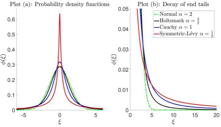
4.1. Stable Laws
In the case of Brownian motion, the step distribution is Normal (2), and the end tails decay exponentially fast (thin tail). A large number of studies have shown that animal movement can follow a more complicated movement pattern where the step distribution decays much slower according to some type of inverse power law (heavy or fat tail), known as L´evy walks [32,44,69]. As a result, individuals have a greater chance of executing ’rare’ large steps, and therefore the properties of the random walk are altered. The biological consequence is such that the overall movement pattern is faster in comparison to what is typically observed in Brownian motion. L´evy walks can be characterized by L´evyα-stable distributions, simply known as stable laws. A distribution is said to be stable if the sum (or, more generally, a linear combination with positive weights) of two independent random variables has the same distribution up to a scaling factor and shift, [70,71]. The mechanisms behind the resulting movement are governed by the step distribution, which is completely described using four parameters, namely, a tail index α ∈ (0, 2], skewness parameter β ∈ [−1, 1], scale parameterγ ∈ (0,∞)and a location parameter δ ∈ R. The asymptotic behaviour of the end tails
is,
whereα ∈ (0, 2]determines the rate at which the tails of the distribution taper off. Forα ≤ 0 the distribution cannot be normalized, and therefore the pdf cannot be defined. For α ≥ 2 the end tails decay sufficiently fast at large|ξ|, ensuring that all moments exist and the central limit theorem (CLT) applies, that is the probability density of the walker after S steps converges to the Normal distribution asS→∞. The generalized central limit theorem (gCLT) states that the sum of identically distributed random variables with distributions having inverse power law tails converges to one of the stable laws, of which the Normal distribution is a special case. For the range 0 < α < 2 the gCLT applies and the condition on the second moment is relaxed, that is; second moments diverge and the tails are asymptotically equivalent to a Pareto law. Since their first introduction, usage of stable laws has been overlooked and somewhat neglected, mainly due to difficulties arising from an infinite variance. However, there are now well developed and readily available algorithms that can be exploited for simulation runs [72,73], and thus stable laws are increasingly being considered, particularly in movement ecology [40].
Stable laws can be parametrized in Z different but equivalent ways, currently there exists at least eleven different variations which has led to much confusion [74,75]. Each type has an advantage over the others and the parameterZ is often chosen based on purpose for use, i.e simulation based studies, data fitting, or study of algebraic/analytic properties. Since our focus is primarily based on obtaining trap counts from simulations, we choose theZ = 0 parametrization and henceforth use this setting. We adopt the notation introduced by [70]; that is the random variableξis drawn from the stable distribution
S(α,β,γ,δ;Z).
Since explicit pdfs are not available for all values ofα∈(0, 2]the distribution is often described in terms of the characteristic function - the inverse Fourier transform of the pdf,
lnEeiωξ=
(
−γα|ω|α1+iβtanαπ2 ·sign(ω)·(|γω|1−α−1)+iδω, α6=1 −γ|ω|
h 1+2iβ
π ·sign(ω)·log|γω|
i
+iδω, α=1 (34) For an isotropic random walk, the pdf of the step distribution is symmetrical and therefore both the skewness and location parameters are fixed withβ= δ= 0. The resulting distribution is known as anα-stable symmetric L´evy distribution, which is then completely characterized solely by the index αand scale parameterγ. For brevity, we adopt the notation
S(α,β=0,γ,δ=0;Z =0) =S(α,γ),
where it is understood that all parameters are zero except α and γ. The resulting characteristic function in (34) reads
Eeiωξ =exp(−γα|ω|α), (35)
which is a useful way to mathematically describe all (symmetric) stable distributions, since a closed form or analytical expression does not exist for all indicesα, with the exception of the Normalα=2 and Cauchyα=1 cases;
Normal ξ∼S(2,γn) φn(ξ) = 1
2γn
√ πexp
− ξ
2
4γ2n
, γn = √σ
2 (36)
Holtsmark ξ∼S
3 2,γh
φh(ξ) Cannot be expressed in closed form (37)
Cauchy ξ∼S(1,γc) φc(ξ) = γc
π(γ2c+ξ2) (38)
Symmetrical-L´evy ξ∼S
1 2,γl
where, the subscriptsn,h,c,lhave been included to distinguish between the different distributions. For the normal distribution,σ is the standard deviation shown in the step distribution (2), withγn defined in this way due to the choice of parametrization. This relation can be easily derived through the characteristic function (35). Note that, some authors use L´evy distribution to refer to stable laws, however, more commonly it refers to α = 12,β = 1 which is a skewed distribution, defined forξ ≥ 0 [70]. Since we consider symmetric distributions i.e. β = 0, we will refer to (39) as the ’Symmetric’-L´evy distribution. In some cases, the pdf can be expressed analytically, even if it cannot be written in closed form e.g the Holtsmark distribution (37) can be written using hyper-geometric functions (if symmetric) or the Whittaker function (if skewed). Also, the Symmetric-L´evy distribution can be expressed in terms of special functions, such as Fresnel integrals [74]. However, these representations are bulky and not useful in the context of this study.
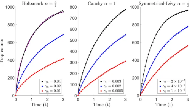
Figure 2.Plot (a): Probability density functionsφ(ξ)for stable laws; Normalα=2, Holtsmarkα= 32,
Cauchyα=1 and Symmetric-L´evyα= 12 with fixed scaling parameterγ=1 chosen for illustrative
purposes (see36-39). Plot (b): Comparison of end tails for differentα, defined by (33)
Figure 2 illustrates pdfs for symmetric stable laws with decay of end tails characterized by different indicesα = 12, 1,32, 2, with faster decay rates asαincreases, and exponential fast decay in the case of the Normal distribution.
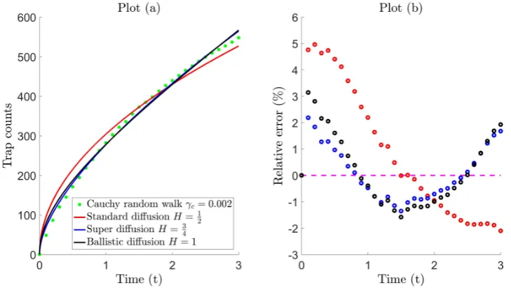
4.2. Equivalence of Trap Counts: Cauchy Walk vs. Diffusion
§4.3), where diffusivity varies continuously with time. On an individual level, the interpretation is such that distinct diffusive rates are adopted, and therefore the model takes into account individual variation. However, at the population level, when rates are aggregated, the movement is governed by time dependent diffusion.
In §3.1it was demonstrated that equivalent trap counts can be obtained for Brownian movement using an anomalous diffusion model (30). Here, we test whether this same model can explain trap counts from non-Brownian movement, with particular interest in the level of discrepancy.
Figure 3. Plot (a):Comparison of trap countsJtfor the Cauchy walkS(α= 1,γc = 0.002)(see38)
against the diffusive fluxJ(t)for anomalous diffusion for the three cases; standard diffusion H = 0.5,{D0,D1}={0.1431, 1.6730}, super-diffusionH =0.75,{D0,D1}={0.7263, 1.1776}and ballistic
diffusionH=1,{D0,D1}={1.228, 0.5844}(see30). Trap counts were averaged over five realizations
to reduce the effect of stochasticity. Total number of individualsN=1000 uniformly distributed over a finite domainL=5 with population densityU0=200. Each individual executes a total ofS=3000
steps with constant time step increment∆t =0.001 and total timeT =S∆t = 3.Plot (b): Relative error (%) measures the discrepancy between trap counts for the random walk and diffusion model defined byJ(t)−Jt
N plotted at timest=0, 0.1, 0.2, ..., 3.
Figure (3) Plot (a) compares trap countsJtfrom the Cauchy walk4against the diffusive fluxJ(t) for exponents; standard diffusion H = 12, super-diffusionH = 34 and ballistic diffusionH = 1. A non-linear curve fitting tool is used to determine the best-fit parametersD0,D1by fitting the analytic solution (30) against trap count recordings in the least squares sense, (see TableB.1for complete list of trap count recordings). Plot (b) illustrates the discrepancy between the trap counts and diffusion model. The relative error is shown (instead of the absolute relative error used previously in Figure1) to distinguish between the time intervals when trap counts are either over or under estimated, here, a positive relative error corresponds to the diffusive flux forming an overestimation, and vice versa. Table (2) quantifies the fit and compares whether the diffusion model can reproduce trap counts as effectively as what was previously seen in the Brownian case (see Figure1).
4 This specific type of random walk is of significant interest in foraging theory since an inverse square power-law distribution
Table 2.Tabulated values of the average absolute relative error ¯Aas defined by (32), to compare the fit between the anomalous diffusion model (30) and trap counts obtained from Brownian motion (see Figure1) and the Cauchy walk (see Figure3).
Standard diffusionH=12 Super diffusionH= 34 Ballistic diffusionH=1
Brownian trap counts 0.306 0.157 0.167
Cauchy trap counts 2.035 0.849 1.120
From Figure3Plot (b) it is clear that standard diffusion fails to predict trap counts adequately, with a maximum relative error of about 5%. This is expected since standard diffusion corresponds to the random walk model with a normal step distribution whose end tails decay exponentially, unlike the Cauchy distribution. On comparison, Table2shows that both Super diffusion and ballistic diffusion provide a good/moderate fitting, respectively. Petrovskiiet al. [26] demonstrated that in the case of some simple diffusion models, such as linear dependency on time D(t) = at+b and its variation D(t) = at+bt13 (a,b constant), both of which constitute ballistic motion, provide a
reasonable fit to trap count data. Figure (3) also confirms a reasonable fit for the ballistic case where the relative error lies within approx. 3%, however, still an evident discrepancy is noticed. Trap counts are much better reproduced by super-diffusion, in this caseH= 34with relative error within approx. 2%. This is somewhat expected, since it is well known that generally, super diffusion has long been acquainted with L´evy walks [41,78]. Despite this promising accuracy, note that the diffusion flux tends to alternate; in the sense that trap counts are overestimated for small time, underestimated for intermediate time and overestimated again on a larger time scale - for both the super diffusive and ballistic case. This phenomena is also realised for other Hurst exponents in the super-diffusive and ballistic regime (simulations not shown here), even when a variety of scale parameters are considered. Although, the accuracy of the matching is somewhat ecologically acceptable in either case, a diffusion coefficient which yields trap counts to a higher level of precision is sought.
In a recent study, Ahmed and Petrovskii [27] demonstrated that the time-dependency of the diffusion coefficient could be inherently more complex than that proposed by anomalous diffusion. Subsequently, a time dependent diffusion model was developed to provide an alternative framework for a Cauchy walk with step distribution (38). In particular, passive trap counts were reproduced effectively and the study indicated that in the case of a Cauchy walk, the problem of trap count interpretation can be addressed with a high precision based on the diffusion equation. However, some drawbacks with this model5 include, firstly; the complicated structure of the diffusion coefficient leads to practicality issues, since it is not expressed in closed form. Secondly; the model consists of multiple unknown parameters with little room for interpretation i.e the ecological significance of parameters or how they relate to the movement pattern is unclear. Finally; the study is constrained to Cauchy walks, and it is not known whether the diffusion model is effective in predicting trap counts for a broader range of tail indices α. With this background, we attempt to address the following: Can trap counts obtained from a system of genuine L´evy walkers be accurately reproduced using the diffusion equation, in particular, with a greater accuracy than what is observed for anomalous diffusion in Figure (3)? If so, what is the structure of the diffusion coefficient and how can the behaviour of the resulting diffusion profiles be explained from an ecological viewpoint in relation to any parameters?
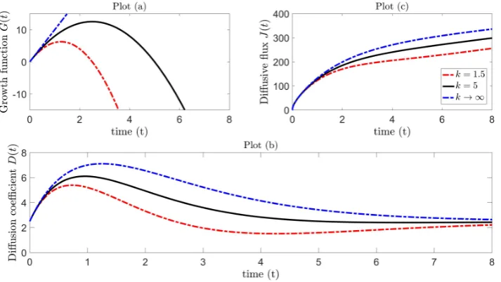
4.3. Proposed Diffusion Coefficient
Observations of trap count patterns (such as those typically observed in Figure3) suggest that the coefficient proposed should consist of some type of growth functionG(t), which should behave
as a controlling mechanism for diffusivity on a short and/or intermediate time scale. In addition to this, a suitable decay function should also be introduced to induce a dampening effect to ensure that trap counts are not overestimated for larger time, typically observed when the movement process grows faster than standard diffusion. Intuitively, we propose the following structure
D(t) = D0 |{z} Initial diffusivity
+ G(t) | {z } Growth function
· e−νt |{z} Exponential
decay
(40)
withG(0) = 0, i.e growth is zero att = 0 so that initial diffusivity is defined as D(0) = D0, with obvious meaning. Here, the growth function is subject to exponential decay causing the diffusivity to be damped over larger times with damping coefficient ν. Subsequently, the diffusivity returns to an initial stateD0 in the large time limit as t → ∞, provided the growth function is not faster than exponential growth, that is limt→∞G(t)e−νt=0. The corresponding diffusive flux for an initial uniform population densityU0across a semi-infinite domainx > 0 with zero density condition at x=0 (described in §3) can be derived using (20), which reads
J(t) =2U0 s
D0t
π +
1 π
Z t
0 G(s)e
−νsds. (41)
A number of possible candidates for the growth function exist in the literature, but are often applied to model population dynamics. Examples of such include; logistic, Gompertz, von Bertalanffy, generalized or hyper-logistic growth [79]. The simplest of these is the logistic type, and an example of application is the Rosenzweig and MacArthur [80] model for predator-prey interactions with logistically growing prey. We propose that the growth function G(t) in (40) grows logistically, as a means to model diffusivity, rather than the typical use of modelling populations, so that
G(t) =D1t
1− t
k
(42)
with corresponding diffusion coefficient
D(t) =D0+D1t
1− t
k
e−νt. (43)
The movement dynamics are then completely governed by set parameters{D0,D1,k,ν}, all positive. This growth function is a parabolic function of time, which increases fromG=0 at timet=0, until a maximumGmax= 14D1kis attained at timet= 2k, and then decreases until the growth diminishes, i.e G=0 at timet=k. The corresponding diffusion coefficient is still valid for negative growth over the intervalk<t<t∗providedD(t)>0, wheret∗is a solution of lnD1(t∗−k)−νt∗ =lnD0k. For fixed
D1, the value of kcontrols the maximum growth capacity and also determines the instant in time when growth alternates from positive to negative. In the special case, for sufficiently small time with largek, the term kt in (43) is negligible and the growth function is approximately linearG(t) ≈ D1t, and in the limiting case ask→∞,
G(t) =D1t (44)
with corresponding diffusion coefficient,
which now depends on three parameters{D0,D1,ν}. The corresponding diffusive flux can be derived for the logistic model (42) from (41), which results in
Model 1: J(t) =2√U0 π
D0t+ D1
ν2
1−(1+νt)e−νt+ D1
kν3
h
(ν2t2+2νt+2)e−νt−2
i
1 2
(46)
and simplifies to
Model 2: J(t) = 2√U0 π
D0t+
D1
ν2
1−(1+νt)e−νt
12
(47)
in the reduced linear case (44). Henceforth, we will refer to this as Model 1 & 2, respectively.
Figure 4. Plot (a) Growth function: LogisticG(t) = D1t 1−ktwhich reduces to linear growth
G(t) =D1task→ ∞. Plot (b) Diffusion coefficient: D(t) = D0+D1t 1−tk
e−νtwhich reduces toD(t) = D0+D1te−νt ask → ∞. Parameter values (chosen for illustrative purposes): D0 =2.5
D1=10,ν=0.8 with different valuesk=1.5, 5, including the limiting casek→∞.Plot (c):Diffusive
flux given by (46-47).
Figure4Plot (a) illustrates the logistic growth function as a parabolic profile for different values ofk, with linear growth ask→∞. Figure4Plot (b) shows how the diffusion coefficient behaves for particular parameter values. In ecological terms, the mechanistic process is such that insect diffusivity increases from the initial valueD0 until maximum diffusivityDmaxis attained at timet = 2k+ 1ν−
k 2
q 1+ 4
(kν)2. We presume that this increase in diffusion rate can induce faster movement, which can
be comparable (at some level) to the pattern inherent in L´evy walks. Following this, the diffusivity begins to decrease until it reaches a minimum levelDminat timet = k2+ ν1+k2q1+(k4
ν)2, and then asymptotically approaches the initial state D0 in the large time limit. In the special case of linear growth function, insect diffusivity reachesDmax = D0+ D1
eν at timet =
1
ν with no subsequent local minimum, and same asymptotic behaviour ast → ∞. Figure4 Plot (c) illustrates the flux for each corresponding diffusion coefficient in Plot (b), it is precisely these diffusion Models 1 & 2 (46-47) which will be tested in §4.4against L´evy trap count data.
4.4. Reproducing Lévy Trap counts using Diffusion
laws, defined in (37 -39). Also, the assumptions that the walk is uncorrelated and unbiased in a homogeneous environment still apply. In a system of N individuals executing a L´evy walk, the position of thenthindividual at the(i+1)thstep can be described by
X(n)i+1=Xi(n)+ξ, i=0, 1, ...,S, n=1, 2, ...,N, ξ∼S(α,γ), α∈(0, 2). (48) The trap count is expected to grow faster with time, compared to what is usually recorded for Brownian movement. This is due to the frequency of long jumps increasing, and therefore the contribution from remote parts of the population to the trap count also increases. For our purposes, we simulate trap counts for the tail indicesα= 32, 1,12, referring to the Holtsmark (37), Cauchy (38) and Symmetric-L´evy (39) distributions, previously introduced in §4.1. The movement dynamics are completely governed by the scale parametersγh,γc,γl. Although, comparing random walks prior to simulation runs can reveal information on parameter selection [81] (also see §2.2), for our purposes it suffices to arbitrarily select three distinct scale parameters for each case i.e. γh = 0.01, 0.02, 0.04, γc = 0.0005, 0.002, 0.003 andγl = 1×10⁻⁶, 4×10⁻⁶, 2×10⁻⁵. Here, parameters are chosen so that trap count data is obtained with reasonable level of variation (see TableB.1). The diffusive flux curves J(t)given by Model 1 (46) & Model 2 (47) are then fitted (in the least squares sense) against these trap counts using a non-linear curve fitting tool and best-fit parameters are estimated, listed in Table3.
Figure 5. Simulation details:In accordance with the simulation setting in §2.1,N=1000 individuals are initially uniformly distributed along a 1D spatial domain 0 < x < L = 5. After one time step
∆t=0.001, each individual executes a single step, with subsequent position defined by the recurrence relation (48). A total number ofs=3000 steps are executed, with total time of exposureT=st=3. Prior to the simulation run, an impermeable external boundary is installed atx = 5 ensuring that no individual can escape or enter the system at this end (no-migration/immigration), by forcing the condition; ifX(in) > 5 at any instant in time then Xi(n) = 5. The point trap at x = 0 functions
in the following way; ifX(in) < 0 at any instant in time then the individual is removed from the system and the accumulated trap count increases by one. Consequently, the number of individuals in the population decrease as time flows, and an increasing stochastic trap count trajectory is formed. Trap counts: Bold dots depict cumulative trap counts Jt recorded for the cases (a) Holtsmark, (b)
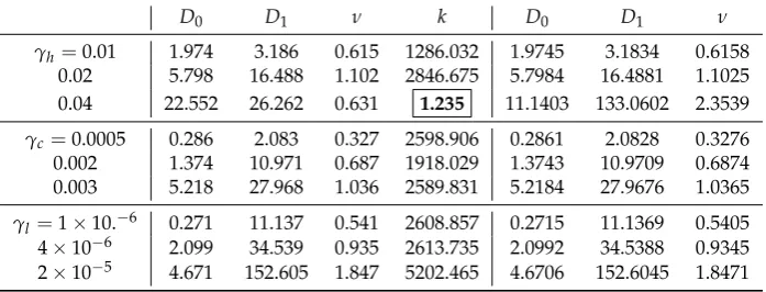
Table 3.Best-fit parameters using a non-linear curve fitting tool (in the least squares sense) by fitting Model 1 (46) and Model 2 (47) against cumulative trap counts (see Table B.1for complete list of recordings). The diffusion coefficients in Figure6are those plotted with highlighted parameters in the Table below.
D0 D1 ν k D0 D1 ν
γh=0.01 1.974 3.186 0.615 1286.032 1.9745 3.1834 0.6158
0.02 5.798 16.488 1.102 2846.675 5.7984 16.4881 1.1025 0.04 22.552 26.262 0.631 1.235 11.1403 133.0602 2.3539
γc=0.0005 0.286 2.083 0.327 2598.906 0.2861 2.0828 0.3276
0.002 1.374 10.971 0.687 1918.029 1.3743 10.9709 0.6874 0.003 5.218 27.968 1.036 2589.831 5.2184 27.9676 1.0365
γl=1×10.−6 0.271 11.137 0.541 2608.857 0.2715 11.1369 0.5405
4×10⁻⁶ 2.099 34.539 0.935 2613.735 2.0992 34.5388 0.9345 2×10⁻⁵ 4.671 152.605 1.847 5202.465 4.6706 152.6045 1.8471
Figure5illustrates the fitting between the diffusive flux J(t) and L´evy trap count data Jt, for the Holtsmarkα = 32, Cauchyα = 1 and symmetric-L´evyα = 12 distributions, respectively. Model 2 is shown and found to form an almost identical fit, with the exception of the Holtsmark case with γh = 0.04. In this special case, we find that Model 2 eventually overestimates trap counts, which is more apparent for largerγh. Here, we find that Model 1 forms a better fit and this can also be realised on inspection of best fit parameters in Table3. The parameterkis significant (compare boxed value with otherk), and therefore the term kt behaves as some type of correction term which slows the diffusivity rate. The corresponding growth function is of logistic type, with diffusion coefficient D(t) = D0+D1t 1−kt
e−νt. In all other cases, kis relatively large, and therefore on a short time scale the term tk in this diffusion coefficient is negligible. As a result, the growth function is then approximately linear and Model 1 reduces to Model 2 with diffusion coefficientD(t) =D0+D1te−νt.
Figure 6.Diffusion coefficients given by (45) for Model 2 (red, blue black curves) with listed best-fit parameters in Table3. Diffusion coefficient given by (43) for Model 1 shown only in Plot (a) (dashed curve).
the initial value for larger time (where the latter is not typically essential as the interest is on short time dynamics). In the special case, seen in Plot (a), the rate of decay for Model 2 (black curve) is slower than required, resulting in larger diffusivity and explains the overestimation previously observed in Figure5Plot (a) for the Holtsmark case withγh =0.04. On comparing the diffusion coefficients for both models, we find that trap counts are better estimated using a profile with larger initial diffusivity, smaller peak and faster decay (see dashed curve).
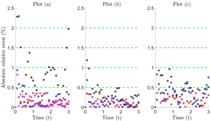
Figure 7.Absolute relative error between trap counts and diffusive flux for the cases (a) Holtsmark, (b) Cauchy and (c) Symmetric-L´evy. Each colour corresponds to those cases with scale parameters shown in Figure5.
Table 4.Tabulated values of the average absolute relative error ¯Aas defined by (32), to compare the fit between models 1 (46) and 2 (47) and trap counts. ¯Ais also included for the anomalous diffusion model, see Figure3and Table2.
Diffusion γh=0.01 0.02 0.04 γc=0.0005 0.002 0.003 γl=10−6 4×10⁻⁶ 2×10⁻⁵
StandardH=12 2.035
SuperH=34 0.849
BallisticH=1 1.120
Model 1 (46) 0.139
Model 2 (47) 0.162 0.198 0.839 0.123 0.135 0.299 0.194 0.370 0.394
5. Discussion
The biological basis behind time dependent diffusion, and how this is linked to the type of mechanisms involved has not been clearly understood [51]. Here, the parameters introduced have ecological significance with obvious meaning, in the sense that they are not all arbitrary and are related to the underlying movement dynamics. One possible explanation of the type of diffusive pattern seen in Figure6can be arrived at through the concept of differential energetics [82–84]. If an individual executes a large step, then this will incur higher energy costs than a small step, so energy expenditure for different step lengths is a given. In relation to basic individual traits, such as body mass, a heavier body requires a larger force and a larger energy expense to change direction or execute a larger step. Therefore, it may be expected that the frequency of moving long distances is lower for heavier individuals. Also, for those individuals that do prefer to take large steps, this could possibly induce larger rest pauses contributing towards intermittent behaviour [85], from which decrease in the rate of diffusivity can be explained. On the other hand, the mechanisms behind the movement behaviour could involve a degree of spatial synchronisation of individual variation. In the case of movement with a physiological origin, this could result from a diffusivity distribution as indicated byPetrovskii and Morozov[47] or alternatively, even time dependent diffusion. Also, with reference to behavioural effects, a sudden event may trigger change in behaviour in one individual that results in swarming behaviour, leading to a change at the population level [86]. It must also be realised that the build up of insect population and following changes in diffusivity can also be a result of transient environmental factors, e.g temperature [87], as sudden temperature changes can excite movement or even lead to erratic behaviour. If one or more of these factors can bring about diffusive movement varying with time, then as a consequence, the pattern produced by an insect population performing Brownian motion may be indistinguishable from the pattern produced by insects performing L´evy walks. Altogether, it seems that identifying a genuine L´evy walk may be more challenging than previously thought. In light of this, it is not surprising that the L´evy or diffusion controversy has been persistent, with strong evidences arguing for either side - in this study, we have demonstrated that both sides are somewhat equivalent, at least in the context of trapping.
On a final note, we would like to mention some limitations and suggest possible further research directions. Although, this study is purely theoretical and attempts to answer some important issues in movement ecology, it is limited to the 1D spatial scale. In a more practical scenario, it would be interesting to see a similar study in a more realistic 2D domain, which would be more relevant to field studies with trapping of walking/crawling insects [12,28]. The problem would then have enhanced complexity due to the introduction of a single trap of different possible shapes and sizes. The movement pattern would then be altered, as the effects of trap and field boundaries are realised by enforcing a confined or restricted space [59]. In particular, interest would lie in how the time dependent diffusion model could be further refined in order to produce trap counts to a high level of accuracy within these different geometries. The diffusion model can then be checked and tested for good agreement against insect trap counts in the real field, given that there is evidence of L´evy type movement beforehand. Developing a corresponding model in 2D would be the next obvious step to take.
corresponding theory is largely absent. In this case, the convenient mathematical framework would consist of advection-diffusion equations, where possibly, a time dependent diffusivity may be used.
6. Concluding Remarks
In this paper, we show that the diffusion coefficients (43) and the reduced version (45) can be incorporated into a time-dependent diffusion model, which can then be used to predict, almost identically, trap counts from a system of individuals who undergo a L´evy walk. Moreover, we show that this can be achieved for a broad range of L´evy tail indices. Also, we find that these proposed diffusion models are much more accurate and effective when compared to super diffusion. Alongside the development of the models, we explore the biological basis for time-dependent diffusion in more detail, and interpret parameters in relation to diffusive patterns. We argue that, if these inherently different movement models yield almost identical trap counts, then how important is the movement pattern in the context of trapping? This study suggests that the movement pattern is not that important after all, rather emphasis should be on the ecological context, at least in integrated pest monitoring programmes.
Acknowledgments:The authors are thankful to Rod Blackshaw and Carly Benefer (Plymouth, UK) for fruitful discussions relating to the biological interpretation in the discussion, end of §5. We also thank Katriona Shea (Penn State University, USA) for her brief comments on the main message of the paper. D.A.A. gratefully acknowledges the support given by Prince Mohammad Bin Fahd University (KSA) through the Phase II grant, which was essential for the completion of this work. P.F.C.T. and S.V.P. gratefully acknowledge support from The Royal Society (UK) through the grant no. NF161377. P.F.C.T. was also supported by Sao Paulo Research Foundation (FAPESP–Brazil), grant no. 2013/07476-0, and partially supported by CAPES, Brazil.
Author Contributions: D.A.A. provided the theoretical results, conducted the simulations and wrote majority of the paper. S.V.P. reviewed the paper and contributed by providing a detailed revision, which substantially improved the manuscript. P.F.C.T. wrote §2.2and provided the details therein.
Conflicts of Interest:The authors declare no conflict of interest.
Appendix A. Mean field numerical solution
Consider the 1D diffusion equation for the population density u(x,t) with time dependent diffusion coefficient D = D(t) over the finite domain 0 < x < L, with initial uniform density u(x,t = 0) = U0. The boundary conditions include the zero density conditionu(x = 0,t) = 0 at the trap boundary and no-flux condition∂u(L∂x,t) =0 at the external boundary. To summarise,
∂u
∂t =D(t) ∂2u
∂x2, u(x,t=0) =U0, u(x=0,t) =0,
∂u(L,t)
∂x =0 (A.1)
An analytical solution can only be derived for the system (A.1) over the semi-infinite domainL=∞, previously demonstrated in §3. In the case of finite L, a numerical solution can be sought using the method of explicit finite differences [92,93] by introducing a uniform computational grid. We discretize the spatial and temporal scales,
tk+1=k∆t, k=0, 1, 2, ... (A.2)
x1=0, xn+1=xn+∆x, n=1, 2, ...,N (A.3) with constant time∆tand spatial∆xincrements. For brevity, using the notation
u(xn,tk) =ukn, u(xn,tk+∆t) =uk+n 1 and u(xn+∆x,tk) =ukn+1 we can approximate the partial derivatives as
∂u ∂t ≈
uk+n 1−ukn ∆t ,
∂2u ∂x2 ≈
ukn+1−2ukn+ukn−1
Here we have used a forward difference for∂u
∂t and a central difference for ∂2u
∂x2. The numerical scheme is said to be explicit since the solution at the(k+1)st time step, namelyuk+n 1, is given explicitly in terms of the valuesukn from the previous time layertk. Discretizing the diffusion equation in (A.1) and rearranging, we obtain the recurrence relation
uk+n 1=ukn+
D(k∆t)∆t (∆x)2 (u
k
n+1−2ukn+ukn−1). (A.5) The theoretical approximation related to this numerical scheme isO(∆x2+∆t), and in the case of short time dynamics of trap counts, we are interested in the solution for small time t, where we can assume that the approximation errorO(∆t)is negligible. The reader is redirected to [94] for a discussion on local/global truncation and round-off errors. The spatial-temporal increments must also satisfy the Courant-Friedrichs-Lewy condition
D(k∆t)∆t (∆x)2 <
1
2. (A.6)
to ensure stability. Other numerical schemes such as the method of implicit finite differences relax this condition, however, since our interest lies in calculating the flux through the trap boundary for small time, the explicit scheme suffices with simpler computation. The initial condition can be written as u0n = u(xn,t0) = U0, and the discretization of the trap boundary reads uk1 = 0 with the no-flux conditionukN+1 = ukNat the external boundary. The flux j(t)through the trap boundary at timetis given byj(t) =−D∂u(x=0,t)
∂x . To compute this we approximate the derivative ∂u ∂x ≈
ukn+1−ukn
∆x , and at the trap locationx = 0 corresponding to grid noden = 1, this reduces to ∂u(x=0,t)
∂x ≈
uk2−uk1
∆x . Therefore, the flux through the boundary at timetkis given by
j(tk) =D(k∆t)
|uk 2−u1k|
∆x (A.7)
Here, we take the absolute value instead of omitting the ’−’ sign which would be required since the flux is in the opposite direction of the positivex-axis. A linear approximation is used in (A.7), alternatively, a more accurate way to compute the flux uses a quadratic polynomial [55], which yields an error in line with the numerical scheme i.eO(∆x2). For our simulations the linear approximation suffices, and we choose the spatial step∆xto be sufficiently small to ensure that any accumulated errors are negligible. The cumulative flux passing through the trap boundary between timestk and tk+1can be computed as
Jk,k+1=j(tk)∆t=
∆tD(k∆t)|u2k−uk1|
∆x (A.8)
The cumulative fluxJk+1from timet>0 is then computed by summing
Jk+1= Jk+∆tD(k∆t)|u k 2−uk1|
∆x (A.9)
Appendix B. Trap count recordings
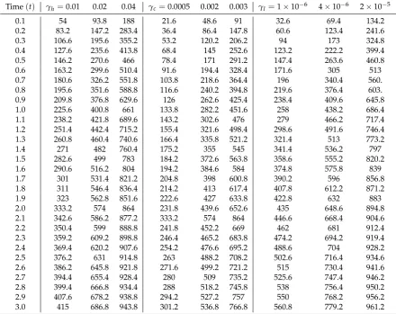
Table B.1. Trap count recordings for the cases (a) HoltsmarkS(α = 32,γh), (b) CauchyS(α=1,γc),
(c) Symmetric-L´evyS(α=12,γl), with tail exponentαand scale parameterγ. Simulation details with
all parameter values are given in the caption of Figure5.
Time(t) γh=0.01 0.02 0.04 γc=0.0005 0.002 0.003 γl=1×10⁻⁶ 4×10⁻⁶ 2×10⁻⁵
0.1 54 93.8 188 21.6 48.6 91 32.6 69.4 134.2
0.2 83.2 147.2 283.4 36.4 86.4 147.8 60.6 123.4 241.6
0.3 106.6 195.6 355.2 53.2 120.2 206.2 94 173 324.8
0.4 127.6 235.6 413.8 68.4 145 252.6 123.2 222.2 399.4
0.5 146.2 270.6 466 78.4 171 291.2 147.4 263.6 460.8
0.6 163.2 299.6 510.4 91.6 194.4 328.4 171.6 305 513
0.7 180.6 326.2 551.8 103.8 218.6 364.4 196 340.4 560.
0.8 195.6 351.6 588.8 116.6 240.2 394.8 219.6 376.4 603. 0.9 209.8 376.8 629.6 126 262.6 425.4 238.4 409.6 645.8
1.0 225.6 400.8 661 133.8 282.2 451.6 258 438.2 686.4
1.1 238.2 421.8 689.6 143.2 302.6 476 279 466.2 717.4
1.2 251.4 442.4 715.2 155.4 321.6 498.4 298.6 491.6 746.4 1.3 260.8 460.4 740.6 166.4 335.8 521.2 321.4 513 773.2
1.4 271 482 760.4 175.2 355 545 341.4 536.2 797
1.5 282.6 499 783 184.2 372.6 563.8 358.6 555.2 820.2
1.6 290.6 516.2 804 194.2 384.6 584 374.8 575.8 839
1.7 301 531.4 821.2 204.8 398 600.8 390.2 596 856.8
1.8 311 546.4 836.4 214.2 413 617.4 407.8 612.2 871.2
1.9 323 562.8 851.6 222.6 427 633.8 422.8 632 883
2.0 333.2 574 864 231.8 439.6 652.6 435 648.6 894.8
2.1 342.6 586.2 877.2 333.2 574 864 446.6 668.4 904.6
2.2 350.4 599 888.8 241.8 452.2 669 462 681 912.4
2.3 359.2 609.2 898.8 246.4 465.2 683.8 474.2 694.2 919.4 2.4 369.4 620.2 907.6 254.2 476.6 695.2 488.6 704 928.2
2.5 376.2 631 914.8 263 488.2 708.2 502.6 716.4 934.6
2.6 386.2 645.8 921.8 271.6 499.2 721.2 515 730.4 941.6
2.7 394.4 655.4 928.4 280 509 735.2 525.6 747.4 946.2
2.8 399.4 666.8 934.4 288 518.2 745.8 538 756.4 950.2
2.9 407.6 678.2 938.8 294.2 527.2 757 550 768.2 956.2
References
1. Burn, A.Integrated pest management.; New York: Academic Press, 1987.
2. Kogan, M. Integrated pest management: historical perspectives and contemporary developments. Annu. Rev. Entomol.1998,43, 243 – 70.
3. MEA. Ecosystems and human well-being: Biodiversity synthesis of the millennium ecosystem assessment. Washington, DC: World Resources Institute; 2005 Millennium Ecosystem Assessment2005. 4. Cardinale, B.; Duffy, J.; Gonzalez, A.; Hooper, D.; Perrings, C.; Venail, P.; Narwani, A.; Mace, G.; Tilman,
D.; Wardle, D.; Kinzig, A.; Daily, G.; Loreau, M.; Grace, J.; Larigauderie, A.; Srivastava, D.; Naeem, S. Biodiversity loss and its impact on humanity. Nature2012,486, 59 – 67.
5. Ahmed, D.; van Bodegom, P.; Tukker, A. Evaluation and Selection of Functional Diversity Metrics for Life Cycle Assessments. Int. J. Life Cycle Assess.2018. Under review.
6. Pimentel, D.; Greiner, A. Environmental and socio-economic costs of pesticide use. In: Pimentel, D, editor. Techniques for reducing pesticide use: economic and environmental benefits.; New York: John Wiley and Sons, 1997.
7. Alavanja, M.; Ross, M.; Bonner, M. Increased cancer burden among pesticide applicators and others due to pesticide exposure. C.A. Cancer J. Clin.2013,62, 120 – 42.
8. Bourguet, D.; Guillemaud, T. Sustainable Agriculture Reviews; Vol. 19,The Hidden and External Costs of Pesticide Use., Springer, 2016. pages 35 – 120.
9. Pimentel, D. Amounts of pesticides reaching target pests: environmental impacts and ethics. J. Agric. Environ. Ethics1995,8, 17 – 29.
10. Alyokhin, A.; Baker, M.; Mota-Sanchez, D.; Dively, G.; Grafius, E. Colorado potato beetle resistance to insecticides.Am. J. Potato Res.2008,85, 395 – 413.
11. Sohrabi, F.; Shishehbor, P.; Saber, M.; Mosaddegh, M. Lethal and sub-lethal effects of imidacloprid and buprofezin on the sweet potato whitefly parasitoid Eretmocerus mundus (Hymenoptera: Aphelinidae). Crop. Prot.2013,45, 98 – 103.
12. Petrovskii, S.; Ahmed, D.; Blackshaw, R. Estimating Insect Population Density. Ecol. Complex2012, 10, 69–82.
13. Holland, J.M.; Perry, J.N.; Winder, L. The within-field spatial and temporal distribution of arthropods in winter wheat. Bull. Entomol. Res.1999,89, 499 – 513.
14. Ferguson, A.W.; Klukowski, Z.; Walczak, B.; Perry, J.N.; Mugglestone, M.A.; Clark, S.J.; Williams, I. The spatio-temporal distribution of adult Ceutorhynchus assimilis in a crop of winter oilseed rape in relation to the distribution of their larvae and that of the parasitoid Trichomalus perfectus. Entomol. Exp. Appl. 2000,95, 161 – 171.
15. Alexander, C.J.; Holland, J.M.; Winder, L.; Woolley, C.; Perry, J.N. Performance of sampling strategies in the presence of known spatial patterns.Ann. Appl. Biol.2005,146, 361 – 370.
16. Byers, J.A.; Anderbrant, O.; Lofqvist, J. Effective attraction radius: a method for comparing species attractants and determining densities of flying insects.J. Chem. Ecol.1989,15, 749 – 765.
17. Raworth, D.A.; Choi, M. Determining numbers of active carabid beetles per unit area from pitfall-trap data. Entomol. Exp. Appl.2001,98, 95 – 108.
18. Turchin, P.Quantitative analysis of movement: measuring and modelling population redistribution in animals and plants; Sinauer Associates, 1998.
19. Okubo, A.; Levin, S.Diffusion and ecological problems: modern perspectives; Springer, New York, 2001. 20. Lewis, M.; Maini, P.; Petrovskii, S.Dispersal, individual movement and spatial ecology.; Springer, Berlin., 2013. 21. Levin, S.; Cohen, D.; Hastings, A. Dispersal strategies in patchy environments. Theor. Popul. Biol. 1984,
26, 165 – 180.
22. Reichenbach, T.; Mobilia, M.; Frey, E. Mobility promotes and jeopardizes biodiversity in rock-paper-scissors games.Nature2007,448, 1046 – 1049.
23. Hengeveld, R.Dynamics of biological invasions.; Chapman and Hall, London, 1989.
24. Shigesada, N.; Kawasaki, K.Biological invasions: theory and practice; Oxford University press, 1997. 25. Petrovskii, S.; Brian, L.Exactly solvable models of biological invasion; Chapman and Hall/CRC, 2006. 26. Petrovskii, S.; Petrovskaya, N.; Bearup, D. Multiscale approach to pest insect monitoring: Random walks,