A Numerical Study of Renormalization Group Transformations
on Multiscale Lattices
JiqunTu1,and RobertMawhinney1
1Department of Physics, Columbia University, New York, NY 10027, USA
Abstract.The RBC and UKQCD Collaborations have shown that light hadron masses and meson decay constants measured on 2+1 flavor Mobius DWF ensembles generated with the Iwasaki gauge action and a dislocation suppressing determinant ratio (DSDR) term show few percentO(a2) scaling violations for ensembles witha−1 = 1 GeV. We call this combination the ID+MDWF action and this scaling implies that, to a good ap-proximation, these ensembles lie on a renormalization group trajectory, where the form of the action is unchanged and only the bare parameters need to be tuned to stay on the trajectory. Here we investigate whether a single-step APE-like blocking kernel can reproduce this trajectory and test its accuracy via measurements of the light hadron spec-trum and non-perturbative renormalization. As we report, we find close matching to the renormalization group trajectory from this simple blocking kernel.
1 Introduction
The RBC and UKQCD Collaborations have recently generated several 2+1 flavor ensembles with the ID+MDWF action at three different lattice spacings and various values for the quark masses. Global fits to these ensembles and ensembles at weaker coupling generated with the Iwasaki gauge action were performed, using fit anzätz from SU(2) chiral perturbation theory, including analytic expansions for variations in the strange quark mass around its physical value [1]. A typical fit takes the form of (equation (9) in [1])
X(m,a2)X0(1+f(m)+cXa2), (1) whereXare observables,X0is the chiral and continuum limit andf(m) is the chiral perturbation theory or analytic function giving the quark mass dependence. We observe that on ID+MDWF ensembles thesecX coefficients are typically∼0.02 GeV2forX = fπ andX = fK.1 This leads to percent scale scaling errors on oura−1=1 GeV ensembles.
While measurements of more complicated quantities such as BK and the ∆I = 3/2 K → ππ
matrix elements are underway, these small scaling errors imply that theories with the ID+DSDR action lie, to a good approximation, on a renormalization group (RG) trajectory, up to a few percent discrepancy. While knowing a good approximation to an RG trajectory might help in producing a multiscale evolution algorithm, it is also of interest to investigate whether a numerically tractable
e-mail: [email protected]
1mπ,mKandm
blocking kernel, whichcarriesthe transformation on this RG trajectory, exists. This latter topic is the subject of this report.
We start with the pair of ID+MDWF ensembles shown in Table1. These havemπ ∼300 MeV, physical kaon masses, lattice spacings that differ by a factor of 2 and essentially the same physical volume. We refer to these as the coarse and fine ensembles, with actionsSc andSf respectively, which are both ID+MDWF actions. From the table one can see that they have the same physics at the 5% level and this agreement could be made closer by more careful tuning of the input parameters, but this precision is accurate enough for this study.
In general, ablocking kernel G[Uc,Uf] [2] will map a fine configuration with linksUf to a coarse configuration with linksUc. The action for the blocked coarse lattice,Sbc[Uc] is given by
e−Sb c[Uc]∝
[dUf]e−Sf[Uf]G[Uc,Uf]. (2)
Here we seek a numerically tractable blocking kernel that produces a blocked coarse lattice, with ac-tionSb
c[Uc], that is as close as possible toSc[Uc]. We will work with a coarse and a fine ensemble whose lattice spacings differ by a factor of essentially 2. Since we will not have a closed form ex-pression forSb
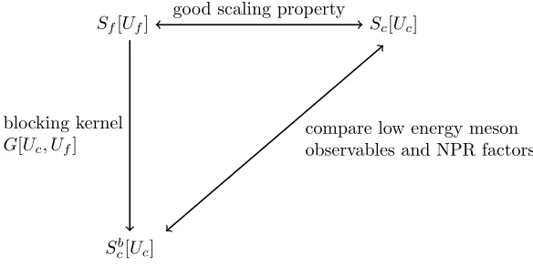
c[Uc], we will use measurements of physical quantities on the blocked, coarse lattice as a measure of the agreement between it and the original coarse action ensemble. Figure1gives a diagram showing our strategy.
Sf[Uf] good scaling property Sc[Uc]
blocking kernel
G[Uc, Uf]
Sb c[Uc]
compare low energy meson observables and NPR factors
Figure 1.Strategy of our comparison.
A general blocking kernelG[Uc,Uf] is a functional defined as a product of delta functions, with arguments which are SU(3) links from both the coarse and fine lattice, denoted byUcandUf, respec-tively.
G[Uc,Uf]=
x,µ
δUc(x, µ)−gb[Uf;x, µ]
. (3)
blocking kernel, whichcarriesthe transformation on this RG trajectory, exists. This latter topic is the subject of this report.
We start with the pair of ID+MDWF ensembles shown in Table1. These havemπ ∼300 MeV, physical kaon masses, lattice spacings that differ by a factor of 2 and essentially the same physical volume. We refer to these as the coarse and fine ensembles, with actionsScandSf respectively, which are both ID+MDWF actions. From the table one can see that they have the same physics at the 5% level and this agreement could be made closer by more careful tuning of the input parameters, but this precision is accurate enough for this study.
In general, ablocking kernel G[Uc,Uf] [2] will map a fine configuration with linksUf to a coarse configuration with linksUc. The action for the blocked coarse lattice,Sbc[Uc] is given by
e−Sb c[Uc] ∝
[dUf]e−Sf[Uf]G[Uc,Uf]. (2)
Here we seek a numerically tractable blocking kernel that produces a blocked coarse lattice, with ac-tionSb
c[Uc], that is as close as possible toSc[Uc]. We will work with a coarse and a fine ensemble whose lattice spacings differ by a factor of essentially 2. Since we will not have a closed form ex-pression forSb
c[Uc], we will use measurements of physical quantities on the blocked, coarse lattice as a measure of the agreement between it and the original coarse action ensemble. Figure1gives a diagram showing our strategy.
Sf[Uf] good scaling property Sc[Uc]
blocking kernel
G[Uc, Uf]
Sb c[Uc]
compare low energy meson observables and NPR factors
Figure 1.Strategy of our comparison.
A general blocking kernelG[Uc,Uf] is a functional defined as a product of delta functions, with arguments which are SU(3) links from both the coarse and fine lattice, denoted byUcandUf, respec-tively.
G[Uc,Uf]=
x,µ
δUc(x, µ)−gb[Uf;x, µ]
. (3)
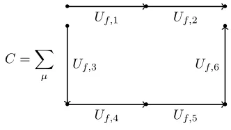
Heregb[Uf;x, µ] is a function which determines the blocking kernel. Figure2shows the blocking kernel we experiment with in this paper. The kernel is similar to the well known APE smearing method, except that it produces a coarse ensemble link from a pair of links in the fine lattice, plus staples spanning the two fine-lattice links.αis an adjustable parameter which we will determine later.
• Uf,1 • Uf,2 • → •
gb[Uf] =P[(1−α)Uf,1Uf,2+αC/6] • C= µ • Uf,3 • Uf,4 • Uf,5 •• Uf,6 •
Figure 2.Single-step APE-like blocking kernel.
2 Numerical Methods
We start by generating a coarse and fine ensemble with the ID+MDWF actions, whose lattice spacings differ by a factor of 2. As mentioned, the RBC and UKQCD Collaborations have seen smallO(a2) errors for this action. To make our studies easier, we use smaller volumes and targetmπ ∼300 MeV. Table1shows the results for basic observables on these ensembles. The lattice spacing comes from √t
0 andw0 measurements and we have used the global fits results[1] to determine the input quark masses. Our input quark masses could be refined to reduce the 2−7% errors seen in the table to perhaps below 3%, but we believe this agreement is accurate enough for our current purposes. Both ensembles have physical spatial volumes of about (2.4 fm)3.
Oc Of % diff.
size 123×32×12 243×64×12 −
β 1.633 1.943 −
aml 0.008521 0.000787 −
amh 0.065073 0.019896 −
a−1[GeV] 1.015(16) 2.001(18) −
amres 0.007439(86) 0.004522(12) −
mπ[MeV] 307(5) 300(3) 2.3
mK[MeV] 506(8) 491(5) 3.0
mΩ[MeV] 1652(27) 1557(71) 5.9
fπ[MeV] 147(2) 138(2) 6.3
fK[MeV] 166(3) 155(2) 6.8
Table 1.Parameters and measurements of the fine and coarse lattices. The lattice spacing comes from √t0and
w0measurements.
between the coarse and fine ensemble, there is some RG blocking of the fine lattice which will remain in the ID+MDWF plane; our task is to see if we can get a good approximation to this RG blocking
from our single-step APE-like blocking kernel.
β, ml, mh,· · · •
•
•
•
Sf[Uf]
Sc[Uc] Sb
c[Uc]
G[Uc, Uf]
compare
space of all possible actionsS[U]
hyperplane of actions consist of
only ID+MDWF termsS[U;β, ml, mh]
Figure 3.Illustration of the comparison. A general blocking kernelG[Uc,Uf] will lead the fine lattice action out
of the hyperplane of actions consist of only ID+MDWF terms, as shown by the dashed line. There exist some
blocking kernel which will keep the fine action in the ID+MDWF hyperplane, giving the perfect scaling between
the coarse and fine ensemble.
A simple minded way to proceed would be to choose a value forα, block the fine ensemble and measure physics observables on the resulting blocked, coarse ensemble and compare with the coarse ensemble. We believe a better way to do this is to utilize the demon algorithm[3]. Applying this algorithm to the lattices in an ensemble, one can find the coefficients (couplings) for any term in the
action which could have appeared in the generation of the ensemble, or in an effective representation of
the action. Here we are generating ensembles including fermions and we can use the demon algorithm to find an action, expressed as a sum of Wilson loops, that would produce the same ensemble.
Given a configuration generated according to some action, possibly including fermions, we can introduce a series ofdemonvariables to determine the underliningβiin an expansion of the action in
terms of a set of Wilson loops, denoted bySi. These terms can be the plaquette(P), rectangular(R),
chair loop(C), twist loop(T), etc.
[DU]
i
[dEi] exp
−
i
(βiSi[U]+βiEi) .
The update scheme for the demon consists of two parts: 1. updateU’s only.
2. updateU’s andEi’s at the same time while keepingSi+Eiconstant. In this case the accept/reject
step does not require knowledge ofβi’s.
Since the integration of theEi’s factorizes we can measure the average value of them and probe the
underlyingβi’s through the relation
Ei= 1
βi −
Emax
tanh(βiEmax).
We apply the demon algorithm on the configurations generated bySc[Uc]2, and configurations
generated bySb
c[Uc] with differentα’s. The result is shown in table2. We choose to useα=0.688, which gives the closest match for the coefficient of the plaquette,βP, between the coarse and blocked
coarse ensembles. For this choice ofα, we also see that the coefficient ofβR for the coarse and
blocked-coarse ensembles differ by 50%, although both are small. No further matching is possible
with our single parameter blocking kernel, so we will work with this value ofα.
ensemble βP βR βC βT
Sc[Uc] 2.035(36) −0.1018(33) −0.0026(30) −0.0006(30) α=0.0 0.617(11) 0.0491(33) 0.0032(32) 0.0010(32)
α=0.5 1.478(35) −0.0020(44) 0.0043(42) −0.0016(43)
α=0.688 2.030(28) −0.1522(30) −0.0021(24) 0.0038(24) α=0.7 2.069(33) −0.1589(33) 0.0009(27) −0.0003(27)
Table 2.Results of the demon algorithm applied to blocked coarse ensembles, produced with various values for
the blocking parameter,α. The results of applying the demon algorithm to the coarse lattice are given in the first
row.
3 Results
We can now compare physical observables on the coarse and blocked coarse lattices. For pure gauge quantities, we use the same observable to do the measurement on both ensembles. For fermionic observables, we need to calculate propagators on the blocked coarse lattice, which means we need to choose which gauge fields and quark masses to use in the MDWF Dirac operator. To the extent that the blocked coarse and coarse lattices are equivalent, we can use the same quark masses in both cases. Since the MDWF residual mass may be different between the two cases, we will present results with
the total quark masses the same,i.e.the input quark mass plus the residual mass.
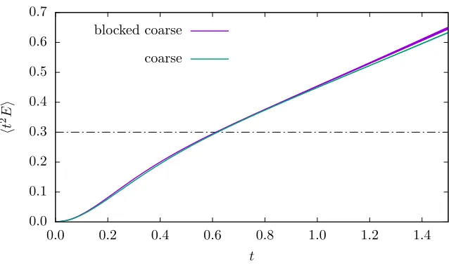
Turning first to the Wilson flow, Figure 4 shows the results on the coarse and blocked coarse lattices. One sees very good agreement between the two ensembles up to very large flow times.
We have also measured some light hadron masses and meson decay constants on the two ensem-bles and Table3shows the results. The differences are at the 1−3% level between the coarse and
blocked coarse lattices. We note that for the coarse ensemble, we know the sea quark mass and use this mass for the measurements (they are unitary). For the blocked coarse ensemble we do not know the sea quark mass, but use the same total quark mass as the coarse ensemble. To do this, we have to measure the residual mass on the blocked coarse ensemble, which we do by choosing the fifth di-mension,Ls, to be 12, as it is on the coarse ensemble. (The residual mass does depend modestly on
2Fermion determinants are in principle sums of Wilson loops. Our inclusion of only 4 types of Wilson loops is justified by
t
2E
t
blocked coarse coarse
0.0 0.1 0.2 0.3 0.4 0.5 0.6 0.7
0.0 0.2 0.4 0.6 0.8 1.0 1.2 1.4
Figure 4.Wilson flow of the coarse and blocked coarse ensembles.
the quark mass used in the measurement. This is generally a small effect and we do not correct for it here.) Our condition on the quark masses is
am
l+amrescoarse=aml+amresblocked coarse. (4)
Oc Obc % diff.
size 123×32×12 123×32×12 −
β 1.633 − −
aml 0.008521∗ 0.007494 −
amh 0.065073∗ 0.064150 −
a−1[GeV] 1.015(16) 1.010(16) 0.5(2.3)
amres 0.007439(86) 0.00847(21) −
amπ 0.3026(13) 0.3050(35) 0.8(1.2)
amK 0.4982(11) 0.5018(25) 0.7(0.5)
amΩ 1.628(10) 1.668(25) 2.4(1.6)
a fπ 0.14472(64) 0.1491(10) 2.9(0.8)
a fK 0.16333(47) 0.16723(85) 2.3(0.6)
Table 3.Spectrum measurements on coarse and blocked coarse lattices. See section3for the choice of valence quark mass on the blocked coarse ensemble. Again the lattice spacing comes from √t0andw0measurements.
t
2 E
t
blocked coarse coarse
0.0 0.1 0.2 0.3 0.4 0.5 0.6 0.7
0.0 0.2 0.4 0.6 0.8 1.0 1.2 1.4
Figure 4.Wilson flow of the coarse and blocked coarse ensembles.
the quark mass used in the measurement. This is generally a small effect and we do not correct for it here.) Our condition on the quark masses is
am
l+amrescoarse=aml+amresblocked coarse. (4)
Oc Obc % diff.
size 123×32×12 123×32×12 −
β 1.633 − −
aml 0.008521∗ 0.007494 −
amh 0.065073∗ 0.064150 −
a−1[GeV] 1.015(16) 1.010(16) 0.5(2.3)
amres 0.007439(86) 0.00847(21) −
amπ 0.3026(13) 0.3050(35) 0.8(1.2)
amK 0.4982(11) 0.5018(25) 0.7(0.5)
amΩ 1.628(10) 1.668(25) 2.4(1.6)
a fπ 0.14472(64) 0.1491(10) 2.9(0.8)
a fK 0.16333(47) 0.16723(85) 2.3(0.6)
Table 3.Spectrum measurements on coarse and blocked coarse lattices. See section3for the choice of valence quark mass on the blocked coarse ensemble. Again the lattice spacing comes from √t0andw0measurements.
It is worth pointing out that by using the same total quark mass on the coarse and blocked coarse ensembles, and finding the same physical hadron masses, we are implicitly seeing that the
renormal-ization factors for the quarks are the same on these two ensembles. This is a statement not just about the equivalence of long distance physics on both ensembles, but also includes at least some of the short distance physics.
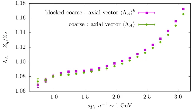
To pursue this question further, we have also measured the non-perturbative renormalization (NPR) factors on the coarse and blocked coarse ensembles using the RI/SMOM scheme[4]. We find generally very good agreement between the two measurements, with differences of∼1% over a range of renormalization scales. Figure5shows the NPR Z-factor,ZA, for the local axial vector current, as a function of the renormalization scale on the two ensembles. On sees that the differences ofZA at high energy scales (compared to the lattice spacing) are around 1%. Given the matching between low energy measurements, this further shows that the two actions,Sc[Uc] andSb
c[Uc] can be considered as the same action, up to an accuracy of a few percent.
1.06 1.08 1.10 1.12 1.14 1.16 1.18
1.0 1.5 2.0 2.5 3.0 ΛA
=
Zq
/Z
A
ap, a−1∼1 GeV blocked coarse : axial vectorΛAb
coarse : axial vectorΛA
Figure 5.Non-perturbative renormalization factorZAof the coarse and blocked coarse ensembles.
4 Conclusion
We have generated a matched pair of lattices, coarse and fine, with 300 MeV pions and lattice spac-ings differing by a factor of 2, using the ID+MDWF actions. Using the demon algorithm, a simple APE-like blocking kernel is tuned to block the fine lattice into a blocked coarse lattice. Measurements of physical hadron masses, meson decay constants and the Wilson flow scale were made on the coarse and blocked coarse ensembles. The results show only a few percent difference. We have also measured renormalization factors using non-perturbative renormalization on the coarse and blocked-coarse en-sembles and find good agreement between them. The good scaling properties of the ID+MDWF action imply that the coarse and fine lattices are related, to a good approximation, by an RG blocking transformation. We have found that a simple, numerically tractable, blocking kernel provides a good RG blocking transformation between these lattices.
Beyond understanding the properties of these ensembles better, we were also motivated to un-dertake this study to think about ways of improving evolution algorithms. IfSc[Uc] andSb
very nearly equal, we could imagine evolving both coarse and fine lattice concurrently, by writing the following:
O=
[dUf]e−Sf[Uf]O[Uf]
[dUf]e−Sf[Uf]
(5)
=
[dUc]G[Uc,Uf][dUf]e−Sf[Uf]O[Uf]
[dUc]G[Uc,Uf][dUf]e−Sf[Uf]
(6)
=
[dUc]e−Sb c[Uc]
[dUf]e−S f[U f]G[Uc,Uf]O[Uf]
[dUf]e−S f[U f]G[Uc,Uf]
[dUc]e−Sb
c[Uc] (7)
In the second line we have inserted a [dUc]G[Uc,Uf] factor which is a constant when integrated over
Ucand the third line uses the definition of the blocked action, equation (2).
Equation (7) states that we will get the same value for observables if we performconstrained
Monte Carlo on the fine lattice in the background of coarse lattices generated with the actionSb c[Uc]. This is a further step from what is described in [5]: this is a multiscaleevolutionalgorithm, rather than just a multiscalethermalizationalgorithm. The coarse (free) evolution and the fine constrained evolution can be performed successively with no additional thermalization needed. The coarse evolu-tion gives us short decorrelaevolu-tion length for various quantities including the global topological charge and the fine evolution fills in the much wanted short scale details, which enable the inclusion of heavy quarks.
Unfortunately, an exact evolution algorithm requires thatSc[Uc] andSb
c[Uc] agree much more accurately than we have seen here. A viable algorithm would need a correction step or a reweighting factor, or other improvements, to facilitate such a multiscale Monte Carlo.
5 Acknowledgement
We would like to thank all members of the RBC and UCQCD Collaborations for their help and comments, especially Norman Christ, Christopher Kelly, David Murphy and Chulwoo Jung. The simulations reported here were done on the BG/Q Computers of the RIKEN-BNL Research Center and Brookhaven National Laboratory. The authors are supported in part by the U.S. Department of Energy (DOE) Grant No. DE-SC0011941.
References
[1] P.A. Boyle, N.H. Christ, N. Garron, C. Jung, A. Jüttner, C. Kelly, R.D. Mawhinney, G. McGlynn, D.J. Murphy, S. Ohta et al., Phys. Rev. D93, 054502 (2016),1511.01950
[2] Y. Iwasaki, UTHEP118, 20 (1983),1111.7054
[3] M. Hasenbusch, K. Pinn, C. Wieczerkowski, Phys. Lett. B338, 308 (1994),9406019
[4] Y. Aoki, P.A. Boyle, N.H. Christ, C. Dawson, M.A. Donnellan, T. Izubuchi, A. Jüttner, S. Li, R.D. Mawhinney, J. Noaki et al., Phys. Rev. D78, 1 (2008),0712.1061
![Figure 3. Illustration of the comparison. A general blocking kernel G[Uc, U f ] will lead the fine lattice action outof the hyperplane of actions consist of only ID+MDWF terms, as shown by the dashed line](https://thumb-us.123doks.com/thumbv2/123dok_us/8052697.1341795/4.482.96.320.150.313/figure-illustration-comparison-blocking-lattice-hyperplane-actions-consist.webp)