FOAM: Searching for Hardware-Optimal SPN Structures and
Components with a Fair Comparison
Khoongming Khoo1, Thomas Peyrin2, Axel Y. Poschmann3, and Huihui Yap1
1
DSO National Laboratories, 20 Science Park Drive, Singapore 118230.
{kkhoongm,yhuihui}@dso.org.sg
2 SPMS, Nanyang Technological University, Singapore.
3 NXP Semiconductors
Abstract. In this article, we propose a new comparison metric, the figure of adversarial merit (FOAM), which combines the inherent security provided by cryptographic structures and components with their im-plementation properties. To the best of our knowledge, this is the first such metric proposed to ensure a fairer comparison of cryptographic designs. We then apply this new metric to meaningful use cases by study-ing Substitution-Permutation Network permutations that are suited for hardware implementations, and we provide new results on hardware-friendly cryptographic building blocks. For practical reasons, we considered linear and differential attacks and we restricted ourselves to fully serial and round-based implementations. We explore several design strategies, from the geometry of the internal state to the size of the S-box, the field size of the diffusion layer or even the irreducible polynomial defining the finite field. We finally test all possible strategies to provide designers an exhaustive approach in building hardware-friendly cryptographic primitives (according to area or FOAM metrics), also introducing a model for predicting the hardware performance of round-based or serial-based implementations. In particular, we exhibit new diffusion matrices (circulant or serial) that are surprisingly more efficient than the current best known, such as the ones used inAES,LEDand
PHOTON.
Key words:SPN, lightweight cryptography, figure of adversarial merit, diffusion matrices.
1 Introduction
RFID is a rising technology that is likely to be widely deployed in many different situations of everyday life, leading to new security challenges that the cryptography community has to handle. Significant ad-vances in this area have already been obtained. In particular, many lightweight block ciphers [10,12,17,22] have recently been proposed, and designing such ciphers is not an easy task as showed by the numerous candidates that eventually got broken. Moreover, it is interesting to note that in most privacy-preserving RFID protocols proposed [3,18,19] a hash function is required, and since a hash function can be easily built from a block cipher (for example with the Davies-Meyer mode) or a permutation (for example with the sponge construction [9]), a crucial question for the researchers is how to design a hardware efficient permutation (that can later be utilized to build a hash function and/or a block cipher).
Hardware efficiency can have very different meanings depending on the utilization scenario targeted by the designer. For example, a classical metric is to estimate the minimum silicon area required by the primitive to perform the cryptographic operations. This, of course, depends on the parameters of the function itself (the area is highly dependent on the amount of memory required) and most lightweight block ciphers have a rather small block size of 64 bits. It is to be noted that the area is usually not directly linked to the security of a primitive, as adding extra rounds will have an impact on the throughput of the implementation, but only a very limited one concerning the area (we assumed that the function has no weakness that is independent of the number of rounds). Area and other metrics such as throughput, latency or power dissipation can be traded-off for one another, making the comparison between different primitives difficult. In the direction of fairer comparisons of hardware implementations of cryptographic primitives, Bogdanov et al. [11] introduced the efficiency metric throughput/area in order to take in account these tradeoffs. However, the possibility of trading off throughput for power was not taken in account and Badel et al. [4] proposed instead a figure of merit, defined as FOM = throughput/area2.
c
However, as of today, no metric takes in account the inherent security of a building block, therefore making it hard to compare for example two diffusion matrices that have different area footprint and different branching number.
The construction of good diffusion matrices has always been an important research topic in cryp-tography, equally important as the search for good confusion functions. TheAES [15] for example uses a 4×4 matrix with elements in GF(28). This matrix is Maximum Distance Separable (MDS), which
means that it has a branching number of 5, optimal for a 4×4 matrix. However, this security feature comes at a cost that computations inGF(28) might not be the best choice for some hardware purposes, even though special care has been taken by the designers to choose a circulant matrix instantiated with lightweight coefficient (i.e. low Hamming weight coefficients, such as 0x01, 0x02 and 0x03). Recently, Guoet al.[16,17] described a new type of diffusion matrix, so-called serial, that trades more clock cycles in the execution for a smaller area. This idea was later extended to the use of linear Feistel-like struc-tures or Linear Feedback Shift Registers (LFSR) to build the diffusion matrix [21,23]. On the opposite side, PRESENT [10] uses a simple bit permutation layer, the real diffusion coming in fact directly from the S-box application. The advantage being of course that a bit permutation layer is basically free in a hardware implementation. Now, one may ask the following question: what is better when the goal is to maximize some hardware metric, a very weak diffusion matrix with a low area footprint, or a strong diffusion matrix but requiring more silicon to be performed?
More generally, many different trade-offs exist when building anAES-like Substitution-Permutation Network (SPN) primitive, such as the general geometry (number of lines and columns), what size of S-box, what type of matrix, with what branching number, in what finite field, with which irreducible polynomial, etc. When a cryptographer would like to design a permutation with a specific hardware efficiency metric in mind, it is not trivial for him to make the best construction choices directly. Since implementing many different trade-offs is very time consuming, he will have to rely on his own intuition when picking the basic building blocks and choosing the general structure of the primitive, therefore accepting that his final design might not be optimal.
Our contributions. In this article, we study the problem of designing hardware efficient permutations for lightweight symmetric key cryptography purposes, and we propose new promising diffusion matrices as building blocks. We first explain in Section2 the family of functions that we will study, namelyAES -like SPN permutations, and we describe a new generalized diffusion layer (i.e. theShiftRows function inAES), that allows a provable optimal diffusion even for non-square internal state matrices. Then, we introduce in Section3a new metric, thefigure of adversarial merit (FOAM), that for the first time takes into account the inherent security provided by the primitive. We then explain in Section 4 the various SPN design tradeoffs that we will consider for our comparisons, such as the geometry of the SPN, the S-box size, the type of matrix (circulant or serial), the field size for the diffusion or even the irreducible polynomial. The goal being that the designer only has to input the type of implementation (round and/or serial) and the size of the permutation he would like to build, and he can directly get the SPN structure and its internal components that are the best suited for him. We study in Section5 the security of the AES-like SPN permutations by only taking in account simple linear/differential attacks. We then describe how one can estimate the hardware implementations efficiency in Section 6 and in particular the non trivial task of estimating the area consumption induced by the control logic. Moreover, we show that in some situations, a coefficient rewrapping trick can be used to significantly improve the efficiency of a diffusion matrix. We chose to focus our work on designing permutations only since many cryptographic primitives can be built from them. Therefore, we will not cover other components such as key schedule for a block cipher, or message expansion for a hash function. Moreover, due to the obviously vast amount of implementation trade-offs, we restricted ourselves to the two most important cases: fully serialized and round-based.
2 Generic SPN with generalized optimal diffusion
In this section, we describe the family of AES-like SPN functions we are considering. Our scope is quite classical, but we propose a new generalized diffusion layer (i.e. the ShiftRows function in AES), that allows an optimal diffusion even for non-square internal state matrices.
2.1 Extended AES-like permutations
An n-bit AES-like SPN permutation transforms an r ×c array of s-bit cells (n = r×c×s). During one round, each cell is first transformed by an s-bit S-box (similar to the AES SubBytes operation). Then each r-cell column is transformed by an r×r diffusion matrix (similar to the AES MixColumns operation), followed by an optimal diffusion which permutes the c cells of each row to provide further mixing (similar to theAES ShiftRowsoperation). Finally, an (r×c)-cell constant is XORred to complete a round transformation (in a block-cipher design, this phase is a subkey addition, but we will not consider key-schedules in this article). Note that in AES, we have a square array r = c = 4 and cell size s= 8-bit. The diffusion matrix is usually defined over the finite field GF(2s) because of the s-bit cell size. Sometimes, we might actually use a smaller subfield of sizeGF(2i), i divides s, in order to define the diffusion matrix. This framework captures many known ciphers such asAES,PRESENT,LED, etc.
In this paper, a cell is called differentially (resp. linearly) active if its value (resp. mask value) is non-zero in a differential (resp. linear) attack. The differential branch number of a diffusion matrix is the minimum number of differentially active input and output cells (among all non-zero inputs). The notion of linear branch number is similar, except that we consider the transpose of the diffusion matrix instead. From this point onwards, we will not distinguish between differential and linear branch number unless necessary. That is, if it is stated that a matrix has branch number, say, 3, we mean that both the differential and linear branch number are 3. The maximum branch number for anr by r diffusion matrix isr+ 1, and a matrix which achieves this optimal branch number is called Maximum Distance Separable (MDS). If the diffusion matrix has branch numberr, then it is called almost-MDS.
2.2 The generalized optimal diffusion
In this section, we generalize the concept of optimal diffusion [15] for non-square state array. This has been done already whenr < c with a security bound equivalent to the case where r =c (square array) [15]. Whenr > cand cdividesr, a simple generalization has been proposed in [13] where a 4-round security bound is proven when the diffusion matrix is MDS. In this section, we propose a generalized optimal diffusion for the caser > cwhere cmay not divider and the diffusion matrix may not be MDS, i.e. for all branch numberB ≤r+ 1.
An example of optimal diffusion is theShiftRowsoperation ofAESwhich helps to diffuse the effect of theAES SubBytesandMixColumnsoperation over 32-bit to the whole 128-bit block. TheAES ShiftRows transforms a 4×4 byte-array by rotating row r to the left by r bytes, for r = 0,1,2,3. The effect of ShiftRows is that each byte of an input column is mapped to a different output column. This is captured by the concept of optimal diffusion (another example is the ArrayTranspose map of the SQUAREcipher [14]).
Definition 1. For an r-by-r cell-array, the optimal diffusion map is a cell-permutation that maps each cell of an input column to a different output column.
However, the optimal diffusion only applies for r×ccell array where r ≤c. When r > c, there are not enough output columns c to map each of the r cells of an input column. Thus, we extend a new concept from [13] called Generalized Optimal Diffusion (GOD) forr×c cell-array when r > c, which we describe below. Our strategy is to distribute the cells of an input column as uniformly as possible to each output column.
Note that here, without loss of generality, we apply the permutation operations from right-to-left, i.e.SC(SubCells) is first applied, followed byMC(MixColumn) and then the optimal diffusion.
The Generalized Optimal Diffusion (GOD) defined in [13] applies only whenris a multiplec. Here, we deinfeGODfor any
Definition 2. For an r ×c cell-array, a generalized optimal diffusion is a cell-permutation such that looking at any r-cell column:
1. dr/ce input cells are mapped to each of (r mod c) output columns. 2. br/cc input cells are mapped to each of c−(r mod c) output columns.
Example 1. Consider r = 5, c = 3. For each input column of 5 cells,d5/3e= 2 input cells are mapped to each of (5 mod 3) = 2 columns. b5/3c= 1 input cell is mapped to 3−(5 mod 3) = 1 column. One example is given by the transform of the following arrays:
a1 b1 c1
a2 b2 c2
a3 b3 c3
a4 b4 c4
a5 b5 c5
maps to
a1 b1 c1
a2 b2 c2
c3 a3 b3
c4 a4 b4
b5 c5 a5
Theorem 1. Consider a 4-round AES-like SPN as follows (omitting the constant addition since it has no effect on our reasoning):
GOD◦MC◦SC◦GOD◦MC◦SC◦GOD◦MC◦SC◦GOD◦MC◦SC,
where
1. SubCells is a nonlinear substitution layer with r×c s-bit S-boxes acting in parallel.
2. MixColumnsis a layer of cparallel MixColumn transforms each mappingr cells to r cells with branch number B, i.e. MixColumns(x1, . . . ,xc) = (MixColumn(x1), . . . ,MixColumn(xc)), each xi
correspond-ing to a column of r cells.
3. GOD(generalized optimal diffusion) is as defined above which distributes thercells of an input column almost uniformly to coutput columns.
Then the number of active S-boxes over1 and 2 rounds are at least 1 and B respectively. For 4 rounds it is at leastB×B0 where B0 = max{2;x+y} and:
y= min{2×(r modc));bB/dr/cec} x= d(B− dr/ce ×y)/br/cce
We provide the proof of this theorem in Appendix A.1. We note that it is tight in the sense that it naturally provides a 4 round path that corresponds to a “luckiest” scenario for the attacker, which involves the minimum number of active Super-Sboxes (the (c×s)-bit S-boxes composed of twoSubCells layers surrounding oneMixColumns).
Let us look at an application example of Theorem 1 to derive the number of active S-boxes of an AES-like SPN structure, which cannot be deduced by the known results of [13,15]. Consider an SPN structure with state size 24-cell, the diffusion matrices being an 8×8 matrix with branch number 7, i.e.
r= 8,c= 3 andB = 7. By Theorem1, we havey= 2 andx= 1, therefore B0 = max{2;x+y}= 3 and there areB×B0 = 7×3 = 21 active S-boxes guaranteed over 4 rounds of this 24-cell SPN structure.
As a corollary, we explore the cases when the formula for the number of active S-boxes over 4 rounds can be simplified (the proof is given in AppendixA.2).
Corollary 1. In Theorem 1, we have the following special cases:
1. If c > r, then the number of active S-boxes over four rounds is at least B2 (known result from [15]). 2. If c divides r and B = r+ 1, i.e. MixColumn is MDS, then the number of active S-boxes over four
rounds is at least (r+ 1)×(c+ 1)(known result from [13]).
3 FOAM: Figure Of Adversarial Merit
As explained in the introduction, the various trade-offs inherent in any design of a cryptographic primitive make a fair and consistent comparison of software and hardware implementations thereof a challenging task. For hardware implementations exist a few metrics, like theArea-Time (AT) product, which multi-plies the area inGate Equivalents (GE) occupied by the design with the number of clock cycles required (the smaller the number, the more efficient is the design). Closely related is thehardware efficiency [11], which divides the throughput at a given frequency by the area (hence the greater the number, the bet-ter the design). In order to also address the area-power trade-off, [4] proposed a new Figure of Merit (FOM): throughput divided by the area squared. The latter two metrics are frequency dependent, which can complicate comparisons.
We propose a new metric called Figure of Adversarial Merit (FOAM) in order to resolve the afore-mentioned shortcomings. It is defined as
F OAM(x) = 1
S(x)×A2
where S(x) and A are basically equivalent to special definitions of speed and area, respectively. More precisely, S(x) denotes the speed of the cipher based on the number of rounds required to achieve a certain security x against some set of attacks (in this article, we will later restrict ourselves to simple differential/linear attacks). For a round-based permutation, it is defined asS(x) =p(x)×twhere p(x) represents the number of rounds required to achieve security x, and t the number of clock cycles to perform one round. Moreover, for SPN-based primitives, we decompose the area requirementsAinto six parts: the intermediate state memory cost Cmem, the S-boxes implementation cost Csbox, the diffusion
matrix implementation cost Cdif f, the constant addition Ccst, the control logic cost Clog, and the IO
logic costCio:
F OAM(x) = 1
S(x)×A2 =
1
p(x)×t×(Cmem+Csbox+Cdif f +Ccst+Clog+Cio)2
This FOAM metric will be useful to compare different design strategies, different building blocks (such as diffusion matrices) with a simple value computation. Even better, we would like to roughly compare all these possible design trade-offs without having the hassle to implement all of them: in Section6 we will detail how to estimate these six subparts of the area cost and the number t of clock cycles required to perform one round. The value p(x) can be deduced by the number of active S-boxes proven in Theorem 1 and the S-box cryptographic properties (see Section 5). Note that in the rest of the paper, we consider that the security aimed by the designer is equal to the permutation size, i.e. we are aiming at a security of 2n computations (thusp(x) =p(2n)).
4 Trade-offs considered
In this section, we explain all the various trade-offs we will consider when building an AES-like SPN permutation. The goal being that a designer specifies a permutation bitsizen, the metric he would like to maximize (area, FOAM), the degree up to which serial or round-based implementations are important, and he directly obtains the best parameters to build his permutation.
The S-box. One of the first choice of the designer is the size of the S-box, and we will consider two possible trade-offs: s = 4 and s = 8. Note that, for simplicity, we will consider that the S-box chosen has perfect differential and linear properties relative to its size (one could further extend the trade-offs to non-optimal but smaller S-boxes, but the search space being very broad we leave this as an open problem).
Diffusion matrix field size. The designer can choose the field size 2iin which the matrix computations will take place. The classical case, like in AES, being that the field size for the diffusion matrix is the same as the S-box. However, depending on the diffusion matrices available, it might be worth considering designs with thinner diffusion layers but repeated several times. For example, in the case ofAES, instead of theMixColumnsmatrix one could use a 4×4 diffusion matrix onGF(24) applied two times (one time on the 4 MSB and one time on the 4 LSB of the 8-bit cells in theAEScolumn). Overall, we will cover a scope from binary matrices (in GF(2)) up to matrices on the same field size as the S-box (inGF(2s)).
Irreducible polynomial for the diffusion matrix field. Once the field size 2i is fixed, the designer can choose the irreducible polynomial defining the field. Fori = 1 and i = 2 only a single polynomial exists, while fori= 4 at most 3 choices are possible (α4+α+ 1,α4+α3+ 1 andα4+α3+α2+α+ 1). For thei = 8 case, many polynomials are possible (this was already observed by [5]), thus in order to focus the search space we will only consider the irreducible polynomial used inAES(α8+α4+α3+α+ 1) and inWHIRLPOOL hash function [7] (α8+α4+α3+α2+ 1).
Type of diffusion matrix. The designer can choose what type of matrix he will implement, the two main hardware-friendly types being circulant or serial. In the circulant case, the designer picks r
coefficientsZ = (Z0, . . . , Zr−1) and the matrixZ is defined as
Z0 Z1 Z2 . . . Zr−2 Zr−1
Zr−1 Z0 Z1 . . . Zr−3 Zr−2
Zr−2 Zr−1 Z0 . . . Zr−4 Zr−3
. . . .
. . . .
Z1 Z2 Z3 . . . Zr−1 Z0
In the serial case, the designer picksr coefficients Z = (Z0, . . . , Zr−1) and the matrixZ is defined as
0 1 0 0 . . 0 0
0 0 1 0 . . 0 0
0 0 0 1 . . 0 0
. . . .
. . . .
0 0 0 0 . . 0 1
Z0 Z1 Z2 . . . Zr−2 Zr−1
r
The matrix therefore takesr operations to be computed.
Branching number of the diffusion matrix. In general, implementing a matrix with very good diffusion property will cost more area and/or cycles than a weak one. For example, theAESmatrix has ideal MDS diffusion property, but certainly requires more area to implement than a simple binary matrix with weaker properties. Since the former is bigger but stronger and the latter is smaller and weaker, it is not clear which alternative will lead to the best FOAM. Therefore, the designer can choose between a wide range of possibilities concerning the branching numberB of the diffusion matrix, fromB = 3 to
B=r+ 1 (MDS).
5 Security assessment of AES-like primitives
The FOAM metric takes into account the security of the permutation with regards to simple differen-tial/linear attacks. We would like to evaluate this security for the AES-like SPN permutations we are considering. Theorem 1 gives us the minimal number of active S-boxes for a given number of rounds,
and knowing the S-box cryptographic properties we can compute the maximum differential and linear characteristic probabilities of our generic SPN ciphers easily. In other words, we can easily compute the number of roundsp(x) =p(2n) required to achieve the aimed security 2n.
As stated before, for simplicity, in the rest of this article we will consider that the S-boxes have perfect differential and linear properties: for a 4-bit S-box the maximum differential and linear characteristic probabilities are 2−2 (e.g. PRESENT S-box), while for a 8-bit S-box the maximum differential and linear characteristic probabilities are 2−6 (e.g. AES S-box). Of course, one can extend the trade-off by considering other S-boxes, that might require a smaller area, but will have worse security properties.
We reuse the example from Section2.2(i.e. SPN structure with state size 24-cell, the diffusion matrix being a 8×8 matrix with branch number 7) as an illustration. Previously, we know from Theorem 1 that there are at least 21 active boxes over 4 rounds of this SPN permutation. Suppose that 8-bit S-boxes (i.e.s= 8) having maximum differential and linear probabilities 2−6 are used. Then the maximum differential and linear characteristic probabilities over four rounds are upper-bounded by (2−6)21= 2−126. We are aware that other attacks rather than simple differential/linear might exist, some perhaps much more complex and powerful (it would be interesting to give some generic description of various attacks like impossible differential attack, boomerang attack, etc. only using the parameters of theAES-like SPN permutation). However, our goal here is not to fully specify a permutation, but it is to compare many trade-offs and design strategies that will lead to good hardware performances. Therefore, we emphasize that the number of roundsp(x) is of course not the number of rounds that should be chosen by a designer. This number should be carefully chosen after thorough cryptanalysis work on the entire primitive. Yet, we believe that this simple differential/linear criterion is a quite accurate way to compare the security of variousAES-like SPN permutations.
6 Implementations in ASIC
In this section, we introduce some notation before we present formulas to estimate serialized and round-based implementations (we restricted ourselves to these two important practical cases due to the obvi-ously vast amount of implementation trade-offs). Please note that all estimates have to be seen aslower bounds, as we use scan flip-flops, and consider neither reset nor I/O requirements, which can significantly impact the area count in practice. We argue that those requirements –though very important in practice– are highly application specific, and thus need to be determined on a case by case basis. In practice, a higher throughout can be achieved by using pipelining techniques to reduce the critical path at the cost of additional area. As this design goal is, again, highly application specific and FOAM is designed to be frequency independent, we have not considered it in our analysis.
We have estimated all serial architectures with the single optimization goal of minimal area in mind. In practice, some design decisions will most likely use another trade-off point more in favor of smaller time and larger area. To reflect this, we have estimated all round-based architectures optimized for maximum FOAM.
The table below provides an overview over the hardware building blocks we used, their notation and typical area requirements for a UMC 180 nm technology. In addition, we denoteithe exponent for the fieldGF(2i).
Notation Description GE
DF F 1-input flip-flop 4.67
SF F 2-input flip-flop 6
M U X 2-input multiplexer 2.33
Notation Description GE
XOR 2-input exclusive Or 2.67
SB4 4 x 4 S-box (PRESENT) 22
SB8 8 x 8 S-box (AES) 233
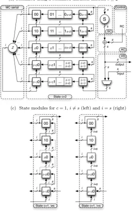
In this section, we give more details about the ASIC implementation estimates given in Section6. A general serialized architectures using a serial diffusion matrix is depicted in Figure1a, while Figure 1b shows the circulant diffusion matrix module. In the special case of c = 1 the state module can be simplified to one of the two the architectures shown in Figure1c, dependent whetheri6=s(left) ori=s
(right). Finally, Figure1d depicts a round-based architecture.
(a) Serialized using a serialized diffusion matrix,c≥2
00 01 0(c-2) 0(c-1)
10 11 1(c-2) 1(c-1)
(i)0 (i)1 (i)(c-2) (i)(c-1)
(r-2)0 (r-2)1 ((c-2r-2)) ((r-2c-1))
s s s ... ... ... ...
(r-1)0 (r-1)1 ((c-2r-1)) ((r-1c-1))
input ... Z RC S s s s s output
State c≧2
SC Control i MC serial s s s ... ... s AC s I/O s i i i i i s s s s i i i i i
(b) Circulant diffusion matrix
Z MC circulant ... ... i i i i i i i i
(c) State modules forc= 1,i6=s(left) andi=s(right)
00
10
(i)0
(r-2)0
(r-1)0
State c=1, i≠s i i i i s s s s i i i i i i s 00 10 (i)0 (r-2)0 (r-1)0
State c=1, i=s i=s s i i i i i i i=s i=s i=s s s (d) Round-based AC SC MC GOD n=s*r*c n n n n n output input n n
Fig. 1: Hardware architectures.
6.1 Serial architectures
Memory cost. The memory is arranged in an r×c array of s-bit cells. In case c ≥ 2 the two outer columns need to be 2-input flip-flopsSF F, while 1-input flip-flopsDF F suffice for the remaining c−2 internal columns. In casec = 1 it depends whether i6= s or i= s. In the former case the whole state consists of 2-input flip-flops, while in the latter case it suffices to use 1-input flip-flops for the upperr−1 rows and only use 2-input flip-flops for the last row.
Cmem=
s·(r− bsic)·SF F +bsics·DF F , c= 1 2·s·r·SF F +s·r·(c−2)·DF F , c≥2
S-boxes cost. We use the S-boxes of AES and PRESENT to estimate the area for 8-bit and 4-bit S-boxes, respectively. In a UMC 180 nm technology they requireSB8 = 233 GE andSB4 = 22 GE.
Csbox=
SB4, s= 4
SB8, s= 8
Once one column has been computed, all columns are rotated by one column to the left and the next column can be processed. In case a circulant matrix is used, additional temporary storage of s×r−i
1-input flip-flops are required before the result is fed back to the leftmost column. Then all columns are rotated by one column to the left. One additionali-bit multiplexer is required.
Cdif f =
A·XOR ,for serial mat.
A·XOR+ (s·r−i)·DF F +i·M U X ,for circulant mat.
Constant addition cost. To add a constant sXOR gates are required.
Ccst=s·XOR
Control logic cost. A particular challenge is to estimate the control logic Clog required for a given
architecture. Our estimates contain four parts: three countersar (rows),ac(columns), and ap (rounds);
the finite state machineb; clock gating logiccg; and other combinational logicoc. The area for counters is mainly determined by the storage required for the minimal number of bits, some simple (e.g. NOT, NAND, NOR) feedback function and at least a 1-bit MUX. In total we estimate the area for any such counter to beax =DF F× dlog2(x)e+ 5, wherexdenotes either the number of rows, columns or rounds.
The number of states is dependent on the geometry. In casec≥ 2 the serialized architecture we based our estimates on requires c−1 states for GOD, two for MixColumns, and each one for SubCells,IDLE, and INIT; thus in total c+ 4 states are required. The area for the finite state machine is estimated withbx=SF F × dlog2(c+ 4)e. Based on post-synthesis figures for different variants ofPHOTONwe have
derived the following formulas for clock gating (cg) and other combinational logic (oc): cg=r×10 + 5 andoc= 8×r+ 20, respectively. In casec= 1 no clock gating logic, no column counterac, and only one
state is required forMixColumns, thus the state machine estimates simplify tob=SF F×2. In total we get the following formula:
Clog =
ar+ap+SF F ·2 +oc , c= 1
ar+ac+ap+b+cg+oc , c≥2
Input/Output logic cost. For our serialized architecture we need only one additionals-bit multiplexer.
Cio=s·M U X
Timing cost. Below are the formulas to estimate the time required to compute one round, dependent on the geometry and whether a serial or a circulant matrix is used:
t=
r·c+ (c−1) + (si ·r+ 1− bsic)·c , c≥2 serial mat.
r·c+ (c−1) + (2·s
i ·r)·c , c≥2 circulant mat.
r·c+si ·r , c= 1 serial mat.
r·c+ (2·si ·r−1), c= 1 circulant mat.
For c ≥ 2 the three summands represent the time required for: 1) AddConstant and SubCells; 2) GOD; 3) MixColumns. Please note that in case a serial matrix is used andi=s, it is possible to optimize the architecture in a way that for no extra hardwarec clock cycles can be saved per round [1]. In case
c= 1 there is noGODand the first summand stays the same, whileMixColumnsdoes not require to rotate the columns regardless whether a circulant or serial diffusion matrix is used.
6.2 Round-based architectures
Memory cost. The n=s×r×c-bit state can be stored in 2-input flip-flops.
S-boxes cost. In total r×cS-boxes are required.
Csbox=
r·c·SB4, s= 4
r·c·SB8, s= 8
Diffusion matrix cost. We needr×c×si implementations of the last row of the matrix regardless whether a serial or circulant matrix is used.
Cdif f =A·r·c·
s
i ·XOR
Constant addition cost. In total s×r×c XORs are required to add all constants.
Ccst=s·r·c·XOR
Control logic cost. In a round-based implementation basically only a round-counterapand
-optionally-a very simple finite st-optionally-ate m-optionally-achine is required. If we -optionally-assume only three st-optionally-ates IDLE, INIT, -optionally-and ROUND, the area requirement for the finite state machine isb= 2·SF F.
Clog=ap+b
Input/Output logic cost. One of the two inputs of the 2-input flip-flops used to store the state can be used for multiplexing the input. Hence, no additional logic is required
Cio= 0
Timing cost. In a round-based implementation one round is computed in one clock cycle.
t= 1
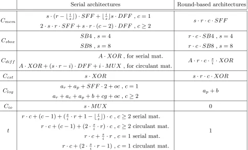
We now present the formulas for the estimates for the various parts of the ASIC implementations in Table1.
6.3 Discussion
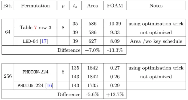
Table2 compares FOAM of some real implementations of LEDand PHOTONwith our estimated FOAM. Please note that the authors of [17] and [16] did not use the special optimization trick, described above. To reflect this, we provide two FOAMs, one taking the optimization into account and one which does not. ForLED[17] reports 966 GE forLED-64, where 299 GE are required to store the key state and around 40 GE are required for the key addition, multiplexers, and control logic. We thus compare with 627 GE. [20] reports 2,400 GE forAES-128 out of which 835 GE are required for the key schedule, thus we compare our FOAM to 1,565 GE. The authors chose a different optimization point, as can be seen in the higher area and significantly lower cycle count. We used the formulas above with the parameters ofPHOTON-224 (r = 8, c = 8, i = 4, s = 4, p = 8, serialized MDS) for the estimation of the 256-bit permutation. As PHOTONis, contrary to LED, an unkeyed permutation, the last row of Table2 is actually the best suited comparison. In summary, Table2underlines how close FOAM is to real implementations.
Please note that this is an upper bound for serial matrices, asZ may have coefficients that require less XORs thanr
times (Z0, . . . , Zr−1). At the same time is the critical path of the serial matrix aroundrtimes longer than the one for a circulant matrix.
Table 1: ASIC implementations estimation for the intermediate state memory cost Cmem, the S-boxes
implementation cost Csbox, the diffusion matrix implementation cost Cdif f, the constant addition Ccst,
the control logic costClog, the IO logic costCio and the numbertof clock cycles to perform one round.
Serial architectures Round-based architectures
Cmem s·(r− b
i
sc)·SF F +b
i
scs·DF F , c= 1
2·s·r·SF F +s·r·(c−2)·DF F , c≥2
s·r·c·SF F
Csbox SB4, s = 4
SB8, s = 8
r·c·SB4, s= 4
r·c·SB8, s= 8
Cdif f A·XOR , for serial mat.
A·XOR+ (s·r−i)·DF F +i·M U X , for circulant mat.
A·r·c· s
i ·XOR
Ccst s·XOR s·r·c·XOR
Clog ar+ap+SF F ·2 +oc , c= 1
ar+ac+ap+b+cg+oc , c≥2
ap+b
Cio s·M U X 0
t
r·c+ (c−1) + (si ·r+ 1− bi
sc)·c , c ≥2 serial mat.
r·c+ (c−1) + (2· s
i ·r)·c , c ≥2 circulant mat.
r·c+ si ·r , c = 1 serial mat.
r·c+ (2· s
i ·r−1) , c= 1 circulant mat.
1
7 Results and new diffusion matrices
In this section we provide the results of our framework, as well as new diffusion matrices that are very interesting for hardware implementations. As explained in Section 4, the designer’s input is the permutation bitsize n, the metric he would like to maximize (area or FOAM), and the degree up to which serial or round-based implementations are important. To illustrate our method, we focused on the case where the designer would like to build a 64-bit permutation (which is a typical state size for a lightweight block cipher). For the implementation types, we focused on three scenarios: only serial implementation is important, only round-based implementation is important, serial and round-based implementations are equally important for the designer.
Before describing our results, we first explain how we found good diffusion matrices (circulant and serial) and then list these matrices in the next three subsections. Our optimal matrices outperform known ones from theAES,LEDciphers and thePHOTONhash function.
7.1 Lightweight coefficients
Consider the AES matrix, a circulant matrix with coefficients (0x01, 0x01, 0x02, 0x03) over GF(28) defined by the irreducible polynomialα8+α4+α3+α+ 1. The matrix appears to be very lightweight due to the low Hamming weight of its entries. But surprisingly, we found an even lighter circulant matrix over the same field with coefficients (0x01,0x01,0x04,0x8d). We now explain why this is so.
We first illustrate how to compute the number of XORs required to implement a multiplication by a finite field element x. To do so, we use GF(28) defined by α8 +α4+α3 +α+ 1 as an example. Let
x=x7·α7+x6·α6+· · ·x1·α+x0 = (x7, x6,· · ·, x1, x0). Further, for ease of explanation, we employ
hexadecimal encoding: (x7, x6, x5, x4, x3, x2, x1, x0) can be encoded as a tuple of hexadecimal numbers
Table 2: Comparison of estimated FOAM with real implementations.
Bits Permutation p ts Area FOAM Notes
64 Table7row 3 8
35 586 10.39 using optimization trick
39 586 9.33 not optimized
LED-64 [17] 39 627 8.09 Area /wo key schedule
Difference +7.0% -13.3%
256 PHOTON-224 8
135 1842 0.27 using optimization trick
143 1842 0.26 not optimized
PHOTON-224 [16] 143 1735 0.29 Difference -5.6% +12.7%
(0x80, 0x40, 0x20, 0x10, 0x08, 0x04, 0x02, 0x01). Then, the multiplication of 0x04 and 0x08 by x can be represented respectively as:
0x04·x=(x5, x4, x3+x7, x2+x6+x7, x1+x6, x0+x7, x6+x7, x6)
=(0x20, 0x10, 0x88, 0xc4, 0x42, 0x81, 0xc0, 0x40),
0x08·x=(x4, x3+x7, x2+x6+x7, x1+x5+x6, x0+x5+x7, x6+x7, x5+x6, x5)
=(0x10, 0x88, 0xc4, 0x62, 0xa1, 0xc0, 0x60, 0x20).
It can be seen that the number of XORs required for the multiplication of 0x04 and 0x08 byx is 6 and 9 respectively. Now we can compute
0x8d·x= (α7+α3+α2+ 1)·x
= (0xb1, 0x58, 0x2c, 0x96, 0xfa, 0x4c, 0xa6, 0x62)
⊕(0x10, 0x88, 0xc4, 0x62, 0xa1, 0xc0, 0x60, 0x20)
⊕(0x20, 0x10, 0x88, 0xc4, 0x42, 0x81, 0xc0, 0x40)
⊕(0x80, 0x40, 0x20, 0x10, 0x08, 0x04, 0x02, 0x01) = (0x01, 0x80, 0x40, 0x20, 0x11, 0x09, 0x04, 0x03) = (x0, x7, x6, x5, x0+x4, x0+x3, x2, x0+x1)
Due to the ’cancellation of XORs’, we see that multiplication of x by 0x8d requires only 3 XORs. Similarly, the multiplication ofx by 0x02 and 0x03 requires 3 and 11 XORs respectively.
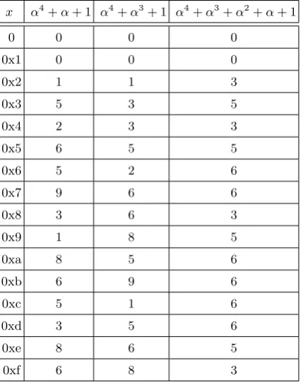
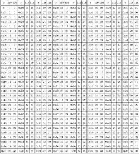
In a similar fashion, for the purpose of finding lightweight diffusion matrices, we compute the XOR count for each field element. Table 3 and Table 4 shows the XOR count for every element of the finite fieldsGF(24) andGF(28) defined by different irreducible polynomials, respectively.
Now we explain how to use the tables to calculate the number of XORs required to implement a row of a matrix, as denoted byAin Section6. Denote a given row of an r×r matrix by (x1, x2,· · ·xr) over
a finite field GF(2i). Let γ
j be the XOR count in Table 3 and Table 4 (i = 4 and i= 8 respectively)
corresponding to the field elementxj. ThenAis equal to (γ1+· · ·+γr)+(z−1)·i, wherezis the number of
non-zero elements in the row. We give some examples: row (0x1,0x1,0x4,0x9) uses (0 + 0 + 2 + 1) + 3×4 = 15 XORs to implement over GF(24); the AES matrix with coefficients (0x01,0x01,0x02,0x03) uses (0 + 0 + 3 + 11) + 3×8 = 38 XORs to implement per row over GF(28); the circulant matrix with coefficients (0x01,0x01,0x04,0x8d) uses (0 + 0 + 6 + 3) + 3×8 = 33 XORs to implement per row over
GF(28). This explains why the circulant matrix with coefficients (0x01,0x01,0x04,0x8d) is lighter than theAESmatrix.
Table 3: XORs required to implement a multiplication by x over GF(24) using different irreducible polynomials.
x α4+α+ 1 α4+α3+ 1 α4+α3+α2+α+ 1
0 0 0 0
0x1 0 0 0
0x2 1 1 3
0x3 5 3 5
0x4 2 3 3
0x5 6 5 5
0x6 5 2 6
0x7 9 6 6
0x8 3 6 3
0x9 1 8 5
0xa 8 5 6
0xb 6 9 6
0xc 5 1 6
0xd 3 5 6
0xe 8 6 5
0xf 6 8 3
7.2 Subfield construction
In this section, we describe the subfield construction which allows us to outperform the AES matrix even more than the optimal matrix found in Section7.1. As computed in the previous subsection, the MDS circulant matrixcirc(0x1,0x1,0x4,0x9) over GF(24) defined by α4+α+ 1 requires 15 XORs to implement per row. Using the method of [13, Section 3.3], we can form a circulant MDS matrix over
GF(28) by using two parallel copies ofQ=circ(0x1,0x1,0x4,0x9) over GF(24). The matrix is formed by writing each byteqj as a concatenation of two nibblesqj = (qjL||qjR). Then the MDS multiplication is
computed on each half (uL
1, uL2, uL3, uL4) = Q·(q1L, qL2, q3L, qL4) and (uR1, uR2, uR3, uR4) = Q·(q1R, q2R, q3R, q4R)
overGF(24). The result is concatenated to form four output bytes (u1, u2, u3, u4) whereuj = (uLj||uRj).
This matrix needs just 15×2 = 30 XORs to implement per row. In comparison, the lightest MDS circulant matrixcirc(0x01,0x01,0x04,0x8d) overGF(28) defined byα8+α4+α3+α+ 1 requires more
XORs (33 XORs per row).
Further, we can serialize the above multiplication to do the left half followed by the right half, in which case only 15 XORs are needed to implement one row of the MDS matrix over GF(28). Another
advantage of subfield construction is exemplified by theSPN-Hashconstruction [13]. It is difficult to find an 8×8 serial MDS matrix over GF(28) exhaustively. Instead, two parallel copies of the PHOTON 8×8 serial MDS matrix overGF(24) were concatenated to form the 8×8 serial MDS matrix overGF(28) for SPN-Hash.
It is straightforward to generalize this method to form a diffusion matrix with branch numberB over
GF(2s) from s/i copies of a diffusion matrix of the same branch number over a subfield GF(2i), where
idividess.
7.3 Good matrices
In this section, we list optimal low-weight circulant and serial matrices of different branch number over the finite fieldsGF(2), GF(22),GF(24) andGF(28). Using the construction of Section7.2, we can form diffusion matrices to transform nibbles and bytes from these subfields.
The optimal matrices are found by exhaustively checking the branch number of all matrices and choosing the one with the least number of XORs according to the method explained in Section 7.1. To
Table 4: XORs required to implement a multiplication by x over GF(28) using different irreducible polynomials.11b and 11d denoteα8+α4+α3+α+ 1 and α8+α4+α3+α2+ 1 respectively
x 11b 11d x 11b 11d x 11b 11d x 11b 11d x 11b 11d x 11b 11d x 11b 11d x 11b 11d
check the branch number of matrixQ, we concatenate it with the identity matrix Ir to form (Ir|Q), the
generating matrix of the corresponding linear code, and use the MAGMA software to find the distance. When we say a matrix has branch numberB, we mean the matrix has both differential and linear branch number equal toB. That is, we check that bothQand its transposeQt has branch number B.
We are aware that better techniques than naive exhaustive search might be used here. However, such improvements are not the goal of this article and we leave them as potential future work.
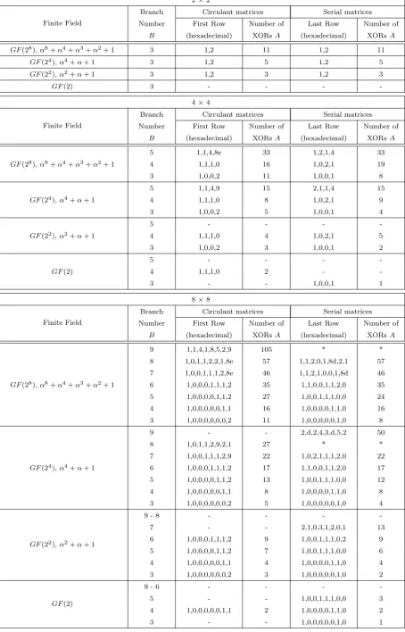
Circulant matrices. In Table 5, we list optimal r×r circulant matrices with branch numbers 3 to
r+ 1. The “First Row” column represents the first row of the circulant matrix (as described in Section 4). The “Number of XORs” column represents the number of XOR gates needed to implement one row of the circulant matrix.
The matrices are optimal in the sense that they need minimal number of XORs to implement. In the events of a tie between two matrices, possibly over different finite field representations, we just list one of them. For example, the circulant matrices circ(0x01,0x01,0x04,0x8d) over GF(28) defined by
α8+α4+α3+α+ 1 andcirc(0x01,0x01,0x04,0x8e) overGF(28) defined byα8+α4+α3+α2+ 1 both outperforms theAESmatrix by using 33 XORs to implement one row, so we just list the latter. We use “-” to represent that no circulant matrix with branch number B exists (verified either by exhaustive search or by coding theory bounds). For example, it can be verified that 8 × 8 circulant MDS matrix does not exist in the finite fieldGF(24).
The only exception where we did not find the optimal matrix is for 8×8 circulant MDS matrix over
GF(28). Because the search space is too big to exhaust, we just list theWHIRLPOOL matrix which is MDS and low weight.
Serial matrices. Here, in a similar fashion to the case of circulant matrices, we provide optimal low-weight serial matrices of various branch numbers over different finite fields.
In Tables 5, we list optimal r×r serial matrices with branch numbers 3 tor+ 1. The “Last Row” column represents the last row of the serial matrix (as described in Section4). The “Number of XORs” column represents the number of XOR gates needed to implement the last row. Again, we simply list one matrix in the event of a tie, and use “-” to represent that no serial matrix with branch numberB
exists. In addition, we use “*” to denote that we have not found the serial matrix with branch number
B at this point of time due to the huge search space. For instance, as the search space is too big to exhaust, we could not find a 8 × 8 serial MDS matrix over GF(28). In this case, we can employ the
method of subfield construction (described in Section7.2), i.e. use two parallel copies of the 8 ×8 MDS serial matrix with last row (0x2,0xd,0x2,0x4,0x3,0xd,0x5,0x2) (refer to second row of 8×8 subtable of Table5) over GF(24) to obtain the desired 8×8 serial MDS matrix over GF(28).
Note that the special structure of the serial matrices leads to the fact that only XORs for the last row are required. In particular, for anr×r serial matrix, we just need to implement the last row as an LFSR feedback function and iterate itr times to obtain the required matrix multiplication. This tactic has been adopted in [16,17] to define the PHOTONand LEDMDS matrices over GF(24) respectively. The last rows of the serial matrices are (0x2,0x4,0x2,0xb,0x2,0x8,0x5,0x6) and (0x4,0x1,0x2,0x2) respectively, which require 53 and 16 XORs to implement per row. In fact, we have found lighter serial matrices over the same finite field: 8 × 8 serial matrix with last row (0x2,0xd,0x2,0x4,0x3,0xd,0x5,0x2) requiring 50 XORs; and 4 ×4 serial matrix with last row (0x2,0x1,0x1,0x4) requiring 15 XORs (refer to 4×4 and 8×8 subtables of Table5).
7.4 Application: FOAM Comparison for 64-bit SPN Structures
Table 5: Good circulant and serial matrices of Size 2 ×2, 4 ×4 and 8×8
2×2
Finite Field
Branch Circulant matrices Serial matrices
Number First Row Number of Last Row Number of
B (hexadecimal) XORsA (hexadecimal) XORsA
GF(28),α8+α4+α3+α2+ 1 3 1,2 11 1,2 11
GF(24),α4+α+ 1 3 1,2 5 1,2 5
GF(22),α2+α+ 1 3 1,2 3 1,2 3
GF(2) 3 - - -
-4×4
Finite Field
Branch Circulant matrices Serial matrices
Number First Row Number of Last Row Number of
B (hexadecimal) XORsA (hexadecimal) XORsA
5 1,1,4,8e 33 1,2,1,4 33
GF(28),α8+α4+α3+α2+ 1 4 1,1,1,0 16 1,0,2,1 19
3 1,0,0,2 11 1,0,0,1 8
5 1,1,4,9 15 2,1,1,4 15
GF(24),α4+α+ 1 4 1,1,1,0 8 1,0,2,1 9
3 1,0,0,2 5 1,0,0,1 4
5 - - -
-GF(22),α2+α+ 1 4 1,1,1,0 4 1,0,2,1 5
3 1,0,0,2 3 1,0,0,1 2
5 - - -
-GF(2) 4 1,1,1,0 2 -
-3 - - 1,0,0,1 1
8×8
Finite Field
Branch Circulant matrices Serial matrices
Number First Row Number of Last Row Number of
B (hexadecimal) XORsA (hexadecimal) XORsA
9 1,1,4,1,8,5,2,9 105 * *
8 1,0,1,1,2,2,1,8e 57 1,1,2,0,1,8d,2,1 57
7 1,0,0,1,1,1,2,8e 46 1,1,2,1,0,0,1,8d 46
GF(28),α8+α4+α3+α2+ 1 6 1,0,0,0,1,1,1,2 35 1,1,0,0,1,1,2,0 35
5 1,0,0,0,0,1,1,2 27 1,0,0,1,1,1,0,0 24
4 1,0,0,0,0,0,1,1 16 1,0,0,0,0,1,1,0 16
3 1,0,0,0,0,0,0,2 11 1,0,0,0,0,0,1,0 8
9 - - 2,d,2,4,3,d,5,2 50
8 1,0,1,1,2,9,2,1 27 * *
7 1,0,0,1,1,1,2,9 22 1,0,2,1,1,1,2,0 22
GF(24),α4+α+ 1 6 1,0,0,0,1,1,1,2 17 1,1,0,0,1,1,2,0 17
5 1,0,0,0,0,1,1,2 13 1,0,0,1,1,1,0,0 12
4 1,0,0,0,0,0,1,1 8 1,0,0,0,0,1,1,0 8
3 1,0,0,0,0,0,0,2 5 1,0,0,0,0,0,1,0 4
GF(22),α2+α+ 1
9 - 8 - - -
-7 - - 2,1,0,3,1,2,0,1 13
6 1,0,0,0,1,1,1,2 9 1,0,0,1,1,1,0,2 9
5 1,0,0,0,0,1,1,2 7 1,0,0,1,1,1,0,0 6
4 1,0,0,0,0,0,1,1 4 1,0,0,0,0,1,1,0 4
3 1,0,0,0,0,0,0,2 3 1,0,0,0,0,0,1,0 2
GF(2)
9 - 6 - - -
-5 - - 1,0,0,1,1,1,0,0 3
4 1,0,0,0,0,0,1,1 2 1,0,0,0,0,1,1,0 2
active S-boxes and 1-round bound which involves only 1 active S-box. We also write down t, the time to compute one round for serialized implementation (the time tfor round based implementation is the constant 1, so it is not presented).
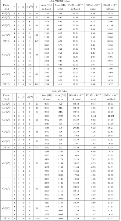
We compute the FOAM for round-based and serialized implementation based on the formula found in Section 6. We also present the FOAM for half-half implementation, where we take the average, i.e. equal weighting, of the round-based and serialized FOAM. This corresponds to implementations which are good for both scenarios. However, please note that this represents just one example, as the weighting of the scenarios is clearly a designer’s choice. The structure with the best area and FOAMs are presented in bold font.
We see that for designing 64-bit SPN:
1. For minimal area the geometry is the most important criterion, while the choice of the field of the MDS matrix is of less importance. The geometry should be chosen, such that c is maximized, and consequently, many internal columns can be realized with 1-input flip-flops. A serial matrix is favorable over a circulant matrix and in general smaller fields allow to save a few GE, but come at a high timing overhead.
2. When circulant matrices are used with PRESENT S-box in Table 6, the 4×4 almost-MDS circulant matrixcirc(0x1, 0x1, 0x1, 0x0) overGF(24) gives the best FOAM for round-based, serial and half-half implementations.
3. When circulant matrices are used with AES S-box in Table6, two parallel copies of the 4×4 MDS circulant matrix circ(0x1, 0x1, 0x4, 0x9) over GF(24) defined by α4+α+ 1 gives the best FOAM for round-based implementation. The 4×4 MDS circulant matrixcirc(0x01, 0x01, 0x04, 0x8e) over
GF(28) defined byα8+α4+α3+α2+1 gives the best FOAM for serial and half-half implementations. 4. When serial matrices are used with PRESENT S-box in Table 7, the 4×4 almost-MDS serial matrix with last row (0x1, 0x0, 0x2, 0x1) over GF(24) defined by α4 +α+ 1 gives the best FOAM for round-based, serial and half-half implementations.
5. When serial matrices are used withAESS-box in Table7, two parallel copies of the 4×4 MDS serial matrix with last row (0x2, 0x1, 0x1, 0x4) over GF(24) defined by α4+α+ 1 gives the best FOAM for round-based implementation. The 8×8 serial matrix (having branch number 6) with last row (0x01, 0x01, 0x00, 0x00, 0x01, 0x01, 0x02, 0x00) overGF(28) defined byα8+α4+α3+α+ 1 gives the best FOAM for serial and half-half implementations and is also very competitive for round-based FOAMs. It is thus a very interesting choice for many different applications.
6. Structures based onPRESENTS-box have higher FOAM for round-based and half-half implementations than those based onAESS-box. On the other hand, structures based onAESS-box have higher FOAM for serial implementation than PRESENTS-box, because they need significantly less rounds.
7. For structures using both types of S-boxes, 4×4 matrices have higher FOAM than 2×2 and 8×8 matrices.
8. Based on the above observations, we do not always go for the matrix with the best branch number: forPRESENTS-box in Tables 6and 7, we use almost-MDS 4×4 matrix which gives better trade-offs and a higher FOAM than MDS matrix. Moreover in Tables 6 and 7, when AES S-box is used with 8×8 matrices, we go for the one with branch number 6 instead of the optimal 9.
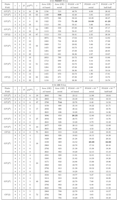
7.5 Designs with Optimal FOAM for Different Block Sizes
In Section 7.4, we showed a detailed comparison table for all possible configurations of 64-bit SPN structures based on AES and PRESENT S-box. From it, we extract the optimal design with the highest FOAM, which gives the best trade-off between speed, area and security.
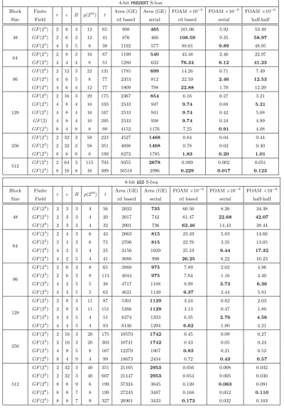
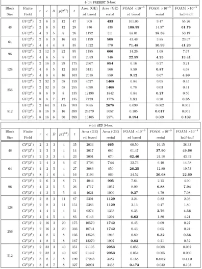
In this section, we apply the same computations to other common block sizes which are used in the construction of block ciphers and hash functions. The block sizes we consider are 48, 64, 96, 128, 256 and 512 bits. For conciseness and ease of reference, we only list the best FOAM values for each of these block sizes. In Table8, we list the designs with the best FOAM values based on circulant matrices. In Table9, we list the designs with the best FOAM values based on serial matrices.
Table 6: FOAM for 64-bit SPN based on circulant matrices and 4-bitPRESENT S-box or 8-bitAESS-box
4-bitPRESENTS-box
Finite
r c B p(264) t Area (GE) Area (GE) FOAM×10
−9
FOAM×10−9 FOAM×10−9
Field rd based serial rd based serial half-half
GF(24) 2 8 3 16 55 1156 541 46.76 3.88 25.32
GF(22) 2 8 3 16 87 1199 540 43.48 2.46 22.97
4 4 5 8 1579 652 50.16 5.77 27.96
GF(24) 4 4 4 8 51 1280 633 76.34 6.12 41.23
4 4 3 16 1156 630 46.76 3.09 24.92
GF(22) 4 4 4 8 83 1280 627 76.34 3.83 40.08
4 4 3 16 1199 629 43.48 1.90 22.69
GF(2) 4 4 4 8 147 1280 624 76.34 2.18 39.26
GF(24)
8 2 8 8
49
2091 873 28.58 3.35 15.96
8 2 7 10 1882 864 28.22 2.73 15.48
8 2 6 12 1669 851 29.92 2.35 16.14
8 2 5 14 1498 840 31.83 2.07 16.95
8 2 4 16 1284 827 37.89 1.87 19.88
8 2 3 22 1161 823 33.73 1.37 17.55
GF(22)
8 2 6 12
81
1712 834 28.45 1.48 14.96
8 2 5 14 1541 829 30.09 1.28 15.69
8 2 4 16 1284 821 37.89 1.15 19.52
8 2 3 22 1204 823 31.38 0.83 16.10
GF(2) 8 2 4 16 145 1284 818 37.89 0.64 19.27
8-bitAESS-box
Finite
r c B p(264) t Area (GE) Area (GE) FOAM×10
−9 FOAM×10−9 FOAM×10−9
Field rd based serial rd based serial half-half
GF(28) 2 4 3 6 27 2685 822 23.12 9.14 16.13
GF(24) 2 4 3 6 43 2663 815 23.49 5.83 14.66
GF(22) 2 4 3 6 75 2706 815 22.76 3.35 13.05
4 2 5 4 3150 1029 25.19 9.44 17.32
GF(28) 4 2 4 6 25 2792 988 21.39 6.82 14.10
4 2 3 8 2685 975 17.34 5.26 11.30
4 2 5 4 3086 990 26.25 6.22 16.23
GF(24) 4 2 4 6 41 2792 976 21.39 4.26 12.82
4 2 3 8 2663 968 17.62 3.25 10.44
GF(22) 4 2 4 6 73 2792 970 21.39 2.42 11.91
4 2 3 8 2706 968 17.07 1.83 9.45
GF(2) 4 2 4 6 137 2792 967 21.39 1.30 11.34
8 1 9 4 4688 1336 11.38 6.09 8.73
8 1 8 4 3663 1208 18.63 7.45 13.04
8 1 7 4 3428 1179 21.28 7.82 14.55
GF(28) 8 1 6 4 23 3193 1149 24.52 8.23 16.38
8 1 5 5 3027 1133 21.83 6.78 14.31
8 1 4 6 2792 1103 21.39 5.95 13.67
8 1 3 8 2685 1090 17.34 4.58 10.96
GF(24)
8 1 8 4
39
3599 1148 19.30 4.86 12.08
8 1 7 4 3385 1135 21.82 4.98 13.40
8 1 6 4 3171 1121 24.86 5.10 14.98
8 1 5 5 3005 1115 22.14 4.12 13.13
8 1 4 6 2792 1102 21.39 3.52 12.45
8 1 3 8 2663 1094 17.62 2.68 10.15
GF(22)
8 1 6 4
71
3214 1105 24.20 2.89 13.54
8 1 5 5 3048 1104 21.53 2.31 11.92
8 1 4 6 2792 1096 21.39 1.95 11.67
8 1 3 8 2706 1093 17.07 1.47 9.27
Table 7: FOAM for 64-bit SPN based on serial matrices and 4-bitPRESENT S-box or 8-bitAESS-box
4-bitPRESENTS-box
Finite
r c B p(264) t Area (GE) Area (GE) FOAM×10
−9 FOAM×10−9 FOAM×10−9
Field rd based serial rd based serial half-half
GF(24) 2 8 3 16 39 1156 513 46.76 6.09 26.42
GF(22) 2 8 3 16 63 1199 508 43.48 3.85 23.67
4 4 5 8 1579 586 50.16 10.39 30.27
GF(24) 4 4 4 8 35 1322 570 71.48 10.99 41.23
4 4 3 16 1113 561 50.41 5.66 28.04
GF(22) 4 4 4 8 55 1365 559 67.08 7.26 37.17
4 4 3 16 1113 556 50.41 3.67 27.04
GF(2) 4 4 3 16 87 1113 553 50.41 2.35 26.38
GF(24)
8 2 9 6
33
3074 794 17.64 8.01 12.82
8 2 7 10 1882 724 28.22 5.78 17.00
8 2 6 12 1669 711 29.92 5.00 17.46
8 2 5 14 1455 697 33.73 4.45 19.09
8 2 4 16 1284 687 37.89 4.02 20.95
8 2 3 22 1118 681 36.36 2.97 19.67
8 2 7 10 2053 700 23.72 4.00 13.86
8 2 6 12 1712 689 28.45 3.44 15.94
GF(22) 8 2 5 14 51 1455 681 33.73 3.02 18.37
8 2 4 16 1284 676 37.89 2.68 20.29
8 2 3 22 1118 675 36.36 1.95 19.16
8 2 5 14 1455 673 33.73 1.90 17.81
GF(2) 8 2 4 16 83 1284 671 37.89 1.67 19.78
8 2 3 22 1118 673 36.36 1.21 18.78
8-bitAESS-box Finite
r c B p(264) t Area (GE) Area (GE) FOAM×10
−9 FOAM×10−9 FOAM×10−9
Field rd based serial rd based serial half-half
GF(28) 2 4 3 6 19 2685 766 23.12 14.96 19.04
GF(24) 2 4 3 6 31 2663 750 23.49 9.56 16.53
GF(22) 2 4 3 6 47 2706 744 22.76 6.40 14.58
4 2 5 4 3150 898 25.19 18.22 21.71
GF(28) 4 2 4 6 17 2856 866 20.44 13.08 16.76
4 2 3 8 2621 836 18.20 10.51 14.36
4 2 5 4 3086 850 26.25 12.80 19.53
GF(24) 4 2 4 6 27 2834 839 20.75 8.77 14.76
4 2 3 8 2621 826 18.20 6.79 12.49
GF(22) 4 2 4 6 43 2877 828 20.13 5.65 12.89
4 2 3 8 2621 820 18.20 4.32 11.26
GF(2) 4 2 3 8 75 2621 818 18.20 2.49 10.35
GF(28)
8 1 8 4
16
3663 928 18.63 18.15 18.39 8 1 7 4 3428 899 21.28 19.35 20.32 8 1 6 4 3193 869 24.52 20.68 22.60 8 1 5 5 2963 844 22.79 17.53 20.16 8 1 4 6 2792 823 21.39 15.38 18.38 8 1 3 8 2621 802 18.20 12.15 15.18
GF(24)
8 1 9 4
24
4581 920 11.91 12.31 12.11 8 1 7 4 3385 845 21.82 14.59 18.20 8 1 6 4 3171 832 24.86 15.06 19.96 8 1 5 5 2963 823 22.79 12.30 17.54 8 1 4 6 2792 812 21.39 10.52 15.95
8 1 3 8 2621 802 18.20 8.10 13.15
8 1 7 4 3556 821 19.77 9.27 14.52
8 1 6 4 3214 810 24.20 9.52 16.86
GF(22) 8 1 5 5 40 2963 807 22.79 7.68 15.23
8 1 4 6 2792 802 21.39 6.48 13.93
8 1 3 8 2621 796 18.20 4.93 11.56
8 1 5 5 2963 799 22.79 4.35 13.57
GF(2) 8 1 4 6 72 2792 796 21.39 3.65 12.52
Table 8: FOAM for different block sizes based on circulant matrices and 4-bit PRESENT S-box or 8-bit AESS-box
4-bitPRESENTS-box
Block Finite
r c B p(264) t Area (GE) Area (GE) FOAM×10
−9 FOAM×10−9 FOAM×10−9
Size Field rd based serial rd based serial half-half
GF(22) 2 6 3 12 65 908 465 101.06 5.92 53.49
48 GF(24) 2 6 3 12 41 876 466 108.59 9.35 58.97
GF(24) 4 3 5 8 38 1192 577 88.01 9.89 48.95
64 GF(2
2) 2 8 3 16 87 1199 540 43.48 2.46 22.97
GF(24) 4 4 4 8 51 1280 633 76.34 6.12 41.23
GF(22) 2 12 3 22 131 1785 699 14.26 0.71 7.49
96 GF(24) 4 6 5 8 77 2353 812 22.59 2.46 12.53
GF(24) 4 6 4 12 77 1909 798 22.88 1.70 12.29
GF(22) 2 16 3 29 175 2367 854 6.16 0.27 3.21
GF(24) 4 8 4 16 103 2533 947 9.74 0.68 5.21
128 GF(22) 4 8 4 16 167 2533 941 9.74 0.42 5.08
GF(2) 4 8 4 16 295 2533 938 9.74 0.24 4.99
GF(24) 8 4 8 8 99 4152 1176 7.25 0.91 4.08
GF(24) 2 32 3 58 223 4527 1468 0.84 0.04 0.44
256 GF(22) 2 32 3 58 351 4698 1468 0.78 0.02 0.40
GF(24) 8 8 8 8 199 8272 1785 1.83 0.20 1.01
512 GF(2
2) 2 64 3 115 703 9355 2678 0.099 0.002 0.051
GF(24) 8 16 8 16 399 16518 2996 0.229 0.017 0.123
8-bitAESS-box
Block Finite
r c B p(264) t Area (GE) Area (GE) FOAM×10
−9 FOAM×10−9 FOAM×10−9
Size Field rd based serial rd based serial half-half
GF(22) 2 3 3 4 56 2033 735 60.50 8.26 34.38
48 GF(24) 2 3 3 4 20 2017 742 61.47 22.68 42.07
GF(28) 2 3 3 4 32 2001 736 62.46 14.43 38.44
GF(24) 2 4 3 6 43 2663 815 23.49 5.83 14.66
64 GF(2
2) 2 4 3 6 75 2706 815 22.76 3.35 13.05
GF(28) 4 2 5 4 25 3150 1029 25.19 9.44 17.32
GF(24) 4 2 5 4 41 3086 990 26.25 6.22 16.23
GF(24) 2 6 3 8 65 3980 975 7.89 2.02 4.96
96 GF(2
2) 2 6 3 8 113 4044 975 7.64 1.16 4.40
GF(28) 4 3 5 5 38 4717 1188 8.99 3.73 6.36
GF(24) 4 3 5 5 62 4621 1149 9.37 2.44 5.91
GF(24) 2 8 3 11 87 5301 1129 3.24 0.82 2.03
128 GF(2
2) 2 8 3 11 151 5386 1129 3.13 0.47 1.80
GF(28) 4 4 5 4 51 6274 1333 6.35 2.76 4.56
GF(24) 4 4 5 4 83 6146 1294 6.62 1.80 4.21
GF(24) 2 16 3 20 175 10570 1742 0.45 0.09 0.27
256 GF(2
2) 2 16 3 20 303 10741 1742 0.43 0.05 0.24
GF(24) 4 8 5 8 167 12270 1907 0.83 0.21 0.52
GF(28) 8 4 9 4 99 18673 2434 0.72 0.43 0.57
GF(24) 2 32 3 40 351 21105 2953 0.056 0.008 0.032
GF(22) 2 32 3 40 607 21447 2953 0.054 0.005 0.030
512 GF(28) 8 8 9 6 199 37324 3645 0.120 0.063 0.091
GF(28) 8 8 7 8 199 27243 3487 0.168 0.052 0.110