1/20
“Memory of Water” Experiments Explained with No Role Assigned to Water:
Pattern Expectation after Classical Conditioning of the Experimenter
Francis Beauvais 1, *
1 Scientific and Medical Writing, 91 Grande Rue, 92310 Sèvres, France * Correspondence: [email protected]; Tel.: +33 6 68 36 58 36
ABSTRACT
The “memory of water” experiments suggested the existence of molecular-like effects without molecules. Although no convincing evidence of modifications of water – specific of biologically-active molecules – has been reported up to now, consistent changes of biological systems were nevertheless recorded. We propose an alternate explanation based on classical conditioning of the experimenter.
Using a probabilistic model, we describe not only the biological system, but also the experimenter engaged in an elementary dose-response experiment. We assume that during conventional experiments involving genuine biologically-active molecules, the experimenter is involuntarily conditioned to expect a pattern, namely a relationship between descriptions (or “labels”) of experimental conditions and corresponding biological system states.
The model predicts that the conditioned experimenter could continue to record the learned pattern even in the absence of the initial cause, namely the biologically-active molecules. The phenomenon is self-sustained because the observation of the expected pattern reinforces the initial conditioning. A necessary requirement is the use of a system submitted to random fluctuations with autocorrelated successive states (no forced return to the initial position). The relationship recorded by the conditioned experimenter is, however, not causal in this model because blind experiments with an “outside” supervisor lead to a loss of correlations (i.e., system states randomly associated to “labels”).
In conclusion, this psychophysical model allows explaining the results of “memory of water” experiments without referring to water or another local cause. It could be extended to other scientific fields in biology, medicine and psychology when suspecting an experimenter effect.
Keywords: Experimenter effect; “Memory of water”; Classical conditioning.
1. Introduction
The violence of the controversy had most probably its roots in the “two centuries of observation and rationalization” that these results were supposed to reconsider.3 Because the idea that a “structuration” of water could mimic the effects of biologically-active molecules was considered impossible, the inevitable conclusion was that the experiments were flawed. As a consequence, there was no place for an alternate theoretical framework that would consider these results, without involving water and its alleged “memory”. The fact that this study could support homeopathy, also highly controversial, was another reason for this strong opposition. It is out of the scope of this article to describe this controversy; details on the debate and disputed experiments can be found elsewhere.1, 4, 5
According to the judgement of many scientists, there was nothing to explain in these experiments as there was no scientific facts, only poor science. Therefore, the report of Nature’s investigation in Benveniste’s laboratory has been generally considered to put the last word to the public debate.6, 7 Nevertheless, some authors reported modifications of physical parameters of highly-diluted solutions or proposed different theoretical frameworks.8-13 How the specificity of the initial molecule could be conveyed through the successive dilutions remained however unanswered in these various theoretical frameworks. Moreover, correlations of changes of water parameters and corresponding changes of a biological model have not been described up to now.
My purpose in this introduction is not to fuel this debate again but simply to structure the arguments from both sides to explain why Benveniste failed to convince his peers. Indeed, after the basophil model described in 1988 in Nature’s article, other experimental models, mainly isolated rodent heart and plasma coagulation, were developed by Benveniste’s team. Experimental data accumulated seemingly in favor of a role of water for storing information on molecules in solution.14-20 During this period, Benveniste made a step further by stating that molecular information could be “imprinted” in water through electromagnetic fields (1992) as in a magnetic tape 15 and could be even digitized (1995).20 At this occasion, he coined the expression “digital biology”.20, 21
In Table 1, arguments from Benveniste’s experiments in favor of or against “memory of water” are summarized. The arguments in favor of “memory of water” are mainly the observation of “activated” states of the biological systems associated to test samples “imprinted” with different methods and the apparent specificity of the biological effects. The arguments against “memory of water” are mostly difficulties to reproduce the results by other teams and the absence of a compelling theoretical framework. There is also another reason – less known – that prevented Benveniste to go further in his quest of the perfect experiment that would be totally convincing. This reason was a stumbling block that was more particularly highlighted during public demonstrations where colleagues from other teams were invited to supervise proof-of-concept experiments. The role of these outside supervisors was to produce “inactive” and “active” test samples (water samples with high dilutions or “imprinted” water; computer files for digital biology) and to mask them under a code number. After the outside supervisors had left, the coded samples were tested by Benveniste’s team. When all measurements were completed, the results were sent to the supervisors who assessed the rate of success by comparing for each run the measured system state and the corresponding “label” (unbeknown of the experimenter who did the test). These proof-of-concept experiments systematically failed in the sense that “activated” states were always randomly distributed between test samples with “inactive” and “active” labels.1, 22, 23
In this article, I propose to simultaneously take into consideration Benveniste’s experiments and to abandon the “memory of water” hypothesis. A theoretical framework is constructed where these experiments are related to an experimenter effect, which is the consequence of a previous classical conditioning of the experimenter. In this setting, all test samples are nothing more than controls (or placebos) and the different procedures to “imprint” water samples are nothing more than rituals. The proposed model describes all features of Benveniste’s experiments: emergence of an “activated state” of a biological system without local cause, correlations between “labels” and system states, and mismatches of outcomes in blind experiments with an outside supervisor. No role is attributed to water or another local cause but now the attention shifts to the experimenter. The proposed experimenter effect is original and could have consequences beyond the “memory of water” controversy. Therefore, considering Benveniste’s experiments only as an example of specious science misses the point and prevents from seeing what these experiments could teach us. The price that the proponents of “memory of water” have to pay is abandoning the initial hypothesis (i.e., a molecular-like effect without molecules). For the opponents, the price to pay is to accept that these weird experiments – admittedly misinterpreted by their authors – had nevertheless a scientific interest.
Table 1. The arguments for and against molecular-like effects without molecules in Benveniste’s experiments.
Arguments for Arguments against
•Emergence of an “activated” state of biological
models mimicking the effect of biologically-active molecules a
• Emergence of a relationship between experimental conditions and states of system
• Specificity of the molecular-like effects b
• Consistency of the results with different
experimenters, biological systems and procedures
• Successful tests in blind experiments with local/inside supervisor or automated devices. c
• Not compatible with current scientific knowledge on water (e.g., very short half-lives of chemical bonds between water molecules)
• Not compatible with current scientific knowledge on biochemical interactions (e.g., law of mass action)
• No compelling theoretical framework
• Difficulties to reproduce the results by other teams
• Proximity with homeopathy
• Loss of correlations in blind experiments with an outside supervisor. c
a In “memory of water” experiments, water samples are supposed to induce a biological activity although
the biologically-active molecules have been removed via extensive serial dilutions (“high dilutions”) or after water samples have been “imprinted” through electromagnetic fields using different devices (“electronic transmission” or “digital biology”).
b Water samples supposed to have been “imprinted” apparently retained the specificity exhibited by the
original molecules (“imprints” of biologically-inactive molecules were inactive even if their structure was close to biologically-active molecules).
c See definitions of “inside” or “outside” supervisors in section “Consequences of blind experiments on
correlations”.
2. Classical conditioning during ordinary dose-response experiments
experimenter who handles an experimental system. Classical conditioning supposes first an “unconditioned stimulus” that produces an “unconditioned response” in an organism. In the well-known example of Pavlov’s dog, smelling or tasting food (unconditioned stimulus) induces salivation (unconditioned response). The purpose of the learning is to pair a “neutral stimulus” to the unconditioned stimulus. In this case, a bell (neutral stimulus) systematically rings just before food (unconditioned stimulus) is presented to the dog. Thus, the dog learns to associate the ring of the bell and the coming of food. During this learning process, the former neutral stimulus becomes a “conditioned stimulus”. Indeed, salivation (conditioned response) is now induced when the bell rings. To be complete, we must add that no food is expected (no salivation) by the dog when the bell does not ring. Thus, a relationship is established between the conditioned stimulus (ring vs. no ring) and the conditioned response (salivation vs. no salivation).
The purpose of most in vitro or physiology experiments is to study the effect of a biologically-active compound on a biological system. A dose-response is performed, meaning that the effect of the compound at different concentrations (0, x, 2x, 3x, etc.) is evaluated. For simplifying, we suppose that only one “active” condition versus one “inactive” condition (or control) is assessed during the experiments. We suppose also that the biological system has only two states: “resting” state (not different from background noise) and “activated” state (different from background noise).
In such experiments, one usually forgets that the biologically-active compound has not only a direct effect on the biological system but also an indirect effect on another “biological system”, namely the experimenter. Even with automated systems, there is always an experimenter who prepares the experiment, records the outcomes and interprets them. Therefore, it is easy to take a step further and to consider that during the repetitions of experiments, the experimenter unintentionally learns to combine the experimental conditions with the states of the biological system. Thus, the “inactive” condition (control) is associated to the “resting” state and the “active” condition (biologically-active molecules at pharmacological concentrations) is associated to the “activated” state.
After this classical conditioning process, the cognitive structures of the experimenter are changed. The“labels” of the experimental conditions are associated to the respective system states: “inactive” label is associated to “resting” state and “active” label is associated to “activated” state.
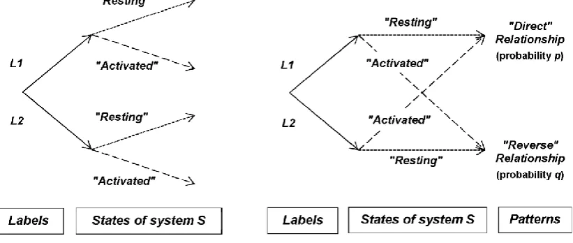
In the model that we construct, we posit that all samples to be tested are identical and are all biologically inactive in the sense that they do not induce a local causal biological effect. Even if the test samples are subjectively named “inactive” or “active” by the experimenter, it would be impossible to distinguish one test sample from another one on physical bases; only their identification with “labels” – in other words their meaning for the experimenter – is different. “Labels” are nothing more than a short description for the experimenter about the expected state of the experimental system.In Figure 1, the “labels” have the nonspecific names L1 or L2 that do not presuppose to which experimental condition (“inactive” or “active”) they are respectively associated by the experimenter.
It is important to underline that a relationship (direct or reverse) has a higher degree of abstraction than its components (“labels” and system states). A relationship is similar to a pattern (or a shape) that is thought in its wholeness, not as the simple sum of its individual components. In other words, after conditioning, the experimenter expects an “image” (a continuous entity), not “pixels” (discrete stuffs).
Figure 1. Expectation of patterns by the experimenter after classical conditioning. The two
“labels” (L1 vs. L2) and the two possible system states (“resting” vs. “activated”) define four couples of outcomes (A). The “labels” have the nonspecific names L1 or L2 which do not
presuppose to which of the two experimental conditions (“inactive” or “active”) they are
respectively associated by the experimenter. After classical conditioning (i.e., Pavlovian
conditioning) with “conventional” experiments involving biologically-active molecules at pharmacological concentrations, the two possible relationships expected by the experimenter are
named “direct” or “reverse” relationships with probabilities p and q, respectively (B). A relationship has a higher degree of abstraction than its components and is similar to a pattern that is thought in its wholeness, not as the simple sum of its individual components.
3. Consequences of the classical conditioning of the experimenter for future outcomes
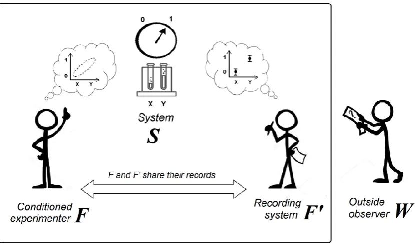
In this section, we explore the probabilistic consequences of the classical conditioning of an experimenter named F who records the state of the experimental system S (Figure 2). These probabilistic consequences are described in three sequential steps:
Figure 2. Description of the experimental situation.An elementary dose-response experiment is performed by an experimenter F who has been conditioned to expect a pattern. This pattern is the relationship between the descriptions X, Y (“labels”) of different experimental conditions and the
corresponding system states (0, 1). An observer F’ records the outcomes and, at the end of the experiment, F and F’ share their records.
Note that F’ does not need to be conditioned. Furthermore, F’ does not need to be human and can be replaced by any recording device. In this case, F takes note of the outcome of the experiment that has been recorded by F’ after the experiment is finished. The observer F’ is nothing more than an instance of the environment that keeps track of the outcomes.
Step 2: The outcome does not preexist. As the future outcome to be recorded by F is a property of F-S taken as a whole (not the simple addition of properties of F and S), it means that the outcome (direct or reverse relationship) is created when F and S join together to form F-S (i.e.,when F records the state of S). In other words, the outcome does not preexist its record by F.a A probability can nevertheless be attributed before the experiment to each possible future outcome (direct or reverse relationship) to be recorded by F.
Step 3: Independence of the future outcome. We have now to translate into mathematical terms an outcome that does not preexist its record.
We introduce an observer named F’ who records the state of F (correlated to the state of S). We describe the states of F, S and F’ from a point of view outside the laboratory (observer W). The interest of this outside point of view will appear later.b
The future outcome A to be recorded by F and the future outcome B to be recorded by F’ are independent events. Indeed, suppose that the outcomes A and B are perfectly correlated. If F’ is the first to record the outcome of the experiment (direct or reverse relationship), then the value of A
is fixed and preexists the interaction of F with S. Therefore, if we want to describe the outcome A
not preexisting its record by F, it must be independent from the outcome B.
By definition, the two events A and B are independent if their joint probability – i.e., the probability to be observed together – is the product of their respective probabilities:
Prob (AB) = Prob (A) × Prob (B) (Eq. 1)
4. Probability of a direct relationship with a conditioned experimenter
The different combinations of the future independent outcomes A and B to be recorded by F and F’
from a point of view outside the laboratory (observer W) are described in Figure 3.
Figure 3. Description of the possible future independent outcomes to be recorded by F and F’. The states of F, S and F’ are described from a point of view outside the laboratory. Each possible event to be recorded by the participants is composed of a label (L1 or L2) and a state of S, either
“resting” (↓) or “activated” (↑). These future events are independent but only some of them are shared by F and F’ (see Figure 4).
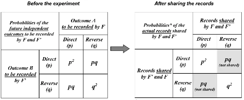
The probability for each observer to record a direct relationship is denoted p and the probability to record a reverse relationship is denoted q (with p + q = 1). Based on the independence of the future outcomes to be recorded by F and F’, Figure 4 can be built using Eq. 1. For a given participant, the probability p is the sum of p2 (probability that both F and F’ record “direct”) and pq (probability that this participant records “direct” and the other one records “reverse”).
Figure 4. Future outcomes to be recorded and shared records. The independence of the future outcomes to be recorded by the observers F and F’ has probabilistic consequences that are depicted in this figure. The left panel describes the probabilities of the possible future independent outcomes (direct or reverse relationship) to be recorded by the observers F and F’ before the experiment. The two events A and Bare independent (see section “Consequences of the classical conditioning of the experimenter for future outcomes”). The right panel describes the actual records shared by F and
F’. Example of records that are not shared: record of a “resting” state of S by F (direct relationship)
and record of an “activated” state of S by F’ (reverse relationship) for the same label L1.
After the experiment is completed, F and F’ share their records of all elementary outcomes (association of the “label” of each test sample with the corresponding system state). Only the records where F and F’agree on the concordance of their records are shared.c Therefore, situations with a probability equal to pq are not included in the list of the actual outcomes shared by F andF’
(Figure 4).
Note that F’ does not need to be human and can be any recording device. In this latter case, after the experiment is finished, F records each elementary outcome (outcome A with probability p) and the recording device F’ does the same for F-S (outcome B, independent from outcome A, with probability p). Then F takes note of the concordance of all recorded outcomes A and B (i.e., A = B
for each association of a “label” and the corresponding system state). The observer F’ is nothing more than an instance of the environment that keeps track of the outcomes.
Because the total probability of the outcomes shared by F and F’ must remain equal to one, a renormalization is necessary for probability calculation. For this purpose, the probability of each shared record is divided by the sum of the probabilities of all records possibly shared by F and F’
(Figure 4). The probability that F and F’ share a record of a direct relationship is:
2 2 2 ) ( Prob q p p direct +
= (Eq. 2)
We now write Eq. 2 to obtain only p as a variable by dividing both numerator and denominator by p2and by considering that q = 1 – p:
2 1 1 1 1 ) ( Prob − + = p direct (Eq. 3)
This equation can be generalized from 2 to N observers by supposing that the future outcomes to be observed by the N observers are independent (i.e., at least N – 1 observers are conditioned) and are shared by the N observers. In Eq. 2, the square exponents are replaced by N and we finally obtain: N p direct − + = 1 1 1 1 ) ( Prob (Eq. 4)
This generalized equation allows calculating the special case N = 0, which is the experimental situation in the absence of any observer:
2 1 1 1 1 1 1 1 1 0 0 = + = − + = p p (Eq. 5)
Starting from this situation without observer, we introduce again the observers F and F’ in the model by using Eq. 3 and by replacing p with p0 = 1/2. We obtain again Prob (direct) = 1/2. At first sight, the introduction of an experimenter – conditioned or not – in the model has no advantage over the classical approach. Indeed, considering that the outcome preexists to its record (classical approach) or does not preexist (present model) leads to the same result; direct and reverse relationship are evenly observed (only the “resting state” of S is observed). This is consistent with common sense: two control situations (or two placebos)are both associated to the “resting state”, regardless of the presence or not of an observer.
The advantage of the present model is seen in the next section after considering the fluctuations inherent to any measurement with a macroscopic system.
5. Emergence of correlations between “labels” and system states
Any macroscopic system is associated with random fluctuations. We note εn (with | εn | << 1) a small fluctuation of Prob (direct) at time tn.
We have seen that before the observation of the system, Prob (direct) = p0 = 1/2. At time t1, after the first fluctuation ε1, the new value of Prob (direct) is p1 that is calculated by replacing p0 with p0ε1 in Eq. 3. Note that a fluctuation of Prob (direct) different of zero means that the “activated” state of S can be possibly recorded by F even though with a tiny probability.
• In the first case where the system comes back to its initial position after each fluctuation, pn+1 is calculated with pn = p0 = 1/2:
1 1
n ( ) 1/2
Prob+ direct = n+
(with p0 = 1/2) (Eq. 6)
• In the second case, each state n is the starting point of the state n+1. A mathematical sequence is obtained where each pn is used for the calculation of pn+1:
2 1 n 1 n 1 n 1 1 1 1 ) ( Prob − + = = + + + n ε p p
direct (with p0 = 1/2)
(Eq. 7)
The distinction between return to initial position and new position as a starting point for the next state allows specifying systems that have different behaviors confronted with small random fluctuations. Thus, in Eq. 6, no specific relationship is established between “labels” and system states. Such systems can be qualified as “rigid” because small fluctuations do not move the system state away from the initial position. For example, internal thermal agitation induces small vibrations of a coin, but the inertia is sufficiently high that an immobile coin has practically no chance of jumping from head to tail within a reasonable timeframe. Similarly, after tossing, the trajectory of the coin can be considered as not influenced by internal thermal agitation. These systems that are “set to zero” after each tiny fluctuation have no interest for the present issue. Nevertheless, they allow underscoring that any experimental system submitted to random fluctuations is not necessarily suitable to observe significant correlations between “labels” and system states. In the second case described by Eq. 7, the experimental system may move away from its initial position due to random fluctuations (no forced return). Each new state is dependent on the previous one (autocorrelation). A classical example is a pollen grain on water surface. In this case, the grain is sufficiently small and with sufficient degrees of freedom to move away from its initial position because of the thermal agitation of water molecules. Biological systems are more complex but some of them have sufficient degrees of freedom to move from a “resting” state to an “activated” state after a series of random fluctuations (e.g., coronary dilatation of isolated rodent heart in Benveniste’s experiments). Biological system must be understood in an extended sense; thus, biochemical systems can also be suitable (e.g., in vitro coagulation with fibrinogen and thrombin in Benveniste’s experiments).
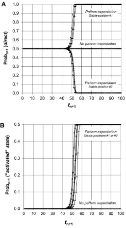
The mathematical sequence described by Eq. 7 is computed in Figure 5. After a series of tiny fluctuations, there is always a dramatic transition of Prob (direct) from 1/2 to 0 or 1, at random for each run. This transition reveals an instability of the initial situation (p0 = 1/2) after the introduction
Figure 5. Computer calculation of the model. The mathematical sequence of Eq. 7 was calculated and eight computer calculations are showed. Each probability fluctuation εn+1 during an elementary
time interval was randomly obtained in the interval from –0.5 × 10⁻¹⁵ to +0.5 × 10⁻¹⁵. Panel A
describes the probability of observing a direct relationship. There is a dramatic transition from 1/2 to 0 or 1 at random after a series of fluctuations due to the breaking of the initial symmetry. The tiny random fluctuations reveal the instability of the mathematical sequence for calculating Prob (direct). The consequence is the establishment of a relationship between “labels” (L1 vs. L2) and system states (resting state vs. activated state). The probability to observe an “activated” state increases from ε to 1/2; indeed, each test with “active” label is associated to an “activated” state (Panel B). In contrast, in the absence of conditioning, Prob (direct) is equal to 1/2 ± εn and there is no emergence of an
In a real experimental situation, before testing any sample (with “inactive” or “active” label), the system is prepared in a “resting” state (control condition) that is implicitly associated to the “inactive” label. In stable position #1, the label L1 is the “inactive” label and therefore the label L2 is the “active” label; conversely, in stable position #2, the labels L1 and L2 are the “active” and “inactive” labels, respectively.
Therefore, the mathematical sequence described in Eq. 7 allows explaining simultaneously two major features of Benveniste’s experiments, namely the emergence of an “activated” state from background noise and the significant correlations between “labels” and system states (Figure 5). No hypothesis on the physical properties of test samples or another local cause has been necessary.
Application to “memory of water” experiments. Perhaps the strongest argument in favor of a “memory” related to water was the emergence of an “activated” state of the biological system. This was particularly striking in Benveniste’s experiments with an isolated rodent heart that allowed “live” demonstrations of the coronary flow variations. Moreover, from 1992 to 1996, the experiments with the isolated rodent heart were performed using two systems that worked in parallel.1 These parallel experiments were used to confirm the measurement of each test sample, particularly in experiments designed as proof of concept. In a previous publication, I reanalyzed the duplicate outcomes of a series of experiments performed with this double system.22 These results were pooled regardless of the method used to “inform” water. The high correlation of the duplicate measurements (changes of coronary flow) was a very strong argument indicating that these experiments had an internal consistency and deserved to be considered through a scientific approach.
6. Consequences of blind experiments on correlations
In this section, we see how the model predicts the vanishing of the correlations between “labels” and system states in blind experiments with an outside supervisor.
We suppose that the observer W provides F with test samples under a coded name (the “inactive” and “active” labels are masked). When the experiments are ongoing, W is outside the laboratory and does not interact with F-S. After all states of S associated to the series of test samples have been recorded by F, these results are sent to W. The two lists, namely “labels” (unknown to F) and the states of the system recorded during the experiments, are compared by the supervisor W to assess the rates of direct/reverse relationships.
In this setting, there is a transfer of the information about labels from the inside to the outside: there is a loss of information for F-S and a gain for W. The experimenter F continues to expect a pattern, but no information is available on the label of each sample. Therefore, the “activated” state is evenly distributed among samples with “L1” and “L2” labels: Prob (directL2) = Prob (reverseL1) = 1/2;
consequently, Prob (direct) = Prob (reverse) = 1/2 (see Figure 1). This means that there is no relationship between “labels” and system states although the “activated” state is still observed (but associated indifferently to “L1” or “L2” labels). With an outside supervisor, the states of the entity F-S (direct and reverse relationships) are dissociated into their different components, namely labels on the one hand and states of S on the other hand. This experimental situation with an outside supervisor can be summarized as follows:
Prob (direct) = Prob (L1) × Prob (directL1) + Prob (L2) × Prob (directL2)
= 1/2 × 1/2 + 1/2 × 1/2 = 1/2 (Eq. 8)
Blind experiments can also be performed with a local/inside supervisor (F’ for example) or with an automatic device for the blind random choice of “labels”. In this setting, all participants and devices are inside the laboratory. From the point of view of W, the local supervisor or the automatic device is nothing more than a part of the system S and the outcome is a property of F-S taken as a whole as previously described for open-label experiments. In this situation, the emergence of a significant relationship between “labels” and system states is predicted as previously seen with Eq. 7:
Prob (direct) = 0 or Prob (direct) = 1 (Eq. 9)
Blind experiments with or without an outside supervisor have therefore different consequences on the experimental outcomes. These differences cannot be described within a classical framework that considers that in all cases the “whole” (pattern) is the simple sum of its parts (labels plus states of S).
Application to “memory of water” experiments. The vanishing of the apparent relationship in proof-of-concept demonstrations with an outside supervisor was a stumbling block for Benveniste’s experiments. This weird phenomenon could be considered as the scientific fact that emerges from Benveniste’s experiments. It is important to emphasize that despite the disappearance of correlations, activated states persisted – as described in this model – but they were randomly associated with “inactive” and “active” labels.1, 22 As explained in the introduction, the spreading of “activated” states regardless of “labels” was interpreted as the consequence of external disturbances. However, further improvements of experimental conditions and devices did not prevent this unwanted phenomenon.25, 26
of precautions had been taken and nevertheless the disturbing effect of an outside supervisor was clearly evidenced.
7. Experimenter’s conditioning as a stepwise learning process
For simplicity, we considered in a first approach that the classical conditioning of the experimenter was 100% efficient. However, as in every learning process, conditioning can be only partial. In this section, we complete the model for situations between no conditioning and perfect conditioning. These considerations also allow deepening the understanding of the probabilistic consequences of the conditioning of the experimenter.
In a first step, we vary the degree of independence of the future events A and B to be recorded by F and F’, respectively. We generalize Eq. 1 by adding a parameter named d:
Prob (AB) = Prob (A) × Prob (B) + d (with 0 ≤ d ≤ 1) (Eq. 10)
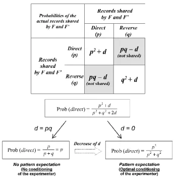
The future events A and B are independent if d = 0; their degree of correlation increases when d increases (d can be understood as the abbreviation of “dependence”). In a second step, the generalization of Eq. 3 follows (Figure 6):
d q p d p direct 2 ) (
Prob 2 2
2
+ +
+
= (with 0 ≤ d ≤ pq) (Eq. 11)
If d = 0, Eq. 11 is equal to Eq. 2 and after introduction of probability fluctuations there is a dramatic shift from 1/2 toward 1 or 0 as previously shown with Eq. 7. In contrast, the future events
A and B are perfectly correlated with d = pq and we find again the classical situation:
p q p p q p q p p pq q p pq p direct = + = + + = + + +
= 2 2 2 2
) ( ) ( 2 ) (
Prob (Eq. 12)
Probability fluctuations can be introduced in Eq. 12:
pn+1 = pn ± εn+1(with p0 = 1/2) (Eq. 13)
We easily see with Eq. 13 that there is no dramatic transition from p0 = 1/2 toward 0 or 1 and therefore no emergence of the “activated” state of S; there are only tiny fluctuations of Prob (direct) around 1/2. It is as if there was only one future event (A and B are perfectly correlated) that existed before its record. Therefore, varying the value of d from pq to 0 allows describing the progressive shift from no conditioning (no pattern expectation) to optimal experimenter’s conditioning (pattern expectation) (Figure 7). Even with a slight conditioning (value of d near 1/4), Prob (direct) is > 1/2. In this case, provided that the statistical power is sufficient, significant correlations between “labels” and system states could be evidenced.
Figure 6. Shift from no conditioning to conditioning of the experimenter. The conditioning process is more or less complete; this is mathematically translated by varying the degree of independence of the future outcomes to be observed by F and F’. The change of the parameter d from pq to 0 is
therefore an assessment of the experimenter’s conditioning to expect a pattern (a relationship). When
d = pq, the experimental outcome is a property of S alone (no conditioning) and, when d = 0, the experimental outcome is a property of F-S taken as whole (optimal conditioning of experimenter).
Figure 7. Experimenter’s conditioning as a stepwise learning process. The probabilities of Prob (direct) achieved with different value of d from 1/4 to 0 are calculated in panel A. The maximal value (stable position) achieved by Prob (direct) as a function of the value of d is depicted in panel B. In the absence of probability fluctuations (ε = 0) or if d = p0q0 = 1/4, Prob (direct) = 1/2, meaning,
that there is no relationship between “labels” and system states. Only with probability fluctuations
(± ε) and with values of d ≠ 0, correlations between “labels” and system states emerge as a function of d value. For simplicity, only data corresponding for L1 as “inactive” label are shown. For this figure, each probability fluctuation εn+1 during an elementary time interval was randomly obtained in
the interval from –0.5 × 10⁻⁵ to +0.5 × 10⁻⁵.
8. Discussion
Model and Benveniste’s experiments. The strong point of this model is that all features of Benveniste’s experiments are described: 1) emergence of an “activated state” from the background noise of a biological system without local cause; 2) correlations between “labels” and system states; 3) mismatches in outcomes from blind experiments with an outside supervisor. It is important to insist that these characteristics emerge from the formalism and are not ad hoc hypotheses. The model rests on reasonable assumptions about the measurement process of a biological experiment aimed to establish an elementary dose-response. Classical conditioning is also a plausible hypothesis. Moreover, the conditioning is self-sustained because the observation of the expected pattern reinforces it. Indeed, the more significant correlations are recorded by the experimenter, the more these correlations have a chance to be recorded in the next experiments.
This hypothetical model suggests that some cognitive processes (namely classical conditioning) might extend to systems spatially separated from the experimenter. It is important to underscore that there is no action at a distance, but coordination of events according to a structuring pattern. Thanks to their plasticity and degrees of freedom, biological systems appear the most suitable among the possible experimental models to evidence such non-classical relationships between observers and systems.
The model needs to be built from a point of view outside the laboratory. Indeed, from an “inside” point of view, the states of F, S and F’ are strictly correlated at any time. In contrast, only an outside point of view allows describing the independence of the future outcomes to be recorded by F and
F’. This is in line with the demonstrations of Breuer who established that an observer (or a measurement apparatus) contained in a system cannot distinguish all the states of this system.30 The description of all states of the first observer (or apparatus) needs a second external observer (or apparatus).
Consequences of blinding. With this model, the consequences of “external” blinding that disturbed Benveniste’s team so much are easily explained. It is important to underscore that the relationship between “labels” and system states in this setting is not a local causal relationship (“labels” and states of S that participate to the observed relationship can be considered as coincident events). Indeed, if these correlations are forced into a causal relationship (e.g., to send a message or to give an order), the correlations vanish and the outcomes become evenly distributed among labels. This is precisely what happened with Benveniste’s proof-of-concept experiments with outside supervisors when the results seemed to become crazy. These apparent “jumps of activity” among test samples were not because of external disturbances but were intrinsic to the phenomenon at work.
Note that an outside supervisor is not immune of conditioning. To avoid the consequences of conditioning, the outside supervisor should not be accustomed to the experimental system and systematically replaced between series of experiments.
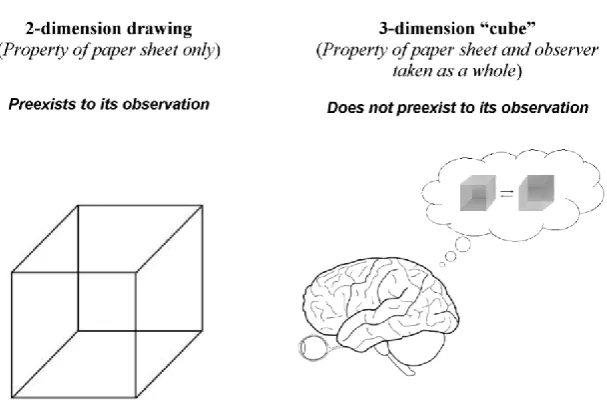
Gestalt psychology. The model has some common points with Gestalt psychology.31 This theory states that the human mind perceives objects as a whole or a form (Gestalt) and not as the simple sum of their constitutive parts. The whole has its own independent existence. Necker cube is an example of the perception of a two-dimension design as a three-dimension Gestalt (Figure 8). Of interest, this three-dimension configuration “exists” only for an observer. Therefore, the “cube” is not a property of the two-dimension sheet alone where a picture has been drawn, but is a property of the sheet and the observer taken as a whole. The three-dimension “cube” does not preexist its observation, but is created at the very moment of its observation.
experimenters could possibly lead to their conditioning. Alternative medicines such as homeopathy or placebo effect are examples where this model could be applied.32 As depicted in this article, the structuration of the observer’s mind by classical conditioning could organize the observations and measurements. In such a situation, the experimenters are trapped into a circular process: they describe what they contribute to construct and they construct what contributes to their description. Moreover, the observation of the expected pattern reinforces the experimenter’s conditioning. Although many other classical explanations are possible, such processes could also be at work in the reproducibility crisis reported in experimental biology, medicine and psychology.33 As we have seen, there is nevertheless a possibility of detecting and avoiding these unintended interferences of the experimenters with the experimental system that they describe. Generalizing the use of an outside supervisor in blind experiments is a method to confirm that an observed relationship is really causal.
9. Conclusion
This psychophysical model allows explaining the results of “memory of water” experiments without referring to water or another local cause. It could be extended to other scientific fields in biology, medicine and psychology when suspecting an experimenter effect.
Figure 8. Necker cube as an example of pattern expectation after learning. Necker cube is a 2-dimensional drawing that we perceive as a 3-2-dimensional volume as a consequence of learning at an early age. Because of the ambiguous drawing, perceptions from top and bottom alternate (only one
of the two patterns can be “seen” at one time). The 2-dimensional drawing is a property of the paper sheet alone, whereas the interaction of the observer with the 2-dimensional drawing literally “creates”
the 3-dimension cube that does not preexist its observation. Similar to Necker cube with top/bottom configurations, direct/reverse relationships are perceived as patterns after learning (through classical conditioning). Both 3-dimensional Necker cube and relationships (between “labels” and system states) are constructs of observer’s mind that considers them in their wholeness and not as the simple
REFERENCES
1. Beauvais F. Ghosts of Molecules – The case of the “memory of water”: Collection Mille Mondes; 2016.
2. Davenas E, Beauvais F, Amara J, Oberbaum M, Robinzon B, Miadonna A, et al. Human basophil degranulation triggered by very dilute antiserum against IgE. Nature 1988;333:816-8.
3. Maddox J. When to believe the unbelievable. Nature 1988;333:787.
4. Schiff M. The Memory of Water: Homoeopathy and the Battle of Ideas in the New Science. London: Thorsons Publishers; 1998.
5. Benveniste J. Ma vérité sur la mémoire de l'eau. Paris: Albin Michel; 2005. 6. Maddox J. Waves caused by extreme dilution. Nature 1988;335:760-3.
7. Maddox J, Randi J, Stewart WW. "High-dilution" experiments a delusion. Nature 1988;334:287-91.
8. Endler PC, Schulte J, Stock-Schroeer B, Stephen S. "Ultra High Dilution 1994" revisited 2015 - the state of follow-up research. Homeopathy 2015;104:223-6.
9. Demangeat JL. Gas nanobubbles and aqueous nanostructures: the crucial role of dynamization. Homeopathy 2015;104:101-15.
10. Del Giudice E, Preparata G, Vitiello G. Water as a free electric dipole laser. Phys Rev Lett 1988;61:1085-8.
11. Elia V, Ausanio G, Gentile F, Germano R, Napoli E, Niccoli M. Experimental evidence of stable water nanostructures in extremely dilute solutions, at standard pressure and temperature. Homeopathy 2014;103:44-50.
12. Van Wassenhoven M, Goyens M, Henry M, Capieaux E, Devos P. Nuclear Magnetic Resonance characterization of traditional homeopathically manufactured copper (Cuprum metallicum) and plant (Gelsemium sempervirens) medicines and controls. Homeopathy 2017;106:223-39.
13. Chikramane PS, Suresh AK, Bellare JR, Kane SG. Extreme homeopathic dilutions retain starting materials: A nanoparticulate perspective. Homeopathy 2010;99:231-42.
14. Aïssa J, Jurgens P, Litime MH, Béhar I, Benveniste J. Electronic transmission of the cholinergic signal. Faseb J 1995;9:A683.
15. Aïssa J, Litime MH, Attias E, Allal A, Benveniste J. Transfer of molecular signals via electronic circuitry. Faseb J 1993;7:A602.
16. Benveniste J, Aïssa J, Litime MH, Tsangaris G, Thomas Y. Transfer of the molecular signal by electronic amplification. Faseb J 1994;8:A398.
17. Benveniste J, Arnoux B, Hadji L. Highly dilute antigen increases coronary flow of isolated heart from immunized guinea-pigs. Faseb J 1992;6:A1610.
18. Benveniste J, Jurgens P, Hsueh W, Aïssa J. Transatlantic transfer of digitized antigen signal by telephone link. J Allergy Clin Immunol 1997;99:S175.
19. Hadji L, Arnoux B, Benveniste J. Effect of dilute histamine on coronary flow of guinea-pig isolated heart. Inhibition by a magnetic field. Faseb J 1991;5:A1583.
20. Benveniste J, Jurgens P, Aïssa J. Digital recording/transmission of the cholinergic signal. Faseb J 1996;10:A1479.
21. Benveniste J, Aïssa J, Guillonnet D. Digital biology: specificity of the digitized molecular signal. Faseb J 1998;12:A412.
22. Beauvais F. Emergence of a signal from background noise in the "memory of water" experiments: how to explain it? Explore (NY) 2012;8:185-96.
24. Rehman I, Mahabadi N, Rehman C. Classical Conditioning. [Updated 2019 Jun 3]. In: StatPearls [Internet]. Treasure Island (FL): StatPearls Publishing; 2019 Jan-. Available from:
https://www.ncbi.nlm.nih.gov/books/NBK470326/. 2019.
25. Beauvais F. “Memory of Water” Without Water: Modeling of Benveniste’s Experiments with a Personalist Interpretation of Probability. Axiomathes 2016;26:329-45.
26. Beauvais F. Description of Benveniste’s experiments using quantum-like probabilities J Sci Explor 2013;27:43-71.
27. Jonas WB, Ives JA, Rollwagen F, Denman DW, Hintz K, Hammer M, et al. Can specific biological signals be digitized? FASEB J 2006;20:23-8.
28. Thomas Y. The history of the Memory of Water. Homeopathy 2007;96:151-7.
29. Benveniste J, Davenas E, Ducot B, Cornillet B, Poitevin B, Spira A. L'agitation de solutions hautement diluées n'induit pas d'activité biologique spécifique. C R Acad Sci II 1991;312:461-6.
30. Breuer T. The impossibility of accurate state self-measurements. Philos Sci 1995;62:197-214. 31. Jakel F, Singh M, Wichmann FA, Herzog MH. An overview of quantitative approaches in
Gestalt perception. Vision research 2016;126:3-8.
32. Beauvais F. Possible contribution of quantum-like correlations to the placebo effect: consequences on blind trials. Theoretical biology & medical modelling 2017;14:12.
33. Baker M. 1,500 scientists lift the lid on reproducibility. Nature 2016;533:452-4.
Funding