Eigen Artificial Neural Networks
Francisco Yepes Barrera1
Abstract
This work has its origin in intuitive physical and statistical considerations. The problem of optimizing an artificial neural network is treated as a physical system, composed of a conservative vector force field. The derived scalar potential is a measure of the potential energy of the network, a function of the distance between predictions and targets.
Starting from some analogies with wave mechanics, the description of the sys-tem is justified with an eigenvalue equation that is a variant of the Schr˜odinger equation, in which the potential is defined by the mutual information between inputs and targets. The weights and parameters of the network, as well as those of the state function, are varied so as to minimize energy, using an equivalent of the variational theorem of wave mechanics. The minimum energy thus obtained implies the principle of minimum mutual information (MinMI). We also propose a definition of the potential work produced by the force field to bring a network from an arbitrary probability distribution to the potential-constrained system, which allows to establish a measure of the complexity of the system. At the end of the discussion we expose a recursive procedure that allows to refine the state function and bypass some initial assumptions, as well as a discussion of some topics in quantum mechanics applied to the formalism, such as the uncertainty principle and the temporal evolution of the system.
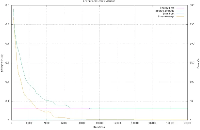
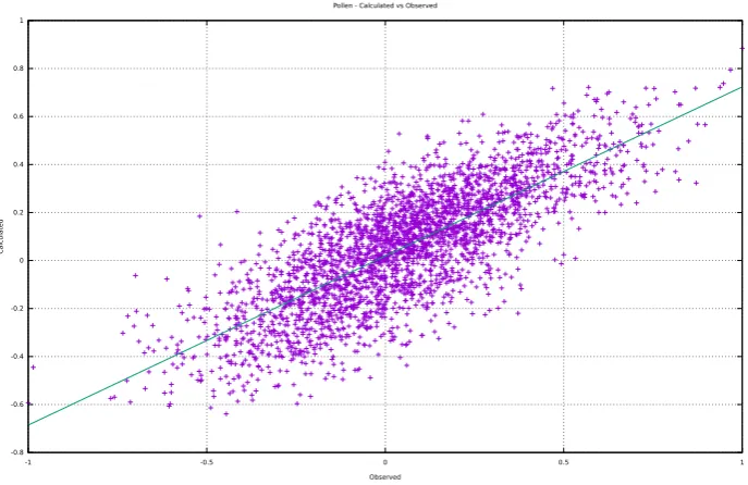
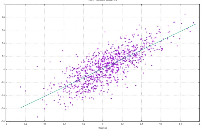
Results demonstrate how the minimization of energy effectively leads to a decrease in the average error between network predictions and targets.
Keywords: Artificial Neural Networks optimization, variational techniques, Minimum Mutual Information Principle, Wave Mechanics, eigenvalue problem.
A note on the symbolism
In the continuation of this work we will represent in bold the set of inde-pendent components of a variable and in italic with subscripts the operations on the single components. In the paper considerations are made and a model is constructed starting from the expected values (mean) of quantities, modeled with appropriate probability densities, and not on the concrete measurements of these quantities. Considering a generic multivariate variableQ,qrepresents the set of components ofQ(number of features) while qi represents each com-ponent being a vector composed of the individual measurementsqij. Similarly, dx = Q
idxi and dt =
Q
ktk represent respectively the differential element of volume in the space of inputs and targets, wherebyR(. . .)dx andR(. . .)dt
express the integration on the whole space whileR
(. . .)dxi and
R
(. . .)dtk the integration on the individual components. In the text, the statistical modeling takes place at the level of the individual components, which in the case of inputs and targets is constructed with probability densities generated from the relative measurements. h. . .imeans expected value.
When not specified, we will implicitly assume that integrals extend to the whole space in the interval [−∞:∞].
1. Introduction
This paper analyzes the problem of optimizing artificial neural networks (ANNs), ie the problem of finding functions y(x; Γ), dependent on matrices of input data x and parameters Γ, such that, given a target t make an optimal mapping betweenxandt[44]. The treatment is limited to pattern recognition problems related to functional approximation of continuous variables, excluding time series analysis and pattern recognition problems involving discrete vari-ables.
The starting point of this paper is made up of some well-known theoretical elements:
1. Generally, the training of an artificial neural network consists in the mini-mization of some error function between the output of the networky(x; Γ) and the target t. In the best case it identify the global minimum of the error; in general it finds local minima. The total of minima compose a discrete set of values.
2. The passage from a prior to a posterior or conditional probability, that is the observation or acquisition of additional knowledge about data, im-plies a collapse of the function that describes the system: the conditional probability calculated with Bayes’ theorem leads to distributions of closer and more localized probabilities than prior ones [11].
3. Starting from the formulation of the mean square error produced by an artificial neural network and considering a set C of targetstk whose dis-tributions are independent
p(t|x) = C
Y
k=1
p(tk|x) (1)
p(t) = C
Y
k=1
p(tk) (2)
wherep(tk|x) is the conditional probability oftk givenxand p(tk) is the marginal probability oftk, it can be shown that
(yk−tk)2≥
(htk|xi −tk)2 (3)
y0k=htk|xi (4) These points have analogies with three theoretical elements underlying wave mechanics [49]:
1. Any physical system described by the Schr˜odinger equation and con-strained by a scalar potentialV(x) leads to a quantization of the energy values, which constitute a discrete set of real values.
2. A quantum-mechanical system is composed by the superposition of several states described by the Schr˜odinger equation, corresponding to as many eigenvalues. The observation of the system causes the collapse of the wave function on one of the states, being only possible to calculate the probability of obtaining the different eigenvalues.
3. When it is not possible to analytically obtain the true wave function Ψ0and the true energyE0 of a quantum-mechanical system, it is possible to use trial functions Ψ, with eigenvaluesE, dependent on a set Γ of parameters. In this case we can find an approximation to Ψ0 and E0 varying Γ and taking into account the variational theorem
(
E=
R
Ψ∗HˆΨdx
R
Ψ∗Ψdx
)
≥E0
Regarding point 3, we can consider the condition (3) as an equivalent of the variational theorem for artificial neural networks.
2. Quantum mechanics and information theory
The starting point of this work consists of some analogies and intuitive con-siderations. Similar analogies based on the structural similarity between the equations that govern some phenomena and Schr¨odinger’s equation are found in other research areas. For example, the Black-Scholes equation for the pricing of options can be interpreted as the Schr¨odinger equation of the free particle [20, 65].
As we will see in the part related to the analysis of the results, empiri-cal evidence in applying the model to some datasets supports the validity of the mathematical formalism detailed in the following sections. However, the premises of this paper suggest a relationship between quantum mechanics and information theory without adequate justification. The rich literature available on this topic mitigates this inadequacy. We will not do a thorough analysis on the matter, but it is worth mentioning some significant works:
1. Kurihara and Uyen Quach [47] analyzed the relationship between proba-bility amplitude in quantum mechanics and information theory.
is a measure of the uncertainty principle. Falaye et al. [23] analyzed the quantum-mechanical probability for ground and excited states through Fisher information, together with the relationship between the uncertainty principle and Cram´er-Rao bound. Entropic uncertainty relations have been discussed by Bialynicki-Birula and Mycielski [10], Coles et al. [19] and Hilgevoord and Uffink [40].
3. Reginatto showed the relationship between information theory and the hydrodynamic formulation of quantum mechanics [62].
4. Braunstein [13] and Cerf and Adami [15] showed how Bell’s inequality can be written in terms of the average information and analyzed from an information-theoretic point of view.
5. Parwani [59] highlights how a link between the linearity of the Schr¨odinger equation and the Lorentz invariance can be obtained starting from information-theoretic arguments. Yuan and Parwani [81] have also demonstrated within nonlinear Schr¨odinger equations how the criterion of minimizing energy is equivalent to maximizing uncertainty, understood in the sense of information theory.
6. Klein [46, 45] showed how Schr¨odinger’s equation can be derived from purely statistical considerations, showing that quantum theory is a sub-structure of classical probabilistic physics.
3. Treatment of the optimization of artificial neural networks as an eigenvalue problem
The analogies highlighted in Section 1 suggest the possibility of dealing with the problem of optimizing artificial neural networks as a physical system.1 These analogies, of course, are not sufficient to justify the treatment of the problem with eigenvalue equations, as happens in the physical systems modeled by the Schr¨odinger equation, and are used in this paper exclusively as a starting point that deserves further study. However it is a line of research that can clarify intimate aspects of the optimization of an artificial neural network and propose a new point of view of this process. We will demonstrate in the following sections that meaningful conclusions can be reached and that the proposed treatment actually allows to optimize artificial neural networks by applying the formalism to some datasets available in literature. A first thought on the model is that it allows to naturally define the energy of the network, a concept already used in some types of ANNs, such as the Hopfield networks in which Lyapunov or energy functions can be derived for binary element networks allowing a complete characterization of their dynamics, and permits to generalize the concept of energy for any type of ANN.
Suppose we can define a conservative force generated by the set of targetst, represented in the input spacexwith a vector field, being N the dimension of
x. In this case we have a scalar functionV(x), called potential, which depends exclusively on theposition2 an that is related to the force as
1In the scientific literature it is possible to find interesting studies of the application of
mathematical physics equations to artificial intelligence [55].
F=−∇V(x) (5) which implies that the potential of the force at a point is proportional to the potential energy possessed by an object at that point due to the presence of the force. The negative sign in the equation (5) means that the force is directed towards the target, where force and potential are minimal, so t generates a force thatattracts thebodies immersed in the field, represented by the average predictions of the network, with an intensity proportional to some function of the distance betweeny(x; Γ) and t. Greater is the error committed by a network in the target prediction, greater is the potential energy of the system, which generates a increase of the force that attracts the system to optimal points, represented by networks whose parameterization allows to obtain predictions of the target with low errors.
Equation (4) highlights how, at the optimum, the output of an artificial neu-ral network is an approximation to the conditional averages or expected values of the targetstgiven the inputx. For a problem of functional approximation like those analyzed in this paper, bothxandtare given by a set of measurements for the problem (dataset), with average values that do not vary over time. We therefore hypothesize a stationary system and an time independent eigenvalue equation, having the same structure as the Schr˜odinger equation
−∇2Ψ(x) +V(x)Ψ(x) =EΨ(x) (6)
where Ψ is the state function of the system (network),V a scalar potential,E the network energy, and a multiplicative constant. Given the mathematical structure of the model, we will refer to the systems obtained from equation (6) asEigen Artificial Neural Networks (EANNs).
Equation (6) implements a parametric model for the ANNs in which the optimization consists in minimizing, on average, the energy of the network, function ofy(x; Γ) and t, modeled by appropriate probability densities and a set of variational parameters Γ. The working hypothesis is that the minimiza-tion of energy through a parameter-dependent trial funcminimiza-tion that makes use of the variational theorem (3) leads, using an appropriate potential, to a reduction of the error committed by the network in the prediction oft. In the continua-tion of this paper we will consider the system governed by the equacontinua-tion (6) a quantum system in all respects, and we will implicitly assume the validity and applicability of the laws of quantum mechanics.
4. The potential
Globerson et al. [37] have studied the stimulus-response relationship in neu-ral populations activity trying to understand what is the amount of information transmitted and have proposed the principle of minimum mutual information (MinMI) between stimulus and response, which we will consider valid in the con-text of artificial neural networks and we will use in the variant of the relationship between x and t.3 An analog principle, from a point of view closer to infor-mation theory, is given by Chen et al. [16, 17], who minimize the error/input
3In the next, we will use the proposal by Globerson et al. translating it into the symbolism
information (EII) corresponding to the mutual information (MI) between the identification error (a measure of the difference between model and target,t−y) and inputx. The intuitive idea behind the proposal of Globerson et al. is that, among all the systems consistent with the partial measured data ofxandt(ie all the systemsythat differ in the set of parameters Γ), the nearest one to the true relationship between stimulus and response is given by the system with lower mutual information, since the systems with relatively high MI contain an additional source of information (noise) while the one with minimal MI contains the information that can be attributed principally only to the measured data and further simplification in terms of MI is not possible. An important impli-cation of this construction is that the MI of the true system (the system in the limit of an infinite number of observations ofxandt) is greater than or equal to the minimum MI possible between all systems consistent with the observations, since the true system will contain an implicit amount of noise that can only be greater than or equal to that of the system with minimum MI.4
So, a function that seems to be a good candidate to be used as potential is the mutual information [80] between input and target, I(t,x), which is a positive quantity and whose minimum corresponds to the minimum potential energy, and therefore to the minimum Kullback-Leibler divergence between the joint probability density of targettand inputxand the marginal probabilities p(t) andp(x)
I(t,x) =
Z Z
p(t|x)p(x) ln
p(t|x)
p(t)
dxdt (7)
In this case, the minimization of energy through a variational state function that satisfies the equation (6) implies the principle of minimum mutual information [28, 36, 37, 82], equivalent to the principle of maximum entropy (MaxEnt) [26, 57, 60, 79] when, as is our case, the marginal densities are known. In the following, in order to make explicit the functional dependence in the expressions of the integrals, we will callIk the function inside the integral in equation (7) relative to a single targettk
Ik(tk,x) =p(tk|x)p(x) ln
p(tk|x)
p(tk)
The scalar potential depends only on the position xand for C targets be-comes
V(x) = C
X
k=1 Z
Ik(tk,x)dtk (8)
The equation (8) assumes a superposition principle, similar to the valid one in the electric field, in which the total potential is given by the sum of the potentials of each of theC targets of the problem, which implies that the field generated by each target tk is independent of the field generated by the other targets.5 In fact it can be shown that this principle is a direct consequence of
4The work of Globerson et al. is proposed in the context of neural coding. Here we
give an interpretation so as to allow a coherent integration within the issues related to the optimization of artificial neural networks.
5This superposition principle, in which the total field generated by a set of sources is equal
the independence of the densities (1) and (2)
R
p(t|x)p(x) lnpp(t(|tx))dt
=R
p(x) lnQC
k=1
p(tk|x) p(tk)
QC
j=1p(tj|x)dt =PC
k=1 R
p(x) lnp(tk|x) p(tk)
QC
j=1p(tj|x)dt =PC
k=1 R
p(tk|x)p(x) lnp(tk|x) p(tk)
dtkR QC
j6=kp(tj|x)dtj6=k =PC
k=1 R
p(tk|x)p(x) lnp(tk|x) p(tk)
dtk
(9)
whereR QC
j6=kp(tj|x)dtj6=k =Q C j6=k
R
p(tj|x)dtj = 1 in the case of normalized probability densities.6 This result has a general character and is independent of the specific functional form given to the probabilitiesp(tk|x) andp(tk).
The conservative field proposed in this paper and the trend for the derived potential and force suggests a qualitative analogy with the physical mechanism of the harmonic oscillator, which in the one-dimensional case has a potential V(x) = 1
2kx
2, which is always positive, and a force given byF
x=−kx(Hooke’s law), where k is the force constant. Higher is the distance from the equilibrium point (x= 0) higher are potential energy and force, the last directed towards the equilibrium point where both, potential and force, vanish. In the quantum formulation there is a non-zero ground state energy (zero-point energy).
Similarly to the harmonic oscillator, the potential (8) is constructed starting from a quantity, the mutual information Ik(tk,x), strictly positive. From the discussion we have done on the work of Globerson et al. at the beginning of this section, the optimal (network) system, that makes the mapping closest to the true relationship between inputs and targets, is the one with the minimum mutual information, which implies the elimination of the structures that are not responsible for the true relationship contained in the measured data. Thus, in the hypotheses of our model, given two networks consisting with observations, the one with the largest error in the target prediction has a greater potential energy (mutual information), being subjected to a higher mean force. Note that for a dataset that contains some unknown relationship between inputs and targets the potential (8) cannot be zero, which would imply p(tk|x) = p(tk) and for the joint probability p(tk,x) = p(tk)p(x), with the absence of a relation (independence) between x and t and therefore the impossibility to make a prediction. Therefore, an expected result for the energy obtained from the application of the potential (8) to the differential equation (6) is a non-zero value for the zero-point energy, that is an energyE >0 for the system at the minimum, and a potential not null.
Considering that the network provides an approximation to the target tk given by a deterministic function yk(x; Γ) with a noise εk, tk = yk +εk, and considering that the error εk is normally distributed with mean zero, the con-ditional probabilityp(tk|x) can be written as [11]
p(tk|x) = 1 (2πχ2
k)1/2 exp
−(yk−tk) 2
2χ2
k
(10)
We can interpret the standard deviationχk of the predictive distribution fortk as an error bar on the mean valueyk. Note thatχk depends onx,χk=χk(x), so χk is not a variational parameter (χk ∈/ Γ). To be able to integrate the differential equation (6) we will consider the vector χ~ constant. We will see at the end of the discussion that it is possible to obtain an expression for χk dependent onx, which allows us to derive a more precise description of the state function.
Writing unconditional probabilities for inputs and targets as Gaussians, we have
p(x) = 1
(2π)N/2|Σ|1/2exp
−1 2(x−~µ)
TX−1
(x−~µ)
p(tk) = 1 (2πθ2
k)1/2 exp
−(tk−ρk) 2
2θ2
k
(11)
Considering the absence of correlation between theN input variables, the prob-abilityp(x) is reduced to
p(x) = N
Y
i=1 1 √
2πσi exp
−(xi−µi) 2
2σ2
i = N Y i=1
Ni (12)
where, in this case, |Σ|1/2 = QN
i=1σi, representing with Ni = N(µi;σi2) the normal distribution with meanµi and varianceσi2relative to the componentxi of the vectorx. The equations (11) and (12) introduce in the model a statistical description of the problem starting from the observed data, through the set of constants~ρ,~θ,~µand~σ. The integration of the equation (8) overtk gives
V(x) = N Y i=1 Ni C X k=1
αkyk2+βkyk+γk
(13)
where
αk = 1 2θ2
k
, βk =−ρk θ2
k
, γk= ρ 2
k+χ2k 2θ2
k
−lnχk √
e θk
(14)
It is known that a linear combination of Gaussians can approximate an arbitrary function. Using a base of dimension P we can write the following expression foryk(x; Γ)
yk(x; Γ) = P
X
p=1
wkpφp(x) +wk0 (15)
where
φp(x) = expn−ξpkx−~ωpk2o= N
Y
i=1
exp−ξp(xi−ωpi)2 (16)
Taking into account the equations (5), (13) and (15) the components of the force,Fi, are given by
Fi = ζQN
i=1Ni PC
k=1 n
xi−µi σ2
i
αkw2
k0+βwk0+γk+ (2αkwk0+βk)PPp=1wkp
h
2ξp(xi−ωpi) +xi−µi σ2
i
i
φp+ αkPP
p=1 PP
q=1wkpwkq h
2ξq(xi−ωqi) + 2ξp(xi−ωpi) +xi−µi σ2
i
i
φpφqo (17) with an expected value for the force given by the Ehrenfest theorem
hFi=−
∂V(x)
∂x
=−
Z
Ψ∗(x)∂V(x)
∂x Ψ(x)dx
5. The state equation
A dimensional analysis of the potential (13) shows that the term αkyk2− βkyk+γk is dimensionless, and therefore its units are determined by the factor |Σ|−1/2. SinceV(x) has been obtained from mutual information, which unit is nat if it is expressed using natural logarithms, we will call the units of|Σ|−1/2
energy nats or enats.7 To maintain the dimensional coherence in the equation (6) we define= σ2x
(2π)N/2|Σ|1/2,
8 where
σ2x∇2= N
X
i=1
σi2 ∂
2
∂x2
i
σ2
x cannot be a constant factor independent of the single components ofxsince in general everyxihas its own units and its own variance. The resulting Hamil-tonian operator
ˆ
H = ˆT + ˆV =− σ 2 x
(2π)N/2|Σ|1/2∇ 2+
N
Y
i=1 Ni
C
X
k=1
αkyk2+βkyk+γk
is real, linear and hermitian. Hermiticity stems from the condition that the average value of energy is a real value, hEi = hE∗i.9 Tˆ and ˆV represent the operators related respectively to the kinetic and potential components of ˆH
ˆ
T =− σ
2 x
(2π)N/2|Σ|1/2∇ 2
7The concrete units of factor|Σ|−1/2are dependent on the problem. The definition of enat
allows to generalize the results.
8This setting makes it possible to incorporate |Σ|−1/2
into the value ofE, but in the continuation we will leave it explicitly indicated.
Calculations show that the ratio between kinetic and potential energy is very large close to the optimum. The factor (2π)−N/2 in the expression oftries to reduce this value in order
to increase the contribution of the potential to the total energy. This choice is arbitrary and has no significant influence in the optimization process, but only in the numerical value ofE.
9In this article we only use real functions, so the hermiticity condition is reduced to the
ˆ V =
N
Y
i=1 Ni
C
X
k=1
αky2k+βkyk+γk
The final state equation is
EΨ =− σ
2 x
(2π)N/2|Σ|1/2∇ 2
Ψ + N
Y
i=1 Ni
C
X
k=1
αkyk2+βkyk+γk
Ψ =hTi+hVi
(18) where thehTiandhVicomponents of the total energyEare the expected values of the kinetic and potential energy respectively. Wanting to make an analogy with wave mechanics, we can say that the equation (18) describes the motion of a particle of mass m = (2π)N/22|Σ|1/2 subject to the potential (13). σ2
x, as happens in quantum mechanics with the Planck constant, has the role of a scale factor: the phenomenon described by the equation (18) is relevant in the range of variance for each single componentxi ofx.
Initially, in the initial phase of this work and in the preliminary tests, we considered an integer factor greater than 1 in the expression of the potential, in the formV(x) =ζPC
k=1 R
Ik(tk,x)dtk. The reason was that at the minimum of energy the potential energy is in general very small compared to kinetic energy, and the expected valuehVicould have little influence in the final result. However, this hypothesis proved to be unfounded for two reasons:
1. it is true that, at min{E}, it occurs hhTVii 1, but the search for this value with the genetic algorithm illustrated in Section 8 demonstrated howhVi is determinant far from the minimum of energy, thus having a fundamental effect in the definition of the energy state of the system;
2. the calculations show how, even in the case of considering ζ 1, the ratio hhTVii remains substantially unchanged, and the overall effect of ζ in this case is to allow expected values for the mutual information smaller than those obtained for ζ = 1. This fact can have a negative effect since it can lead to a minimum of energy where the MI does not correspond to that energy state of the system that is identified with the true relationship that exists between
x andt, and which allows the elimination of the irrelevant superstructures in data, as we have already discussed in Section 4.
We have discussed the role of the operator ˆV: its variation in the space
x implies a force that is directed towards the target where V(x) and F are minimal. The operator ˆT contains the divergence of a gradient in the space x
and represents the divergence of a flow, being a measure of the deviation of the state function at a point respect to the average of the surrounding points. The role of∇2 in the equation (18) is to introduce information about the curvature of Ψ. In neural networks theory a similar role is found in the use of the Hessian matrix of the error function, calculated in the space of weights, in conventional second order optimization techniques.
We will assume a base of dimensionD for the trial function
Ψ(x) = D
X
d=1
with the basis functions developed as a multidimensional Gaussian
ψd(x) = N
Y
i=1
exp−λd(xi−ηid)2 (20)
Theψdfunctions are well-bahaved because they vanish at the infinity and there-fore satisfy the boundary conditions of the problem. As we will see in Section 7.1, Ψ(x) can be related to a probability density. The general form of the basis functions (20) ultimately allows the description of this density as a superposition of Gaussians.
From a point of view of wave mechanics, the justification of the equation (20) can be found in its similarity to the exponential part of a Gaussian Type Orbital (GTO).10The difference of (20) respect to GTOs simplify the integrals calculation. We can interpret λd and ηid as quantities having a similar role, respectively, to the orbital exponent and the center in the GTOs. In some theo-retical frameworks of artificial neural networks equations (19) and (20) explicit the so called Gaussian mixture model.
Using the equation (19), the expected values for energy and for kinetic and potential terms can be written as
hTi=− 1 (2π)N/2|Σ|1/2
Z
Ψ∗σx2∇2Ψdx=− 1 |Σ|1/2
N
X
i=1
σi2 D
X
m=1
D
X
n=1
cmcnTimn
(22)
hVi=
Z
Ψ∗VˆΨdx= C
X
k=1
D
X
m=1
D
X
n=1
C
X
k=1
cmcnVkmn (23)
where
Timn=
Z
ψ∗m∂ψn ∂x2
i dx
Vkmn=
Z
ψm∗ αkyk2+βkyk+γk
N
Y
i=1
Niψndx
10There are two definitions of GTO that lead to equivalent results: cartesian gaussian type
orbital and spherical gaussian type orbital. The general form of a cartesian gaussian type orbital is given by
GαijkR=Nijkα (x−R1)i(y−R2)j(z−R3)kexp
n
−α|r−R|2o (21)
where Nα
ijk is a normalization constant. A spherical gaussian type orbital is instead given
in function of spherical harmonics, which arise from the central nature of the force in the atom and contain the angular dependence of the wave function. The product of GTOs in the formalism of quantum mechanics, as it also happens in the equations that result from the use of the equation (20) in the model proposed in this paper, leads to the calculation of multi-centric integrals.
A proposal of generalization of the equation (20), closer to (21), can be
ψd(x) =N N
Y
i=1
(xi−ηid)νiexp
−λd(xi−ηid)2
Starting from the expected energy value obtained from the equation (18)11
E=
R
Ψ∗HˆΨdx R
Ψ∗Ψdx (24)
and considering the coefficients in equation (19) independent of each other, ∂cm
∂cn =δmn, whereδmnis the Kronecker delta, the Rayleigh-Ritz method leads
to the linear system
X
n
[(Hmn−SmnE)cn] = 0 (25)
where
Hmn=
Z
ψ∗mHψnˆ dx (26)
Smn=
Z
ψ∗mψndx (27)
ConditionSmn=δmncannot be assumed due to the, in general, non-orthonormality of the basis (20). Orthonormal functions can be obtained, for example, with the Gram-Schmidt method or using a set of functions of some hermitian operator.
To obtain a nontrivial solution the determinant of the coefficients have to be zero
det (H−SE) = 0 (28)
which leads to D energies, equal to the size of the base (19). The D energy valuesEd represent an upper limit to the first true energiesE0d of the system. The substitution of every Ed in (25) allows to calculate the D coefficients c of Ψ relative to the state d. The lowest value among Ed represents the global optimum of the problem or fundamental state that leads, in the hypotheses of this paper, to the minimum or global error of the neural network in the prediction of the target t, while the remaining eigenvalues can be interpreted as local minima. It can be shown that the eigenfunctions obtained in this way form an orthogonal set. The variational method we have discussed has a general character and can be applied, in principle, to artificial neural networks of any kind, not bound to any specific functional form foryk.
Using equations (15) and (16) and taking into account the constancy of χ~, the integrals (26) and (27) have the following expressions
Smn=
π
λn+λm
N2 N
Y
i=1 exp
− λmλn λn+λm
(ηim−ηin)2
Hmn = − 2
|Σ|1/2 λmλn λn+λmSmn×
PN
i=1σ2i
h
2 λmλn
λn+λm(ηim−ηin)
2−1i+
ζΛmnP C
k=1γk+ ΛmnP C
k=1βkwk0+ PC
k=1βk PP
p=1wkpΩmnp+ Λmn PC
k=1αkw 2
k0+ 2PC
k=1αkwk0P
P
p=1wkpΩmnp+
PC
k=1αk PP
p=1 PP
q=1wkpwkqΦmnpq
11We will denote the expected value of energy,hEi, simply asE. Although all the functions
where
Λmn = QNi=1√ 1
2σ2
i(λn+λm)+1
×
expn−2σ2i(ηin−ηim)2λmλn+(ηin−µi)2λn+(ηim−µi)2λm
2σ2
i(λn+λm)+1
o
Ωmnp = Q
N i=1
1 √
2σ2
i(ξp+λn+λm)+1
×
exp
2(2σi2(ηinλn+ηimλm)+µi)ξpωpi
2σ2
i(ξp+λn+λm)+1
×
exp
−(2σ
2
i(λn+λm)+1)ξpωpi2+(2σ 2 i(η
2
inλn+η2imλm)+µ2i)ξp
2σ2
i(ξp+λn+λm)+1
×
expn−2σ2i(ηin−ηim)2λnλm+(ηin−µi)2λn+(ηim−µi)2λm
2σ2
i(ξp+λn+λm)+1
oi
Φmnpq = Q
N i=1
1 √
2σ2
i(ξq+ξp+λn+λm)+1
×
exp
2(2σi2(ξpωpi+ηinλn+ηimλm)+µi)ξqωqi−2σ2i(ηin−ηim)2λnλm
2σ2
i(ξq+ξp+λn+λm)+1
×
exp
−(2σ
2
i(ξp+λn+λm)+1)ξqω2qi+(2σ 2
i(ξpω2pi+η 2
inλn+η2imλm)+µ2i)ξq
2σ2
i(ξq+ξp+λn+λm)+1
×
exp
−(2σ
2
i(λn+λm)+1)ξpωpi2−2(2σ 2
i(ηinλn+ηimλm)+µi)ξpωpi
2σ2
i(ξq+ξp+λn+λm)+1
×
exp
−(2σ
2 i(η
2
inλn+η2imλm)+µ2i)ξp+(ηin−µi)2λn+(ηim−µi)2λm
2σ2
i(ξq+ξp+λn+λm)+1
The number of variational parameters of the model,nΓ, is
nΓ=C(P+ 1) + (N+ 1)P+ (D+ 2)N+D+ 2C+ 1 (29)
The energies obtained by the determinant (28) allow to obtain a system of equations resulting from the condition of minimum
∂Ed
∂Γ = 0 (30)
The system (30) is implicit inχk and must be solved in an iterative way, asχk depends onyk which in turn is a function of Γ = Γ(χk).
One of the strengths of the proposed model is the potential possibility of allowing the application quantum mechanics results to the study of neural net-works. An example is constituted of the generalized Hellmann-Feynman theo-rem ∂Ed ∂Γ = Z Ψ∗∂ ˆ H ∂ΓΨdx
whose validity needs to be demonstrated in this context, but whose use seems justified since it can be demonstrated by assuming exclusively the normality of Ψ and the hermiticity of ˆH. Its applicability could help in the calculation of the system (30).
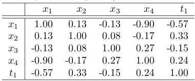
6. System and dataset
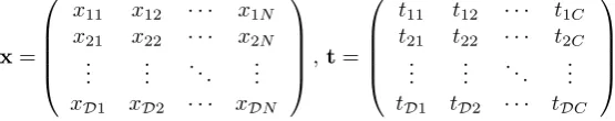
the system, the energy, calculated from the equation (18). The potential energy term can be considered a measure of the distance between the probability distri-butions of inputs and targets [70, 75], given by the mutual information.12 More precisely, the potential energy is the expected value of the mutual information, that is the mean value of MI taking into account all possible values ofxandt. The dataset contains the input and output measurements. We can consider it composed of two matrices, respectivelyxandt, with the following structure
x=
x11 x12 · · · x1N x21 x22 · · · x2N
..
. ... . .. ... xD1 xD2 · · · xDN
,t=
t11 t12 · · · t1C t21 t22 · · · t2C
..
. ... . .. ... tD1 tD2 · · · tDC
whereDrepresents the number of records in the dataset. The interpretation of these matrices is as follows:
1. Matrix x is composed of N vectors xi, equal to the number of columns and which correspond to the number of features of the problem. Vectors xi are represented in italic and not in bold as they represent independent variables in the formalism of the EANNs. A similar discourse can apply to the vectorstk.
2. Matrixtis composed ofCvectorstk, equal to the number of columns and which correspond to the number of output units of the network.
3. Eachxjirepresents the jth record value for featurei.
4. Eachtjk represents the value of thejth record relative to the outputk.
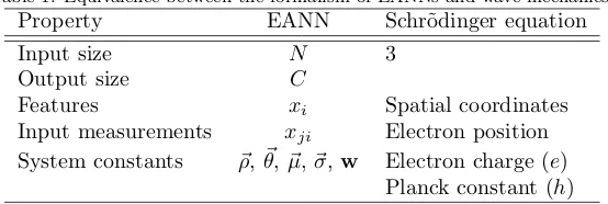
Table 1 illustrates the equivalence between the EANN formalism and quantum mechanics. In particular:
1. Schr¨odinger’s equation describes the motion of the electron in the space subject to a force. Mathematically, the number of independent variables is therefore the number of spatial coordinates. In an EANN an equivalent system would be represented by a problem withN = 3. This constitutes a substantial difference between the two models, since in an EANN the value ofN is not fixed but problem-dependent.
2. The different electron positions in a quantum system are equivalent to the individual measurementsxjionce the target is observed.
3. The probability of finding the electron in a region of space is ultimately defined by the wave function. Similarly, in an EANN the probability of making a measurement within a region in the feature space after observing the target is related to the system state function, as we will analyze in the Section 7.1.
4. Both models depend on a series of constant characteristics of the system: electron charge and Planck constant in the Schr˜odinger equation,~ρ,~θ,~µ, ~
σew in an EANN.
12The properties of mutual information, such as symmetry, allow us to consider it as a
Table 1: Equivalence between the formalism of EANNs and wave mechanics.
Property EANN Schr˜odinger equation
Input size N 3
Output size C
Features xi Spatial coordinates
Input measurements xji Electron position
System constants ~ρ,~θ,µ~,~σ,w Electron charge (e) Planck constant (h)
7. Interpretation of the model
7.1. Interpretation of the state function
The model we have proposed contains three main weaknesses: 1) the nor-mality of the marginal densities p(x) and p(t); 2) the absence of correlation between theN components of the input x; 3) the constancy of the vector χ~. The following discussion tries to analyze the third point.
Similarly to wave mechanics an the Born rule, we can interpret Ψ as a probability amplitude and the square module of Ψ as a probability density. In this case, the Laplacian operator in equation (18) models a probability flow. Given that we have obtained Ψ from a statistical description of a set of known targets, we can assume that |Ψ|2 represents the conditional probability of x
giventsubject to the set of parameters Γ
p(x|t,Γ) =|Ψ(x)|2 (31)
where |Ψ|2dx represents the probability, given t, of finding the input between
xandx+dx. In this interpretation Ψ is a conditional probability amplitude. A fundamental aspect of this paper is that this interpretation of |Ψ(x)|2 as conditional probability is to be understood in a classical statistical sense, which allows to connect the quantum probabilities of the formalism of the EANNs with fundamental statistical results in neural networks and Bayesian statistics, such as Bayes’ theorem. This view is in agreement with the work of some authors in quantum physics, who have underlined how the interpretation of Born’s rule as a classical conditional probability is the connection that links quantum probabilities with experience [42].13 Given the relevance of this point of view in the mathematical treatment that follows, we will make a hypothetical example that in our opinion can better clarify this aspect.
13The conditional nature of quantum probability also appears in other contexts. In the
formalism of Bohmian Mechanics, consider, for example, a particular particle with degree of freedomx. We can divide the generic configuration point q={x, y}, where y denotes the coordinates of other particles, i.e., degrees of freedom from outside the subsystem of interest. We then define the conditional wave function (CWF) for the particle as follows:
φ(x, t) = Ψ(q, t)|y=Y(t)= Ψ [x, Y(t), t]
That is, the CWF for one particle is simply the universal wave function, evaluated at the actual positionsY(t) of the other particles [56].
Consider a system consisting of a hydrogen-like atom, with a single electron. Suppose that this system is located in a universe, different from our universe, in which the following conditions occur:
1. Schr¨odinger’s equation is still a valid description of the system; 2. the potential has the known expressionV =−Ze2
r , whereZ is the number of protons in the nucleus of the atom (atomic number), e the charge of the electron andr the distance between proton and electron;
3. the electron charge is constant given a system, but has different values for different systems;
4. only a value ofecan be used in the Schr¨odinger equation;
5. eis dependent on the system for which it is uniquely defined, but is inde-pendent of spatial coordinates and time;
6. the numerical values for energy and other properties of the atom obtained with differentevalues are different.
7. different physicists will agree in the choice of e. However, a laboratory measurement campaign is required to identify its value.
8. It is not possible to derive the value ofeused for a system from the energy and state function calculated for that system.
Imagine a physicist applying Schr¨odinger’s equation with a givenevalue for the electron charge, obtaining a spatial probability density of the electron|Ψ(x)|2. Sinceeis not unique and cannot be obtained through a logical or mathematical reasoning but only from laboratory measurements, our physicist will have to indicate which value fore he used in his calculations, in order to allow others scientists to repeat his work. So, he will have to say that he got an expression for|Ψ(x)|2 andE given a certain value fore, for example writing
|Ψ(x|e)|2
This notation underlines the conditional character of the electron spatial proba-bility density. Since in our universe the electron charge is constant in all physical systems and the choice of its value is unique, we can simply write |Ψ(x)|2. In a EANNs the probability density in the input space |Ψ(x)|2 is obtained from a potential that contains constants (αk, βk, γk) calculated from a conditional probability density (p(t|x)) and marginal densities (p(x), p(t)) dependent on the target of the problem.
The character of|Ψ(x)|2 as a classical probability allows to relate the equa-tion (31) with the condiequa-tional probabilityp(t|x) through Bayes’ theorem
p(x|t) =p(t|x)p(x)
p(t) (32)
Since we considered theC targets independent, using the expressions (10) and (31) into (32), separating variables and integrating over tk, assuming that at the optimum is satisfied the conditionθk> χk, we have
|Ψ(x)|2 p(x) =
C
Y
k=1 s
2π θ2
k−χ
2
k θk2exp
(yk(x)−ρk)2 2 (θ2
k−χ
2
k)
which leads to an implicit equation in χk. For networks with a single output, C= 1, we have
χ(τ+1)= v u u
tθ2−2πθ4
p(x)2 Ψ(τ)
4exp (
(y−ρ)2
θ2−χ2 (τ)
)
(33)
where Ψ, y andχ are functions of x. The equation (33) allows in principle an iterative procedure which, starting from the constant initial value χ(0) which leads to a state function Ψ(0), through the resolution of the system (25) permits to calculate successive corrections of Ψ.
7.2. Superposition of states and probability
As we said in Section 5 the basis functions (20) are not necessarily orthog-onal, which forces to calculate the overlap integrals given that in this case Smn 6= δmn, where δmn is the Kronecker delta. The basis functions can be made orthogonal or a set of functions of some hermitian operator can be cho-sen, which can be demonstrate to form a complete orthogonal basis set. In the case of a function (19) result of the linear combination of single orthonormal states, the coefficient cm represents the probability amplitudehψm|Ψiof state m
hψm|Ψi= D
X
d=1
cd
Z
ψm∗ψddx= D
X
d=1
cdδdm=cm
being in this casePD
d=1|cd|
2
= 1 and |cd|
2
the prior probability of the stated.
7.3. Work and complexity
From a physical point of view, the motion of a particle within a conservative force field implies a potential difference and the associated concept of work, done by the force field or carried out by an external force. In physical conservative fields, work,W, is defined as the minus difference between the potential energy of a body subject to the force field and that possessed by the body at a an arbitrary reference point, W = −∆V(x). In some cases of central forces, as in the electrostatic or gravitational ones, the reference point is located at an infinite distance from the source where, given the dependence of V on 1r, the potential energy is zero.
Consider a neural network immersed in the field generated by the targets, as described in the previous sections, and which we will call bounded system. We can consider this system as the result of the trajectory followed by a single network with respect to a reference point as starting point. The definition of potential given in Section 4 allows to calculate a potential difference between both points, which implies physical work carried out by the force field or pro-vided by an external force. In the latter case, it may be possible to arrive at a situation where the end point of the process is the unbounded system (free system), not subject to the influence of the field generated by the targets. In this case, the amount of energy provided to the system is an analogue of the ionization energy in an atom.
however, the system evolves towards a greater potential configuration that can only be achieved through the action of an external force. The potential energy is one of the components of the total energy and a decrease in the potential energy does not necessarily imply a decrease of the total energy, but for a stable constrained system the potential of the final state will be lower than the potential of the initial state, represented by the reference point, ifW >0. From these considerations, a good reference point should have the following two properties:
1. have a maximum value with respect to the potential of any system that can be modeled by the equation (18);
2. be independent of the system.
Some well-known basic results from information theory allow to define an upper limit for mutual information. From the general relations that link mutual infor-mation, differential entropy, conditional differential entropy and joint differential entropy, we have the following equivalent expressions for a targettk
Z Z
Ik(tk,x)dtkdx=h(tk)−h(tk|x) =h(x)−h(x|tk)≥0 (34)
Z Z
Ik(tk,x)dtkdx=h(tk) +h(x)−h(tk,x)≥0 (35)
In the case thath(tk)>0, h(x)>0 we can write the following inequalities
Z Z
Ik(tk,x)dtkdx<
h(tk)
h(x) (36)
Equation (36) allows to postulate an equivalent condition which constitutes an upper limit for the expected value of the potential energy given the expected value for differential entropies
hVi<
hh(tk)i
hh(x)i (37)
wherehh(tk)iandhh(x)iare given by
hh(tk)i=
Z Z
Ψ∗h(tk)Ψdtkdx
hh(x)i=
Z
Ψ∗h(x)Ψdx
Consider a system defined by a state function Ψ0in which inputs and targets are independent
p(t,x) =p(t)p(x)
Such a system has zero mutual information. Assuming valid the interpretation we gave in the Section 7.1 of the square of the state function as conditional densityp(x|t), together with the equation (34), callingh0the differential entropy of the system, we have
h|Ψ0| 2
=h0(x)
This system is not bound and we will call it free system, in analogy with that of the free particle in quantum mechanics. In our model it is described by the following state equation
− σ
2 x
(2π)N/2|Σ|1/2∇ 2Ψ
0=EΨ0
The multidimensional problem can be reduced toN one-dimensional problems
Ψ0(x) =
N
Y
i=1
Aiψ0(xi) =A N
Y
i=1
ψ0(xi) (38)
which gives an energy
E= N
X
i=1
Ei
and where A is the normalization constant. There are two solutions for the one-dimensional stationary system
ψ±0(xi) =A±i exp
±i
s
(2π)1/2Ei
σi xi
(39)
where E is not quantized and any energy satisfying E ≥ 0 is allowed. The previous equation corresponds to two plane waves, one moving to the right and the other to the left of the xi axis. The general solution can be written as a linear combination of both solutions.
The normalization of this system is problematic because the state function cannot be integrated and the normalization constant can only be obtained con-sidering a limited interval ∆, but the probability in a differential element on this interval can be calculated. Taking any of the solutions (39)
Z ∆
|ψ0(xi)|2 dxi=A2i
Z ∆
exp
±i
s
(2π)1/2Ei
σi xi
exp
∓i
s
(2π)1/2Ei
σi xi
dxi= 1
Ai= 1 √
∆
|ψ0(xi)|2dxi = ψ
∗
0(xi)ψ0(xi)dxi
R
∆ψ
∗
0(xi)ψ0(xi)dxi
= A2 iexp ( ±ii r
(2π)1/2Ei σi xi
) exp
(
∓i
r
(2π)1/2Ei σi xi
) dxi A2 i R ∆exp ( ±i r
(2π)1/2Ei σi xi
) exp
(
∓i
r
(2π)1/2Ei σi xi
) dxi
= dxi
∆
so the probability density is constant in all points of the interval ∆ and equal to 1
∆, and |ψ0(xi)| 2
is the density of the uniform distribution.14 Since the total state function is the product of the single one-dimensional functions, if the normalization interval (equal to the integration domain that we used) is the same for all the inputs, we have
|Ψ0| 2
= 1
∆N with a differential entropy given by
h0(x) =h
|Ψ0|2
=−
Z ∆
1 ∆N ln
1
∆N
dx=Nln ∆ = N
X
i=1
h0(xi) (40)
Equation (40) expresses the maximum differential entropy considering all pos-sible probability distributions of systems that are solution of the equation (18), equal to the entropy of the conditional probability density given by the square of the state function for the free system. This maximum value and its derivation from a density of probability independent of any system with non-zero poten-tial, allow its choice as a reference value for the calculation of the potential difference. The last equality is a consequence of the factorization of the total state function (38), and expresses the multivariate differential entropy as the sum of the single univariate entropies, which is maximum with respect to each joint differential entropy and indicates independence of the variablesxi. Given the constancy of h0(x), for a normalized state function Ψ0 in the interval ∆, the expected value of the differential entropy for the free system is
hh0(x)i=Nln ∆
Considering an initial state represented by the reference point and a final state given by the potential calculated for a proposal of solution y(x; Γ), work is given by
W =−∆V =h|Ψ0| 2
− hVi=Nln ∆− hVi (41)
ForW >0, equation (41) explains the work, in enats, done by the force field to pass from a neural network that makes uniformly distributed predictions to a network that makes an approximation to the densityp(t|x). Conversely, using a terminology proper of atomic physics, equation (41) expresses the work that must be done on the system in order to pass from the bounded system to the
14This is because the state function has no boundary conditions, that is, it does not cancel
free system, the last represented by a network that makes uniformly distributed predictions.
Consider the following equivalent expression for equation (41), obtainable for Gaussian and normalized probability densities
W =−
Z Z
Ψ∗(x)p(t,x) ln
p(t,x)
p(t)p(x) ∆N
Ψ(x)dtdx (42)
In equation (42) ∆N has the role of a scaling factor, similar to the functionm(x) in the differential entropy as proposed by Jaynes and Guia¸su [3, 4, 66, 38]. From this point of view, W is scale invariant, provided that hVi and h|Ψ0|
2 are measured on the same interval, and represents a variation of information, that is, the reduction in the amount of uncertainty in the prediction of the target through observing input with respect to a reference level given byh|Ψ0|
2 . In this interpretation, where we can considerW as a difference in the information content between the initial and final states of a process,h|Ψ0|
2
is the entropy of an a priori probability and (41) is the definiton of self-organization [24, 25, 33, 50, 67]
S=Ii− If
whereIi is the information of the initial state andIf is the information of the final state, represented by the expected value for the potential energy at the optimum. In a normalized version ofS we have
S= 1− hVi
Nln ∆ (43)
This implies that self-organization occurs (S>0) if the process reduces informa-tion, i.e. Ii>If. If the process generates more information,S <0, emergence occurs. Emergence is a concept complementary to the self-organization and is proportional to the ratio of information generated by a process with respect the maximum information
E= If Ii
= hVi
Nln ∆ (44)
S= 1− E
where 0 ≤[E,S]≤1. The minimum energy of the system implies a potential energy which is equivalent to the most self-organized system. S = 1 implies hVi= 0 and corresponds to a system where input and target are independent, that as we discussed is an unexpected result. So, at the optimum, for a bounded system, we will haveS <1.
L´opez-Ru´ız et al. [50] defined complexity as C=SE
From equations (43) and (44), we have
C= hVi Nln ∆
1− hVi Nln ∆
(45)
7.4. Role of kinetic energy
The MinMI principle provides a criterion that determines how the identi-fication of an optimal neural structure for a given problem can be found in the minimum of mutual information between inputs and targets. However, the equation (18) contains elements other than the term for mutual information, result of having taken without justification an eigenvalue equation having the same structure as the Schr¨odinger equation. The obvious question is: why not just minimizeI(t,x)?
As empirical verification has been minimized the mutual information con-taining a variational function given by equation (15) and a set of normal prob-ability densities, as described in Section 4. This test showed that it’s possible to found a set of parameters Γ that produce values for potential very small, close to zero. However, networks obtained in this way do not produce a sig-nificant correlation between the values of MI and the error in the prediction of targets. The reason for this result has already been commented in the previ-ous sections: I(tk,x) = 0 implies p(tk,x) = p(tk)p(x), independence between inputs and targets, and then the impossibility to build a predictive model. It is necessary additional information that allows to identify the minimum of mu-tual information which constitutes a valid relation between data and represents an approximation to the true relationship between inputs and targets. This additional information is provided by the Laplacian in the kinetic energy term. Perhaps the best way to understand the meaning of the Laplacian is through a hydrodynamic analogy. Consider a function ϕ as the scalar potential of a irrotational compressible fluid.15 It is possible to define the velocity field of the fluid as the gradient of the scalar potential,v =∇ϕ, which is called potential flow. In this case, the Laplacian of the scalar potential is nothing more than the divergence of the flow. For∇2ϕ6= 0 in a certain point, then there exist an acceleration of the potential field. In this sense the Laplacian can be seen as a
"driving force".16 Furthermore, the Laplacian of a function at one point gives the difference between the function value at that point and the average of the function values in the infinitesimal neighborhood. Since the difference of the average of surrounding and the point itself is actually related to the curvature, the driving force can be considered as curvature induced force. In this way,∇2Ψ is the divergence of a gradient in the space of inputs and then may be associated with the divergence of a flow given by the gradient of the probability amplitude, which can be considered a diffusive term that conditioning the concentration of the conditional measurements xij [69] and ultimately the probability |Ψ|2. In this sense, the kinetic term of the equation 18) expresses a constraint to the potential energy, which must be minimized compatibly with a distribution of the conditional probability of the measurements in the spacex.
To understand the nature of this constraint we analyze the mathematical
15Link between wave mechanics and hydrodynamics is well known since the Madelung’s
derivations and related work, that show how Schr¨odinger’s equation in quantum mechanics can be converted into the Euler equations for irrotational compressible flow [18, 51, 72, 73, 74]. However, the discussion in the text is simply a qualitative analogy in order to understand the role of the Laplacian.
16This driving force has not to be confused with the force in classical mechanics, which is
form of the kinetic term. By integrating the equation (22) overxwe have
hTi = − 2
(2π)N/2|Σ|1/2
PN
i=1σi PD
m=1 PD
n=1cmcn
λmλn λm+λn
π λm+λn
N2
×
h
2 λmλn
λm+λn(ηim−ηin)
2−1iQN i=1exp
n
− λmλn
λm+λn(ηim−ηin)
2o (46) The sign of every term of the double sum on (m, n) is given by the product cmcnh2 λmλn
λm+λn(ηim−ηin)
2−1i. Since experimentally it is found that the ex-pected value of the kinetic energy is positive for all the datasets studied and
since− 2
(2π)N/2|Σ|1/2 <0, there is a net effect given by the terms for which this
product is negative which leads to the condition
− 2
(2π)N/2|Σ|1/2
−cmcn
2 λmλn
λm+λn(ηim−ηin)
2 −1
>0
and
λmλn
λm+λn(ηim−ηin)
2> 1
2 (47)
We study the variation of the kinetic energy as a function of the behavior of the following two factors present in the equation ((46), where we have separated the contribution of thei-th feature from those for whichj6=i
f1=
N
Y
j6=i exp
− λmλn
λm+λn(ηjm−ηjn)
2
(48)
f2=
2 λmλn
λm+λn(ηim−ηin)
2−1
exp
− λmλn
λm+λn(ηim−ηin)
2
(49)
In relation tof1,hTidecreases with the increase of λλmm+λλnn and distance (ηjm− ηjn)2. If we consider the λ parameter as a measure of the variance σ2
λ =
1 2λ associated with the correspondent Gaussian, we have λmλn
λm+λn =
1 2(σ2
m+σ2n) and
the equality
exp
− λmλn
λm+λn(ηjm−ηjn)
2 = exp 2 σ 2
m+σn2 (ηjm−ηjn)2
The minimization of hTi therefore leads to a decrease in dispersion and an increase in the centroids distance, or in other words to the localization and separation of the Gaussians. We can consider this behavior an equivalent of the Davies-Bouldin index, which expresses the optimal balance between disper-sion and separation in clustering algorithms [76, 78]. The issue has also been extensively studied in the context of RBF networks [9, 8, 52, 53, 77].
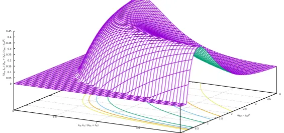
For f2 the behavior is more complex. Figure 1 contains the graphic repre-sentation of the surface given byf2 with the points that satisfy the condition (47). The domains used for independent variables reflect the limits used in the tests:
• λ∈[0 : 4], so λmλn
Figure 1:f2=
h
2 λmλn
λm+λn(ηim−ηin)
2−1iexpn− λmλn
λm+λn(ηim−ηin)
2o
• η ∈[−1 : 1] (the limits of the normalization range ∆), so (ηim−ηin)2∈ [0 : 4].
The qualitative trend of the kinetic energy can be summarized as follows:
1. for large values of λmλn
λm+λn (high values for
1 2(σ2
m+σn2)
),hTimainly decreases proportionally to the distance (ηim−ηin)2. We have a behavior similar to that discussed forf1;
2. for small values of λmλn
λm+λn (low values for
1 2(σ2
m+σn2)),hTidecreases inversely
proportional to the distance (ηim−ηin)2.
For high values of λmλn
λm+λn there are very localized Gaussians whose centers must
be as far apart as possible so as to obtain a good representation of the entire domain of the dataset. For low values of λmλn
λm+λn, however, the Gaussians are very
wide and their centers must be relatively close so as not to lose part of their descriptive capacity, which happens, for example, if the centroids are at the limits of the normalization range. The predominant effect of the productf1f2 implies a decrease ofhTiwith the increase of the localization and the separation of the Gaussians that compose the basis functionsψdof the state function, with a small modulation for low values of λmλn
λm+λn as previously discussed. Note that
7.5. Operators
All the quantities of interest in the model described can be calculated, as happens in quantum mechanics, through the application of suitable operators. However, it must be taken into consideration that the values of the set of varia-tional parameters Γ obtained in the minimization of energy are not, in general, valid for other observables when using trial functions that are not the true eigenfunction of the system. This does not invalidate the results obtained in this section, in which we propose general expressions whose correctness in the numerical results is subject to the use of the correct values of the parameters Γ for each observable under study.
7.5.1. Expected value for outputyk
Considering equation (15) and (19) we can write the following expression for the expected value ofyk
hyki=
Z
yk|Ψ|2 dx= P X p=1 D X d=1 D X l=1 wkpcdcl Z
φpψdψldx+wk0
Using equations (16) and (20) we obtain the final result
hyki = wk0+P
P p=1
PD
d=1 PD
l=1wkpcdcl
π ξp+λl+λd
N2
×
QN
i=1exp
−ξp[λl(ωpi−ηil)2+λd(ωpi−ηid)2]+λdλl(ηil−ηid)2 ξp+λl+λd
7.5.2. Expected value for xi
The expected value of a component xi of of the conditional probability |Ψ(x)|2 is given by
hxii=
Z
xi|Ψ|
2
dx= D X d=1 D X l=1
cdcl
Z
xiψdψldx
and using equations (16) and (20)
hxii= D X d=1 D X l=1
cdcl(λdηid+λlηil) π
N 2
(λd+λl)N+22 N Y i=1 exp − λdλl λd+λl
(ηil−ηid)2
7.5.3. Expected value for the variance ofxi Variance for xi is given by
(∆xi)2=
x2i
− hxii
2
7.6. Uncertainty principle
In this section we make an analysis of the possible validity of the uncertainty principle within the EANNs. For simplicity we will consider in the treatment the one-dimensional case, that is a system composed by a neural network with a single inputx.
From a direct comparison between the differential equation describing the physical behavior of the EANNs and the Schr˜odinger equation, we postulate the following expression for the operator ˆp2
ˆ
p2x=−σ2x∇2 (50)
The negative sign allows to obtain positive kinetic energies, as has been con-firmed by the experiments detailed in Section 8, and necessarily leads to an expression for momentum operator ˆpxwhich contains the imaginary unit
ˆ px= σx
i ∇ (51)
According to the laws of probability, the variances (∆x)2and (∆px)2related to the observablesxandpxcan be written as [49]
(∆x)2=
(x− hxi)2
=
x2
− hxi2=
Z
Ψ∗(ˆx− hxi)2Ψdx (52)
(∆px)2=
(px− hpxi)2
=
p2x
− hpxi2=
Z
Ψ∗(ˆpx− hpxi)2Ψdx (53)
Equations (52) and (53) are in fact definitions of a variance. In particular, the equation (52) is the expected value of the quadratic deviation of the variablex measured against a conditional probability density given by the square of the state function, and should not be confused withσ2
x, which is the variance given by the marginal probability density of x. Taking into account the definition of expected value and the mathematical properties of Schwartz’s inequality, for the product of standard deviations we have [14, 63]
∆x∆px≥1 2 Z
Ψ∗[ˆx,pxˆ ]Ψdx
(54)
where [ˆx,pxˆ ] is the commutator for position, ˆx, and momentum, ˆpx, operators. If we consider valid the rules of commutation in quantum mechanics and their meaning as the possibility or not of measuring with arbitrary precision the values of conjugated variables, then there exits an uncertainty relationship also in the EANNs. The reason lies in the fact that any operator composed of a first derivative does not commute with the position operator. By defining the operator ˆD= dxd, the commutator with ˆxgives rise, as is known, to
ˆ
Dxˆ= ˆ1 + ˆxDˆ
d
dx,ˆx
= ˆDxˆ−xˆDˆ = ˆ1
where ˆ1 is the unit operator. In our case, for the position-momentum commu-tator, taking into account that [ˆx,pˆx] =−[ˆpx,xˆ], we have
[ˆx,pˆx] =
ˆ x,σx i ∂ ∂x =σx i ˆ x, ∂ ∂x
=−σx i
∂
∂x,xˆ
=−σx i =iσx
Finally, from the equation (54)
∆x∆px≥ 1 2 Z
Ψ∗iσxΨdx
= σx 2 |i|
Z
Ψ∗Ψdx
∆x∆px≥ σx
Assuming therefore an operator of the form (51) and taking into account very general considerations, we obtain an equivalent of the uncertainty principle for the EANNs. This result is not surprising given the mathematical equivalence with the Schr˜odinger equation.
It is possible to generalize this result for pairs of generic conjugated variables if one assumes the validity for the EANN of some classical results in quantum mechanics, which however needs formal verification. If the equation (18) governs the behavior of a true quantum system in which not all pairs of variables com-mute, we can hypothesize the existence of a classic system in which all variables instead commute. In this context, from a quantum point of view an equivalent of Dirac’s proposal for pairs of variables (f, g) is
[ ˆf ,gˆ] =iσx{f, g} where{f, g}is the Poisson bracket between f andg.
From a physical point of view, the equation (54) is a formalization of the im-possibility of simultaneously measuring position and momentum with arbitrary precision, ie the fact that the variance in the position is subject to a kinematic constraint [6]. Equivalently, within non-commutative algebras, it makes ex-plicit the fact that position and momentum cannot be made independent from a statistical point of view, constituting a limit to a priori knowledge regarding observable statistics and their predictability. Equation (55) highlights how the product in the uncertainties or variances of two non-independent observables cannot be less than a certain minimum value, which is related to the standard deviation of the marginal density of the dataset.
Equation (55) can be derived from purely statistical considerations. Start-ing from the inequality proposed independently by Bourret [12], Everett [22], Hirschman [41] and Leipnick [48], satisfied by each functionψ and its Fourier transformψe
−
Z
|ψ(x)|2ln|ψ(x)|2 dx−
Z ψe(px)
2
ln
ψe(px)
2
dpx=h(x) +h(px)≥1 + lnπ
Beckner [7] and Bialinicki-Birula and Micielski [10] demonstrated
h(x) +h(px)≥ln(πeσx) (56) where we assumed the equivalence~≡σx. Since the differential entropy of the normal probability density is maximum among all distributions with the same variance, for a generic probability densityf(z) we can write the inequality
h(z)≤ln(√2πe∆z) (57)
Substituting (57) in (56) we have
∆x∆p≥ 1
2πeexp{h(x) +h(px)} ≥ σx
2
It is worth mentioning that the equation (56) is derived from mathematical properties and acquires the form of the text at the end of the proof, when considering a concrete expression forpx.