Assessment of Adaptive Step Size INC MPPT Algorithm for
Standalone and Grid Connected PV Applications
Shubham Mishra
Electrical Engineering Department, Shri Ramswaroop Memorial University Lucknow, India
ABSTRACT
In this paper, photovoltaic (PV) plant module is used for compensating power demand in both cases i.e. standalone
and grid connected system. This task is performed by an advanced incremental conductance MPPT algorithm,
which provides a current or voltage reference to the converter.
The paper provides two simulink based designs; one for standalone system supplying DC load and another for grid
connected full-bridge pulse width-modulated inverter that is cascaded and injects synchronized AC current to the
grid. In the grid connected system a current controller along with voltage regulator is used to regulate the grid
current. A PV module with boost converter is demonstrated for standalone system and for a 100kW grid. Simulation
results verify the validity and performance of the circuit operations, MPPT control algorithm.
Keywords—
Grid, Incremental conductance, MPPT Photovoltaic array, Standalone system.
I INTRODUCTION
The increasing power stipulate joined by the option of condensed deliver of predictable fuels, evidenced via fuel calamity, beside by rising concerns regarding ecological maintenance, have motivated study with growth of another power sources to be cleaner, be renewable, with make small ecological contact. By the year 2030, the annual reduction rate of CO2 due to the usage of PV cells may be around 1 Gton/year, which is equivalent to India‟s total
emissions in 2004 or the emission of 300 coal plants [1].
competence with too increases the mass plus load of the circuit. In sort to conquer the restrictions a boost kind of inverter can be engaged thus dipping the on the whole gain constraint of the dc-dc converters [6].
The dc voltage output of photovoltaic (PV) unit lower than the peak grid voltage, and their output voltage varies in a wide range according to various operation conditions. Succession link of some such modules helps to enlarge their yield voltage hence like near utilize a buck-type grid-connected inverter designed for power translation. Though, this technique can decrease the effort power set collection. Moreover, sequence link of PV modules might lessen the on the whole competence of the PV array (a PV array consists of some PV modules), as entity modules be successively in dissimilar circumstances [7]. For boosting PV yield voltage in sort near contain the buck-type grid-connected inverter, a two-stage topology to boosts the PV voltage via a dc–dc converter in the initial phase also next inverts it keen on ac voltages with the succeeding step be reported during prior journalism. In [7], a cascaded configuration the entity PV voltage is stepped up to a advanced component yield voltage by make up an collection yield voltage like the front-end of a buck-type grid-connected inverter.
The present paper deals with both the issues of solar PV systems operating in standalone mode to provide power to domestic loads in locations wherein grid is not available and also to the grid connected system. This manuscript presents a customized incremental conductance MPPT technique practical into a double-stage grid-connected PV scheme. To let alone voltage fall down phenomena, the least step span near amend the orientation significance of the yield power vary according near the tracking path. Here this adapted technique, if the yield power of PV panels is detected near be lessening fast, the controller resolve guess to a step change of solar radiation occurs, also next, retune the orientation yield power of the inverter according near the current PV yield power.
II MODELING OF PV DEVICES
2.1
Ideal PV Cell
A single PV cell cannot produce enough power and cannot be used in majority of applications [8]. In order to get power that is practicable for most of the applications individual cells are connected in series/parallel configurations.
2.2
PV
Module Model in MATLAB-Simulink
The block diagram of the MATLAB-Simulink-based PV module model is shown in Fig. 1, where the proposed model is designed with irradiance as input and three outputs. Ir is irradiance (W/m2), I_PV isthe output current of PV module, V_PV is the output voltage of the PV module, and Idiode is the output diode current of the PV module.
KD135GX-LP.HereIph is the controlled current source used for simulating the output current of the PV module. A
bypass diode is connected in parallel with this controlled current source Iph. For the sake of convenience, all
components in fig. 1(a) are incorporated into a subsystem block of PV array are shown in 1(b) using in following steps.
1(a)
1(b)
Figure 1. PV module model in MATLAB-Simulink (a) Block diagram of the PV module model. (b)
PV module model in a subsystem.
Table1
Parameters of a PV module
Parameter Value
Short-circuit current [A] ISC= 8.36955
Open-circuit voltage [V] VOC= 22.0999
Maximum Power point voltage[V] Vmp = 17.7
Maximum Power point current[A] Imp= 7.62959
Series resistance(Ω) Rs= 0.10593
Parallel resistance(Ω) Rp= 142.84
Photo-generated current[A] Iph= 5.3758
Diode quality factor Qd=1.5
Sample time(sec) t= 1e-6
Number of cells per module N=36
Number of series-connected modules per string Nser=4
Number of parallel strings Npar=1
Step 1: Enclose the blocks and connect lines in fig. 1(a) within a bounding box.
Step 2: Choose the option of create subsystem from the Edit menu.
MATLAB-Simulink replaces the selected blocks with a subsystem block, which is shown in Fig. 1(b).The subsystem block in Fig. 1(b) will be a basic PV module mode of MATLAB-Simulink in this paper. In the subsystem block, port of 1 + is the positive terminal of the PV module, port 2is the negative terminal of the PV module, port 1 of Ir is the incidence irradiance of the PV module. The subsystem blocks can be fabricated in accordance of required
series/parallel number of strings with respect to the actual PV array; then it can be simulated in MATLAB-Simulink. Table 1 shows the details of the block parameters that are used for the PV array module used in this paper.
III ADAPTING STEP SIZE INCREMENTAL CONDUCTANCE MPPT ALGORITHM
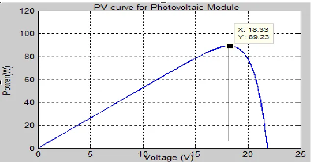
The most commonly applied hill-climbing MPPT techniques are the P&O algorithm and INC [9],[10]. The incremental conductance (INC) algorithm [11],[12] is based on the fact that the power–voltage curve of a PV generator at constant solar irradiance and cell temperature levels has normally only one MPP .At this MPP point, the derivative of the power with respect to the voltage equals zero as in Fig.2.
The INC algorithm increases the reference voltage (or decreases the duty ratio) if the operating point is LHS of the MPP otherwise decreases the reference voltage (or increases the duty ratio). A third condition in this algorithm is included [12] to keep the control parameter constant when ΔIPV/ΔVPV= IPV/VPV (i.e ΔPPV/ΔVPV=0. A partially
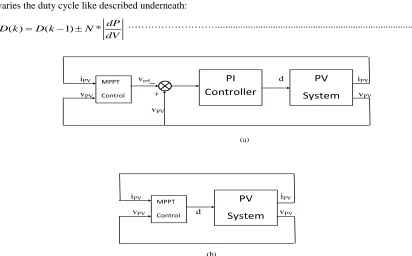
variable step size scheme has been used in [11] but this increases the complexity and cost of the algorithm. The principle of this InC algorithm is described [13].Two methods are utilized to implement the INC algorithm. Initial, orientation voltage perturbation during which a position significance for the PV group yield voltage be used like the organize factor here combination by a PI controller near regulate the duty ratio of the MPPT converter. Subsequent, through duty ratio perturbation [12] here which the duty ratio of the converter be used straightforwardly like the organize factor.Fig.3 shows block diagrams for these two realization techniques.
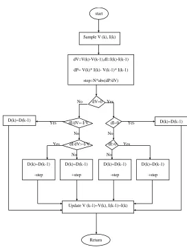
In this paper, an adaptive step size algorithm be applied designed for the INC MPPT technique to discover a easy and efficient mode of civilizing tracking exactness as fine as tracking dynamics. The flowchart of the customized variable step size INC MPPT algorithm is shown in Fig. 4, where the converter duty cycle iteration step size is by design tuned via by the PV yield to manage the duty cycle. V (k) and I(k) are the PV array output voltage and current at time k and d(k) is the duty ratio and vary of duty cycle is the step size correspondingly. The adaptive step size varies the duty cycle like described underneath:
( ) ( 1) * dP
D k D k N
dV
………... (1)
iPV vref d iPV
vPV vPV vPV
(a)
iPV iPV
vPV d vPV
(b)
MPPT
Control
PI Controller
PV
System
MPPT
Control
PV
System
Figure 3. Block diagrams of INC MPPT algorithms implementation techniques; (a) reference
No dV=0 Yes
Yes dI/dV=-I/V dI=0 Yes No No
Yes dI/dV>-I/V dI>0 Yes No No
Sample V (k), I(k) start
dV=V(k)-V(k-1),dI=I(k)-I(k-1) dP= V(k)* I(k)- V(k-1)* I(k-1)
step=N*abs(dP/dV)
D(k)=D(k-1) D(k)=D(k-1)
D(k)=D(k-1) -step
D(k)=D(k-1) +step
D(k)=D(k-1) -step
D(k)=D(k-1) +step
Update V (k-1)=V(k), I(k-1)=I(k)
Return
Figure 4. Flowchart of the variable step size INC MPPT algorithm.
where coefficient N is the scaling part which is tuned by the intend instance to regulate the step size. As revealed in Fig.4, the revise regulation for duty cycle can be obtained like follows:
P(k)-P(k-1) D(k)=D(k-1)±N*
V(k)-V(k-1)
……….……… (2)
Physical tuning of factor N is dreary also the obtained best outcome can be suitable merely for a certain scheme with working circumstance [14]. The steady-state value instead of lively value in the establish method [14] of the derivative of PV array yield power to voltage can be evaluated in the fixed step size process with ΔDmax, which will be selected like the higher limiter while the variable step size INC MPPT method. It is identified that |dP|/|dV |
is nearly by its lowest value about the PV MPP. To ensure the junction of the MPPT revise law, the variable step rule have to obey the subsequent:
max
max
*
fixedstep D dP
N D
dV
where |(dP/dV )|fixed step=ΔDmax is the |dP|/|dV | at fixed step size operation of ΔDmax. The scaling part can so be obtained as,
max/
fixedstep D dP
N D
dV
……….……….…………(4)
If (4) cannot be fulfilled, the variable step size INC MPPT will be operational by a set step size of the formerly locate higher limiter ΔDmax. Bigger N exhibits a relatively quicker response than a lesser N. The step size will turn
into small as dP/dV becomes tiny about the MPP.
IV IGBT BASED 3 LEVEL VOLTAGE SOURCE INVERTER DESIGN
The field of voltage source converter (VSC)-based multi terminal dc (MTDC) grids simulation includes short-circuit calculation [15], protection and control [16] that has experienced an outstanding evolution over the last years. Such popularity is mainly due to two reasons: appropriateness of the MTDC grids for the integration of offshore wind / solar farms and possibility of interconnecting several (more than two) ac networks with even non identical frequencies [17]. The first stage is called the input-side dc/dc converter for PVs. The second stage is called the grid-side converter, and is typically a dc/ac inverter for most systems. Both stages are described in upcoming section.
4.1 DC Voltage Control
The DC voltage control, lively power control, and power allocation be crucial equipped tasks in these grids in sort to agreement the suitable concert of the grid. An external voltage control loop is used to regulate the dc-bus voltage of the inverter. It determines the amplitude of the current to be injected to the grid such that the power balance between the first-stage and second-stage is satisfied. Here a conventional dc-bus voltage control method, a extremely small bandwidth PI controller is generally used to control the dc-bus voltage. The error signal processed by the PI controller is between the squares of the reference voltage and the dc-bus voltage. In this paper a three stage bridge inverter is used like a three stage power converter so as to consist of one, two or three arms of power switching strategy.
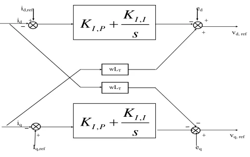
4.2. The Inner Current Controller
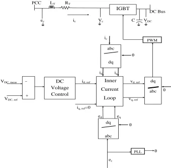
The most frequently used control approach for the VSC stations is based on the vector control [18]. In this approach, the ac currents and voltages of the converter station (at the PCC) are changed into the revolving direct–quadrature (d−q) orientation surround, coordinated by the ac grid voltage with way of a phase-locked loop (PLL). The common design of the vector control at a VSC-HVDC station is illustrated in Fig. 5. The dc voltage regulator in Fig. 5 is accountable for generating the reference currents (idref and iqref ) for the inner current controller (ICC), which
c c c T c T
di e v R i L
dt
……….………..………… (5)
where ic be the current flowing as of the ac grid toward the converter, with RT and LT correspond to the whole
resistance and inductance installed among the PCC and the converter. Next, with applying the d−q conversion, (6) can be uttered in the d−q orientation surround with
d
d d T d T T q
di
e v R i L wL i
dt
………... (6)
q
q q T q T T q
di
e v R i L wL i
dt
………..…….. (7)
where ω is the angular occurrence of the ac voltage on the PCC. The orientation voltages (vd,ref and vq,ref ), produced
through ICC, be next changed reverse into the abc orientation surround and used to produce the switching gesture of the converter.The alteration of the d-axis current (id) allows directing the dc voltage in the allowable restrictions.
PCC LT RT
DC Bus
ec ic Vc C VDC
ic
θ
id iq
VDC, meas id, ref vd, ref
θ
VDC, ref vq, ref iq, ref=0
ed eq θ θ ec _ DC Voltage Control Inner Current Loop dq abc PLL abc dq dq abc PWM IGBT
id,ref ed
id
vd, ref
iq
vq, ref Iq,ref eq
, , I I I P
K
K
s
, , I I I PK
K
s
wLT wLTFigure 6. The structure of ICC
V STANDALONE SYSTEMS
In rising countries, where rural electrification is emergent, the applications of photovoltaic (PV) systems be essential. Extending power lines to rural areas is frequently not so far cheap [20] therefore stand-alone photovoltaic systems be one of the inexpensive option in such isolated areas which have no admittance to a utility grid. These systems are providing trustworthy power for commercial, stand-alone, facility power, illumination, safety lighting, transportation etc. [19].In these PV stand-alone systems to take out the utmost power of the PV array, a series link is through in among dc–dc converter, PV array and the load or the energy storage constituent [21]. The process of the projected scheme is simulated by the execution on SIMULINK/MATLAB model, which is revealed in Fig. 7. The solar radiation and other meteorological parameters have been taken from the Solar Radiation Data Handbook [22]. The various parameters that have been used in this design are the PV module reference efficiency ηr= 15%,
reference solar cell temperature Tr = 25
◦
shows the waveform of current, voltage and power with PI Controller. There is greater oscillation in current, voltage and power without PI Controller as compared to with PI Controller as shown.
Figure 7. Simulink diagram of PV array connection with Standalone System
Figure 8. Solar Irradiance applied to the system
Figure 11. Output power without PI Controller
Figure 12. Output current with PI Controller
Figure 13. Output voltage with PI Controller
Figure 14. Output power with PI Controller
VI GRID CONNECTED PHOTOVOLTAIC SOLAR POWER SYSTEMS
In stand-alone situations, PVs are the mainly fiscal solutions to offer the requisite power. Likewise, with the growth of PV technologies, applications of PVs in grid-connected situations have developed quickly, signifying that PVs are especially striking to create environmentally caring electrical energy for diversified purposes [24]–[26]. Grid-connected PV schemes have two stages in conditions of control loops. The internal loop is a pulse width modulation (PWM) loop to convene the necessities of the waveform and stage. The external loop determines the yield power of the inverter according to the MPP of PV panels. [27]. Initial phase is a dc/dc converter by MPPT control and the additional is a dc/ac inverter. When the working spot of PV panels moves from MPP to its left area, the yield power will reduce on the similar instant, which will reason the dc-link voltage to fall down lastly. To pass up a dc-link voltage fall down incident in the PV grid-connected system, a competent MPPT control among an adaptive step technique is functional in segment of this editorial. The alteration of this technique focuses on the closed-loop control of power that is able to complete the obligation of high competence and high constancy.
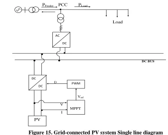
6.1 Structure of Grid-Connected Power System
Variations of load require be compensated through the major grid since the cause yield be keeping up to orientation power. The Grid-Connected PV scheme consists of a PV supply by the major grid linking to loads at the PCC like revealed in Fig.15.The photovoltaic [28], [29] are nonlinear voltage sources connected to dc–dc converters which are coupled at the dc side of a dc/ac inverter. In this paper boost converter is used as a dc–dc converters. The gate signal for the IGBT can be obtained by comparing the saw tooth waveform with the control voltage [30]. The PWM generates a gate signal to control the boost converter and, thus, maximum power is tracked and delivered to the ac side via a dc/ac inverter.
The complete simulink diagram of grid connected PV system is shown in Fig.16.It contains several blocks. The first block is of solar irradiance, here we have given step input of 1kW from t=0 to t=1sec and after that input is increased to 1.2kW from 1sec to 5sec (refer Fig. 8 from section 5).The other input for solar irradiance which can be given are constant type or ramp type. The another block is of PV array model it is described in previous sections (refer Fig 1(a) from section 2). After this PV array a capacitor C1 is attached it is about 100µF.It is used to reduce
the ripples in the voltage generated at PV array output. After C1 the action of ripples minimization the DC-DC boost
converter is designed block model is connected to increase the voltage obtained from PV array. The inductor L1 of
value 100 mH is attached after the capacitor C1. The boost converter has switching diode having on resistance value
(Ron) of 0.1 milliohm. Another switching device of boost converter is IGBT and its ON resistance is 0.001Ω. The
switching gate pulse for this IGBT is provided by incremental conductance algorithm (refer to section 3).
PFeeder PCC PLoad
Load
DC BUS
D
Vref
V I
PWM AC
DC
DC
DC
MPPT
PV
Figure 16. The simulink diagram of three phase grid connected photovoltaic system
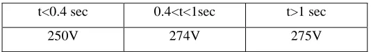
The simulink diagram of three phase grid is shown in Fig. 17. Three phase output is taken in such a way that PV array add on power to grid and fulfill the power demand of three phase load. The three phase load is star and, its nominal phase to phase rms voltage is 25kV and nominal frequency is 50Hz. The active power of three phase load is 10kW while inductive reactive power and capacitive reactive power of 100 VAR each. Fig.18 displays the dc output voltage of PV array prior to boosting operation. It can be observed that for t<0.4 sec, MPPT controller is not working. At this moment the PV array dc output voltage is 250V, at t>0.4 sec as the MPPT controller start working the voltage output starts rising & reaches a value of 274V with steady state at 0.44sec and it remains constant upto t<1 sec. At t>1sec the irradiance is changed from1000W/m2 to 1200 W/m2. Due to this a transient can be observed in the voltage with a instant and small time duration dip of 130V, because for t<1 sec the dc voltage was 274V and after t>1 sec it is 140V. But the MPPT controller retraces the voltage to 275V at t=1.06 sec with a stable state. The table 2 shows the variation of dc output voltage of PV array w.r.t. time.
Table 2
Variation of DC Output Voltage of PV Array
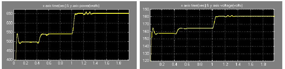
Fig. 19 displays the PV array power output w.r.t. time. It is obtained on running over simulink model for simulation time of 2 sec. It can be observed that the PV array output power is 96kW prior to initializing mppt operation. As the mppt starts working the output power increased to a value of 100kW within t=0.4sec to 0.42sec. As the irradiance is increased to t>1sec, power is enhanced to 122kW, hence the surplus power will be transferred to the grid side along with the compensation of power requirement of the load. The variation of power at the load end & of the PV array w.r.t. time is shown in table 3.
Table 3
Variation of Load & PV Array Power
Power t<0.4 sec 0.4<t<1sec t>1 sec
Load 78kW 81kW 100kW
PV Array 96kW 100kW 122kW
Figure 18. Output DC voltage of PV Array Figure 19. Output power of PV Array
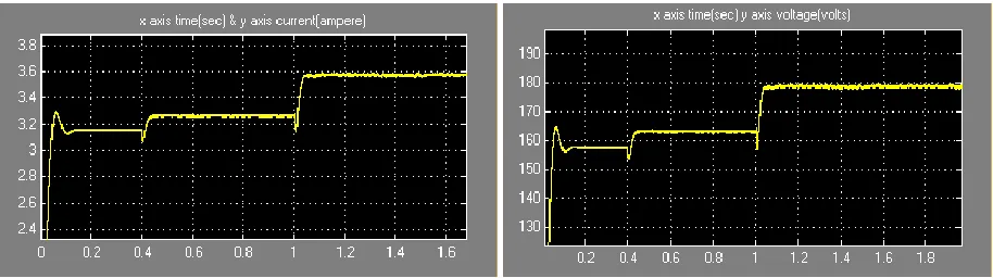
Fig. 20 shows the voltage & current obtained at the load end. Since the rated voltage of grid is 120kV that has been step down to 25kV prior to the connection with feeder hence in the Fig. 20 the voltage is 22kV. In the three phase current value, a small rise in current value after t>1 sec. The current rises from 3.5A to 4A. It is due to increase of irradiance. The current is increased but there is no change of the voltage at the load end after t=1 sec.
t<0.4 sec 0.4<t<1sec t>1 sec
Figure 20. Output three phase voltage and current of Grid
Figure 21. Output power of Grid
VII CONCLUSION
This paper contributes as a good guide for choosing which algorithm should be implemented for both standalone and grid connected application. In this paper, the conventional PWM method has been proposed for a three-phase boost-type grid-connected inverter. With the proposed incremental conductance method, the control circuit is simple and stable, and the overall system has a fast dynamic response. This cost-effective MPPT function can be integrated with the VSC with acceptable precision. Simulations have been performed with a 100-kW grid prototype connected to inverter to verify the performance of the proposed methods.
REFERENCES
[1] C. Wolfsegger and J. Stierstorfer, Solar Generation IV: Solar Electricity for Over One Billion People and Two Million Jobs by 2020. Amsterdam,The Netherlands: Greenpeace, 2007, EPIA.
[2] J. T. Stauth, M. D. Seeman, and K. Kesarwani, “Resonant switched capacitor converters for sub-module distributed photovoltaic power management,” IEEE Trans. on Power Elect., vol. 28, no. 3, 2013, pp. 1189- 1198.
[3] P. Sharma, P. K. Peter, and V. Agarwal, “Exact maximum power point tracking of partially shaded PV strings based on current equalization concept,” 38th IEEE photovoltaic Specialists Conference , 2012, pp.001411 - 001416.
[5] L. Shengyong, Z. Xing, G. Haibin, and X. Jun, “Multiport dc/dc converter for stand-alone photovoltaic lighting system with battery storage,” International Conference on Electrical and Control Engineering (ICECE), 2010, pp. 3894 - 3897.
[6] C. Zhao, S. D. Round, and J.W. Kolar, “An isolated three-port bidirectional dc-dc converter with decoupled power flow management,” IEEEtrans. on power elect. , vol. 23, no. 5, pp. 2443-2453, September 2008.
[7] G. R.Walker and P. C. Sernia, “Cascaded DC-DC converter connection of photovoltaic modules,” IEEE Trans. Power Electron., vol. 19, no. 4, pp. 1130–1139, Jul. 2004.
[8] E. Matagne, R. Chenni, and R. El Bachtiri, “A photovoltaic cell model based on nominal data only,” in Proc. Int. Conf. Power Eng., Energy Elect. Drives, POWERENG, 2007, pp. 562–565..
[9] M. A. Elgendy, B. Zahawi, and D. J. Atkinson, “Assessment of perturb and observe MPPT algorithm implementation techniques for PV pumping applications,” IEEE Trans. Sustain. Energy, vol. 3, no. 1, pp. 21– 33, Jan. 2012.
[10] Mohammed A. Elgendy, Bashar Zahawi, and David J. Atkinson, “Assessment of the Incremental Conductance Maximum Power Point Tracking Algorithm,” IEEE TRANSACTIONS ON SUSTAINABLE ENERGY, VOL. 4, NO. 1, pp. 681–689, Jan. 2013.
[11] Q. Mei, M. Shan, L. Liu, and J. M. Guerrero, “A novel improved variable step-size incremental-resistance MPPT method for PV systems,” IEEE Trans. Ind. Electron., vol. 58, no. 6, pp. 2427–2434, Jun. 2011.
[12] A. Safari and S. Mekhilef, “Simulation and hardware implementation of incremental conductance MPPT with direct control method using cuk converter,” IEEE Trans. Ind. Electron., vol. 58, no. 4, pp. 1154–1161, Apr. 2011.
[13] W. Ping, D. Hui, D. Changyu, and Q. Shengbiao, “An improved MPPT algorithm based on traditional incremental conductance method,” in Proc. 4th Int. Conf. Power Electron. Syst. Appl., 2011, pp. 1–4.
[14] A. Pandey, N. Dasgupta, and A. K. Mukerjee, “Design issues in implementing MPPT for improved tracking and dynamic performance,” in Proc. IEEE IECON, 2006, pp. 4387–4391.
[15] J. Yang, J. E. Fletcher, and J. O‟Reilly, “Short-circuit and ground fault analyses and location in VSC-based DC network cables,” IEEE Trans. Ind. Electron., vol. 59, no. 10, pp. 3827–3837, Oct. 2012.
[16] M. Han, L. Xiong, and L. Wan, “Power-synchronization loop for vector current control of VSC-HVDC connected to weak system,” in Proc. IEEE POWERCON, Oct./Nov. 2012, pp. 1–5.
[17] Y. Fu, Y. Wang, Y. Luo, H. Li, and X. Zhang, “Interconnection of wind farms with grid using a MTDC network,” in Proc. 38th Annu. IEEE IECON, Oct. 2012, pp. 1031–1036.
[19] V. Salas, M. J. Manzanas, A. Lazaro , A. Barrado, and J. Pierik, “The Control Strategies for Photovoltaic
Regulators Applied to Stand-alone Systems,” IEEE.,2002, pp. 3274–3279.
[20] Mohan Kolhe, “Techno-Economic Optimum Sizing of a Stand-Alone Solar Photovoltaic System,” IEEE Transactions on Energy Conversion, vol. 24, no. 2, pp. 511–519.
[21] Roger Gules, Juliano De Pellegrin Pacheco , Hélio Leães Hey andJohninson Imhoff “A Maximum Power Point Tracking System With Parallel Connection for PV Stand-Alone Applications,” IEEE Transactions on Industrial Electronics, vol. 55, no. 7,, pp. 2674–2683.
[22] A. Mani, Hand Book of Solar Radiation Data for India, 1980. New Delhi, India: Allied Publishers Private Limited, 1981.
[23] S. G. Tesfahunegn, O. Ulleberg, T.M. Undeland and P.J.S. Vie, “A Simplified battery charge controller for safety and increased utilization in standalone PV applications” . IEEE, 2011,pp. 137-144.
[24] J. C. Schaefer, “Review of photovoltaic power plant performance and economics,” IEEE Trans. Energy Convers., vol. 5, no. 2, pp. 232–238, Jun. 1990.
[25] Y. Chen and K. M. Smedley, “A cost-effective single-stage inverter with maximum power point tracking,” IEEE Trans. Power Electron., vol. 5, no. 19, pp. 1289–1294, Sep. 2004.
[26] E. V. Solodovnik, S. Liu, and R. A. Dougal, “Power controller design for maximum power tracking in solar installations,” IEEE Trans. Power Electron., vol. 19, no. 5, pp. 1295–1304, Sep. 2004.
[27] A. Lohner, T. Meyer, and A. Nagel, “A new panels-integratable inverter concept for grid-connected photovoltaic systems,” in Proc. IEEE Int. Symp. Ind. Electron., Warsaw, Poland, vol. 2, Jun. 17–20, 1996, pp. 827– 831.
[28] W. Xiao, W. Dunford, and A. Capel, “A novel modeling method for photovoltaic cells,” in Proc. IEEE 35th Annu. Power Electronics Specialists Conf., Jun. 2004, vol. 3, pp. 1950–1956.
[29] D. Sera, R. Teodorescu, and P. Rodriguez, “PV panel model based on datasheet values,” in Proc. IEEE Int. Symp. Industrial Electronics, Jun. 4–7, 2007, pp. 2392–2396.