Human Movement Patterns, Mobility Models and Their Impacts on Wireless Applications.

ABSTRACT

HONG, SEONGIK. Human Movement Patterns, Mobility Models and Their Impacts on Wireless Applications. (Under the direction of Dr. Injong Rhee.)

Simulating human mobility is important in most areas that rely on human movements such as the performance study of mobile networks, disease outbreak control, city planning, etc. To test these applications, deploying a real testbed for a target scenario and running experiments would be the best solution but such experiments are extremely difficult. Thus to have a realistic mobility model and to run simulations with that model is invaluable. Numerous mobility models have been proposed until now but it is still questionable whether they are “realistic” enough to reflect human movement patterns. Since a mobility model is most useful when it is able to reproduce the mobility patterns realistically in any possible environments, defining “realism” and reproducing it is a key factor in mobility modeling. In this dissertation, we define the “real” human movement patterns as the heavy-tail flights and inter-contact times (ICT) which is defined to be the time duration until two mobile nodes meet again after meeting previously. These are important factors to determine the performance of human related applications since they govern the meeting probabilities among users.

In this dissertation, we show that those features are key factors to reproduce heavy-tail flight and ICT distributions that match the distributions observed from empirical data sets. Based on these observations, we propose a mobility model, called Spatio-TEmPoral model (STEP), that contains all the properties mentioned above. With this model, we could generate synthetic heavy-tail flights and ICTs that exactly match those observed from empirical data sets.

c

⃝Copyright 2010 by Seongik Hong

Human Movement Patterns, Mobility Models and Their Impacts on Wireless Applications

by Seongik Hong

A dissertation submitted to the Graduate Faculty of North Carolina State University

in partial fulfillment of the requirements for the Degree of

Doctor of Philosophy

Computer Science

Raleigh, North Carolina 2010

APPROVED BY:

Dr. George N. Rouskas Dr. Khaled Harfoush

Dr. Steffen Heber Dr. Injong Rhee

DEDICATION

To my wife

Yeo-oak Yun

BIOGRAPHY

ACKNOWLEDGEMENTS

I would like to thank all people who have helped and inspired me during my doctoral study. First of all, I would like to thank my advisor, Dr. Injong Rhee, for his constructive guidance and support during my doctoral research. We had a long journey of Wednesday meetings for almost 4 years even on Christmas day and New Year’s Day. I could get many valuable comments and inspiration from the meetings. It was very fortunate for me to practice essential logical writing skills that I should have learned in my school days under his guidance. Also, I am very grateful to the other committee members, Dr. George N. Rouskas, Dr. Khaled Harfoush and Dr. Steffen Heber for their valuable comments.

This research is supported by various funding sources including the Korea Research Foun-dation. I would like to thank them for their support.

TABLE OF CONTENTS

List of Tables . . . .viii

List of Figures . . . ix

Chapter 1 Introduction . . . 1

Chapter 2 Prior Work: Descriptions of Existing Models . . . 10

2.1 Random Models . . . 11

2.1.1 RWP . . . 12

2.1.2 RD . . . 12

2.1.3 BM . . . 12

2.1.4 MWP . . . 12

2.1.5 GM . . . 13

2.1.6 SR . . . 13

2.1.7 RPGM . . . 13

2.1.8 VT . . . 13

2.2 Geographic Models . . . 14

2.2.1 OM . . . 14

2.2.2 Manhattan/Freeway . . . 15

2.3 Hotspot Models . . . 16

2.3.1 Dartmouth . . . 16

2.3.2 Pragma . . . 17

2.3.3 CMM . . . 17

2.3.4 ORBIT . . . 18

2.3.5 TCM . . . 18

2.4 Social Models . . . 19

2.4.1 CM . . . 19

2.4.2 SIMPS . . . 19

Chapter 3 Motivations. . . 21

3.1 Data Sets . . . 22

3.1.1 Experiments using GPS Receivers . . . 22

3.1.2 External Data Sets . . . 25

3.2 Summary of Observations from the Empirical Data Sets . . . 30

3.2.1 Spatial Features . . . 30

3.2.2 Spatio-Temporal Features . . . 33

3.3 Limitations of Existing Models . . . 38

3.3.1 Spatial Limitations . . . 38

Chapter 4 Spatial Features of Human Movements, Part I: Individual Patterns 46

4.1 Overview . . . 47

4.2 Characteristics . . . 50

4.2.1 Characteristic function . . . 50

4.2.2 Stationarity . . . 52

4.2.3 Diffusivity . . . 53

4.3 Inter-Contact Times . . . 57

4.3.1 Infinite Space . . . 57

4.3.2 Finite Space . . . 62

4.3.3 ICT Fitting . . . 66

4.3.4 Characteristic Time . . . 68

4.4 Routing Performance . . . 76

4.5 Conclusion . . . 86

Chapter 5 Spatial Features of Human Movements, Part II: Aggregation Pat-terns . . . 87

5.1 Overview . . . 88

5.2 Fractal Waypoint Maps . . . 89

5.3 Individual Movement Patterns . . . 92

5.3.1 LATP . . . 92

5.3.2 Individual Walker Model . . . 96

5.4 Performance Evaluations . . . 98

5.4.1 Flights . . . 98

5.4.2 Inter-Contact Times and Link Durations . . . 104

5.4.3 Routing Performance . . . 107

5.5 Conclusion . . . 111

Chapter 6 Spatio-Temporal Features of Human Movements: Individual and Aggregation Patterns . . . .112

6.1 Overview . . . 113

6.2 Spatial Features . . . 115

6.2.1 Fractal Dimension . . . 115

6.2.2 Super-Hotspot . . . 117

6.2.3 Sub-Hotspot . . . 118

6.3 Temporal Features . . . 121

6.4 Spatio-Temporal Correlations . . . 127

6.5 STEP Mobility Model . . . 130

6.5.1 Hotspot Model . . . 130

6.5.2 Individual Walker Model . . . 132

6.6 Performance Evaluation . . . 136

6.6.1 Experimental Validation . . . 136

6.6.2 Parameter Sensitivity . . . 138

LIST OF TABLES

Table 3.1 Statistics of collected mobility traces from five sites. . . 23

Table 3.2 AIC values : Truncated Pareto distributions give the best fit for the mea-sured distributions. . . 24

Table 3.3 Existing routing models can be categorized into four groups. Typical mod-els in every category have been listed. None of the existing modmod-els have all the characteristics of human walks. ’ ?’ means that it is unclear from the model description. . . 36

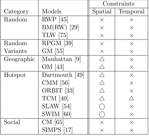
Table 3.4 Existing mobility models can be categorized by the constraints they de-scribe. None of the existing models can faithfully describe both spatial and temporal constraints. △means that the constraints proposed do not produce heavy-tail flight and ICT distributions. . . 39

Table 3.5 The results of Kullback-Leibler (KL) divergence tests : Each value repre-sents the KL divergence value between the distributions from the real data sets and each model. . . 43

Table 4.1 Diffusivity tendency by various parameters of TLW user mobility . . . 56

Table 4.2 The AIC and AW values for the ICT data from UCSD. . . 68

Table 4.3 The AIC and AW values for the ICT data from Dartmouth. . . 68

Table 4.4 The AIC and AW values for the ICT data from Infocom 2005. . . 71

Table 5.1 The result of the Akaike test for the maximum likelihood estimation of truncated Pareto distributions (denoted Par) and exponential distribution (denoted Exp) over flights (denoted FL) and ICTs extracted from syn-thetically generated traces from various models whose parameters are set based on real traces obtained from four different locations (KAIST, NCSU, NYC and Disney World). . . 100

Table 6.1 The results of Kullback-Leibler divergence tests : Compared with the re-sults in Table 3.5, STEP is at least 9.6 times and 2.4 times better than other models in reproducing the measured flight and ICT distributions, respectively. . . 138

LIST OF FIGURES

Figure 1.1 Lifecycles from a real data set and existing mobility models. . . 9

Figure 2.1 Sample traces from RWP and BM. . . 11

Figure 2.2 An example of node movement in the RPGM Model, providing two snap-shots at time T =t0 (left circle) and timeT =t0+ ∆t (right circle) [9]. . 14

Figure 2.3 An example of node movement in the OM Model. Shaded rectangles represent obstacles such as buildings. Dotted lines represent pathways between buildings. . . 15

Figure 2.4 The pathway graphs used in the Freeway and Manhattan models [9]. . . . 16

Figure 2.5 A view of the simulated mobility using Pragma. It shows a spatial dis-tribution of nodes in a bounded area. Each green point represents an individual mobile node, while red dots represent attractors that are lo-cated in the coordinates where individuals converge. . . 17

Figure 2.6 The Random ORBIT model. . . 18

Figure 2.7 An example of a social network. . . 19

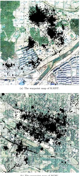
Figure 3.1 Waypoint maps from two campuses. . . 27

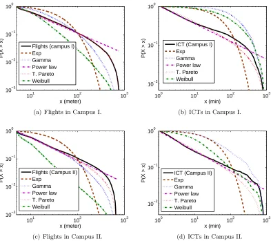
Figure 3.2 The CCDF of flights and ICTs measured from Campus I and II data sets. Various known distributions are fitted using MLE. . . 28

Figure 3.3 Hurst values and fractal dimensions of waypoints extracted from the ag-gregated traces of each campus. . . 29

Figure 3.4 It shows the self-similar nature of the dispersion of waypoints in the KAIST trace. At different scales, the dispersion of waypoints looks simi-larly bursty. . . 32

Figure 3.5 Lifecycles from a real data set and existing mobility models. . . 37

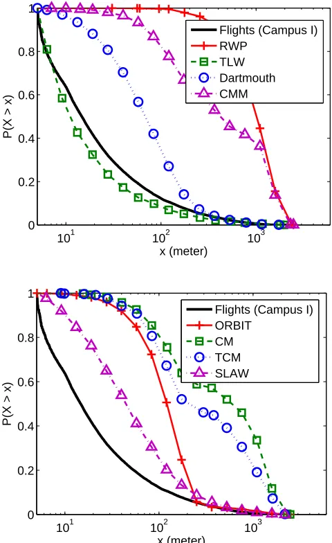
Figure 3.6 Flight distributions of synthetic traces from various models are compared with the measured flight distribution from the Campus I data set. Plots are divided into two for clarity. . . 44

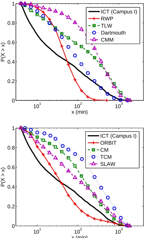
Figure 3.7 ICT distributions of synthetic traces from various models are compared with the measured ICT distribution from the Campus I data set. Plots are divided into two for clarity. . . 45

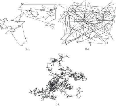
Figure 4.1 Sample traces of (a) TLW, (b) RWP and (c) BM . . . 48

Figure 4.2 Our TLW model can generate synthetic traces that match the flight and pause time distributions seen from real human walk traces. . . 50

Figure 4.3 The CDF of user displacement from their initial positions after the same amount of travel time. The RWP is most diffusive while the BM is least diffusive. The diffusion rates of Levy flights are in-between. The values in the parentheses represent Levy exponent for flight length. . . 54

Figure 4.4 The CCDF of ICT of Levy Walk in infinite space. . . 61

Figure 4.6 The CCDF of ICT collected from Dartmouth and UCSD. Various known distributions are fitted to the measured data distribution using the max-imum likelihood estimation technique. . . 69 Figure 4.7 The CCDF of ICT collected from Infocom 2005 and simulation result by

TLW. Various known distributions are fitted using MLE. TLW recreates the ICTD seen in the empirical data sets. . . 70 Figure 4.8 The ICT distributions of the TLW models. Levy walks recreate the

trun-cated Pareto ICT distributions seen in the empirical data sets. The num-bers in the figure represent the relaxation time from analyses. . . 75 Figure 4.9 A DTN routing delay according to the two hop relay algorithm. FCT and

RICT can be considered as the residual times of ICT. . . 77 Figure 4.10 The ICT and DTN delay distributions with single and multiple relays.

Results from both analysis and simulation are matching well. The values in parenthesis represent the number of relays. . . 80 Figure 4.11 The ICTDs of TLW (α=1.5, β=1) according to various amounts of

sim-ulated hours. The values in parenthesis represent delivery ratio. When the truncation of the ICTD comes from the insufficient duration of the simulation, the delivery ratio is less than one. . . 81 Figure 4.12 The ICT distributions of various mobility models. . . 83 Figure 4.13 The DTN delay distributions of various mobility models and normalized

99% quantile delay with multiple relays. The numbers in the parenthesis represent the actual delays in minutes at the 99% quantile of the distri-butions. . . 85 Figure 5.1 Hurst parameter estimation of waypoints registered in all KAIST traces. . 90 Figure 5.2 Hurst parameter values of waypoints in each site map. All show Hurst

values higher than 0.6 except NYC. . . 91 Figure 5.3 Measuring aggregated variance of waypoints aggregated from all walk

traces. We divide the area by non-overlappingdby dsquares, and count the number of waypoints registered in each square and then normalize the sampled count by the size of the unit square. We compute the normalized variance as we increase d. . . 91 Figure 5.4 Delaunay triangulation of waypoints extracted from one daily trace of

KAIST. In the inset, the CCDFs of the line lengths from the triangles and the flights from the same trace are plotted. The CCDF of flights and gaps match closely. . . 93 Figure 5.5 Delaunay triangulation is performed on all individual daily traces. The

line segment lengths in Delaunay triangles are aggregated and their CCDFs are plotted for different walkabout sites. The CCDF of flights obtained from the corresponding traces are also plotted for comparison. . . 94 Figure 5.6 For the GPS traces of 100 participants, we measure the percentage of

Figure 5.7 Flight distributions obtained from LATP for differentavalues performed on top of waypoints extracted from the KAIST traces and the percentage difference between the sum of flights generated from LATP and that of

flights from real traces . . . 97

Figure 5.8 Sample walk traces of various models. . . 102

Figure 5.9 Flight length distributions of synthetic traces from various models. . . 103

Figure 5.10 The ICT distributions of synthetic traces from various models . . . 105

Figure 5.11 The link duration distribution . . . 106

Figure 5.12 Average routing delays of various protocols under CMM. . . 109

Figure 5.13 Average routing delays of various protocols under Dartmouth, ORBIT and SLAW. . . 110

Figure 6.1 The relationship between the fractal dimensions (D) and the power-law slopes of corresponding gap distributions for sample fractal waypoint maps. The waypoint maps are generated by the Soneira-Peebles [80] model. . . 116

Figure 6.2 Hotspot size distributions. . . 117

Figure 6.3 Relationship between the average number of visitors (squares) and the number of waypoints (dots). . . 118

Figure 6.4 Area of individual movement observed from the Campus I data set. . . 119

Figure 6.5 Lifecycles from the Campus I data set and existing mobility models. . . . 124

Figure 6.6 Hotspot populations observed from the Campus I data set. Each square represents a hotspot. As the population increases, the square becomes darker. The incoming probabilities for hotspots 67 and 87 are shown. . . . 125

Figure 6.7 Hidden periodicity is discovered by eliminating the data collected during night time and weekends. . . 126

Figure 6.8 Various periodicity from hotspots in Campus I. . . 126

Figure 6.9 The number of primary periods for each hotspot is represented by black squares. As the number of primary periods increases, the square becomes brighter. . . 128

Figure 6.10 The STCs observed from the four data sets. Solid lines represent linear regression results. X-axis represents the distance from the super-hotspot to each hotspot. (a)(c)(e)(g) and (b)(d)(f)(h) show the number of visitors and number of primary periods, respectively. . . 129

Figure 6.11 The primary period distributions. They follow exponential distributions. . 130

Figure 6.12 Relationship between the number of waypoints and the number of primary periods for hotspots. . . 131

Figure 6.13 Assigned (solid line) and measured (dotted line) lifecycles for the proposed model. . . 136

Figure 6.14 A synthetic waypoint map generated by STEP hotspot model under the Campus I environment. We useD=1.4. . . 137

Figure 6.15 Flight and ICT distributions generated by STEP under the Campus I environment. We use γ=5. . . 140

Chapter 1

Simulating realistic mobility patterns of mobile devices is important for the performance study of mobile networks because deploying a real testbed of mobile networks is extremely difficult, and even with such a testbed, conducting repeatable performance experiments using mobile devices is not trivial. As most mobile nodes or devices (cell phones, PDAs and cars) are carried or driven by people, people are a critical factor in simulating mobile networks. Therefore, emulating the realistic mobility patterns of humans can enhance the realism in simulation-based performance evaluation of human-driven mobile networks.

“If life was so entertaining that we did not need any rest with ubiquitous supply of necessities

and no responsibilities, the movement paths could be a true time-space random walk.” - T. Hagerstrand, Regional Science, vol. 24, no. 1, pp. 6-21, December 1970.

People’s movement is not random and typically governed by spatial and temporal con-straints. People purposely visit a certain place at a certain time often driven by responsibilities and necessities. Capturing these constraints statistically and applying them to express real-istic movements of humans in user-created virtual mobility environments for mobile network simulation is the main goal of our work.

to another at a given time.

Another key difficulty in mobility modeling is to define realism. When we say that a synthetically generated mobility traces are realistic, what do we mean by “realistic”? It is impossible to mimic the movement of people to every little detail. Instead, we focus on the statistical features that can significantly influence the performance of mobile networks. It is commonly accepted that the distributions of inter-contact times (ICT) [17,22,25,38,47,54,65,75] and flights [54, 75] are the most influential characteristics of mobility traces determining the performance of mobile networks. ICT is the time duration until a node meets another node after meeting that node previously where meeting (or contact) is defined by being in a radio range. A flight is the Euclidian distance between two waypoints visited consecutively in time by the same person. A waypoint is a geographical location where a person pauses his or her movement (a more general notion of waypoint may include the location where people change movement directions; in this dissertation, we take a more simplified notion of waypoint).

The performance of mobile networks such as DTN undoubtedly depends on contact prob-ability. Mobile nodes forward and deliver messages when two nodes are in a radio range for a sufficient amount of time. Therefore, contact probability determines the probability and latency of message deliveries. The ICT distribution governs the probability of contact as it measures the time for a node to meet another from its last meeting. Flight distributions also influence the meeting probability. It is shown in [75, 77] that mobility with many long flights such as Random WayPoint (RWP) [45] tends to have high meeting probability than the one with many short flights such as Brownian Motion (BM) [29]. Flight patterns also determine the diffusivity of node distributions which is defined to be the distance that a node travels from an origin as a function of elapsed time. Longer flights induce higher diffusivity. ICT and flight patterns together characterize the probability of the existence of routing paths [75].

areas of mobility that people tend to have [22, 47, 75]. But the heavy-tail tendencies in flight and ICT distributions have never been observed together from the same mobility traces, largely due to lack of mobility traces from which detailed statistics about both flights and ICTs can be extracted. Some traces collected using iMotes [25] are good only for ICT measurements as they measure contact history while others [75] are for flight measurements as they track the GPS location of individuals and the individuals are not tracked at the same time. Some traces are based on WiFi associations of people [37, 59] or cell-tower association of cell-phone users [34]. But these data have too low resolution in their data with a margin of errors being a few hundred or thousand meters. Furthermore, while the WiFi data do not have wide coverage areas, so mobility outside the covered area is not recorded, the cell-phone data is not available to the public any more.

It is an academic interest what type of ICT distributions a given heavy-tail flight pattern may induce. While there have been several recent theoretical studies on related topics [17, 22, 47, 54, 65, 75], it is still an unsolved problem. However, it is conjectured, and verified by simulation [38, 54, 75], that power-law flights induce power-law ICTs. What’s more, obtaining both flight and ICT distributions from the same trace has a lot of practical value since they can be used to verify a mobility model. It is easy to construct a model that matches one of the features, but not both. For instance, we can imagine a variant of the RWP model where a node randomly picks a next waypoint in a way that the distance from the current waypoint (i.e., flight) follows a given heavy-tail distribution. So as long as the input flight distribution is realistic, the generated flight distribution from the model is trivially realistic. But it cannot be verified whether the synthetically generated traces induce a realistic ICT distribution as well since there is no corresponding ICT data to the flight distribution which can be used for the verification.

(North Carolina State Fair). The participants walk most of the time in these sites and may also occasionally travel by bus, trolley, cars, or subway trains. The GPS receivers record their location information every 5 seconds within a three meter margin of error. Two of the data sets are collected at the same time over a period of one week so contact information among the volunteers as well as their location information is available in those sets. The participants were recruited from the students at NCSU and KAIST who take a computer-literacy class and they are from over 30 different departments in each campus. Our data analysis confirms that all the data traces from both experiments have heavy-tail flight and ICT distributions. This is the first empirical study confirming the existence of heavy-tail tendency in flight and ICT distributions in the same traces.

We then use the measured ICT and flight data from our experiments to verify whether existing models are capable of reproducing realistic flight and ICT distributions. We have tested 8 different mobility models and by varying various input parameters for the models, we tried to fit their ICT and flight distributions to the measured distributions. Unfortunately, none of these models can match the flight and ICT distributions observed from the real traces. Most of them do not have heavy-tail tendencies in flight or ICT distributions.

We study how we can express both heavy-tail flights and ICTs from the spatial viewpoint. From the analysis results of our GPS data sets, we found out that the waypoints that people generate have a fractal nature and people unconsciously visit relatively near waypoints first. We conjecture that those two properties are related each other and would be the causes of heavy-tail flights and ICTs. To study the mechanism more in detail, we develop a mobility model. In this model, we generate a fractal waypoint map first. Then we apply a heuristic algorithm called Least Action Trip Planning (LATP) that generates a daily trip over these waypoints minimizing the total traveling distance. In this way, we can recover heavy-tail tendencies in flight and ICT distributions. But, unfortunately, they do not match closely the observed distributions from the data sets.

models is essentially due to the poor representation of spatio-temporal correlations present in real human mobility. Especially, ICTs are governed by where and when people meet. The mobility of people has regularity in their daily visiting locations and times. Most of students have daily schedules (classes and meetings) governing their visiting locations and times. For instance, classrooms have a tendency of being populated around class times with regular ups and downs in populations. Cafeterias and restaurants have typical high populations around meal times, and shopping areas or student unions tend to have more constant flows of populations with many small ups and downs.

Fig. 1.1 (a) shows our measured data of the population changes over one day time of four hotspots in a campus. We say that the function of population over time in a hotspot is the daily lifecycle function (DLF) of the hotspot. The daily lifecycle shown in the figure is clearly changing over time. Fig. 1.1 (b) shows the DLFs of a hotspot in other models. They are essentially flat, showing no temporal variations at all. This is because most of the models do not explicitly model the times at which a node visits a certain location, but rather choose the times randomly. We also find from our traces as well as other existing traces that waypoints are clustered together forming hotspots of various sizes. The size of a hotspot is defined by the number of waypoints within that hotspot. We find that there always exists at least one super-hotspot whose size dominates the mean of the hotspot sizes. This pattern is manifested by the power-law distribution of hotspot sizes. This notion is different from the clustering effect caused by the self-similarity of waypoints. What’s more, we find that the size and DLF of a hotspot is strongly correlated with the location of the hotspot. More precisely, (1) the size of a hotspot is inversely proportional to the distance of that hotspot to the super-hotspot and (2) the number of dominating frequencies in the DLF of a hotspot is proportional to that distance. We define a dominating frequency in a DLF to be a frequency component present in the function whose co-efficient is larger than a predefined threshold.

Mobility. STEP first generates hotspots of waypoints in an input mobility area using a self-similar point generation technique called the Soneira-Peebles (SP) Model [80]. Then we assign a DLF to each hotspot whose dominating frequencies are set according to linear correlation functions extracted from real traces. STEP provides a set of linear correlation functions that a user of STEP can choose from. We then construct an individual walker algorithm, using that each node chooses a next waypoint to visit for a given time and location. The algorithm is based on a non-linear weight function that combines the LATP and a lifecycle-based decision making algorithm.

With simple manipulations of input parameters, we verify that STEP can easily generate a synthetic mobility trace whose statistical characteristics, in particular, flight and ICT dis-tributions, match those of the real mobility traces. STEP takes as input a small number of parameters including the size of mobility area, the number of mobile nodes, the fractal dimen-sion of waypoints (D), and two constantsα and γ related to its individual walker model. The fractal dimension determines the gathering patterns of waypoints and governs the power-law slope of the flight length distribution. STEP considers two parameters when choosing the next waypoint, the distance from the current waypoint and the lifecycle of the next waypoint. α is a parameter to determine the degree of choosing the nearest neighbor waypoint as the next destination. α governs the power-law tendency of the flight distribution. γ determines the weight of lifecycles over the distance factor. By combining three inputs, D, α and γ, we could faithfully reproduce the flight and ICT distributions.

In this dissertation, we investigate “real” human movement patterns observed from empirical data sets. Based on the data analysis results, we propose a mobility model, STEP. By comparing the flight and ICT distributions generated from our model with the observed distributions from empirical data sets, we could confirm that our model faithfully reproduces reality.

80 84 88 92 96 0

10 20 30

Time (hours)

number of visitors

(a) Lifecycles measured from our data set during one daytime pe-riod.

20 30 40 50 60

0 10 20 30

Time (hours)

number of visitors

SLAW CMM ORBIT TLW RWP CM TCM Dartmouth

(b) Lifecycles from existing models.

Chapter 2

Prior Work: Descriptions of Existing

(a) A sample trace of RWP (b) A sample trace of BM

Figure 2.1: Sample traces from RWP and BM.

Existing mobility models can be largely categorized into several groups: random and its variants, geographic, hotspot and social models. These models vary in their movement char-acteristics. In random and its variant mobility models, the mobile nodes move in a given area without restrictions. The destination, speed and direction are chosen randomly and indepen-dently of other nodes. In geographic models, the movements of mobile nodes are restricted by geographical obstacles such as buildings, streets or freeways. A hotspot is a region where a large number of users stay and spend a relatively larger fraction of time. Hotspot models describe the aggregation tendency of mobile users. Social mobility models are founded on social network theory. The models allow mobile nodes to be grouped together when they have social relationships among them. The group is mapped to a geographical space, with movements influenced by the strength of social ties.

2.1

Random Models

2.1.1 RWP

In RWP, a mobile node chooses a random destination (waypoint) in a simulation area and moves to the waypoint with a speed chosen from a uniform distribution. In each waypoint, the user pauses for a certain period of time selected from a uniform distribution. After the pause, the mobile node chooses a new waypoint and moves there and it continues the process iteratively.

2.1.2 RD

In RD, a mobile node chooses a random direction in which to travel, then travels to the border of the simulation area in that direction. Once the simulation boundary is reached, the user pauses for a specified time, and continues the process.

2.1.3 BM

BM is a model named after the Scottish botanist Robert Brown. He noticed that pollen grains suspended in water showed a movement pattern following a zigzag path. BM characterizes the diffusion of tiny particles with a mean free path (or flight) and a mean pause time between flights. A flight is defined to be a longest straight line trip from one location to another that a particle makes without a directional change or pause. Einstein [29] first showed that the probability that such a particle is at a distance r from the initial position after a time thas a Gaussian distribution and thus is proportional to √t, i.e., the width or standard deviation of a Gaussian distribution. The mean squared displacement (MSD), which is defined to be the variance of the probability distribution, is proportional tot. It is a manifestation of the central limit theorem (CLT) as the sum of flight lengths follows a Gaussian distribution. BM is defined in a continuous space domain and RW is the another name of BM in a discrete space.

2.1.4 MWP

considered as random variant models. They have small improvements from random models in describing either spatial grouping behaviors or temporal dependencies in the velocity of users. For example, the MWP model allows adjusting pause times and momentary velocity. The distribution used to pick the next waypoint may depend on the current location, thus it implements Markovian transition probabilities among waypoints.

2.1.5 GM

The GM model is a variant of the RWP model. All the movement patterns except velocity are same as those of RWP. In the GM model, the velocity of a mobile node is assumed to be correlated over time and modeled as a Gauss-Markov stochastic process. It prohibits unrealistic abrupt velocity changes.

2.1.6 SR

The SR model is similar to the RWP model but instead of the sharp turn and sudden acceleration or deceleration, it proposes to change the speed and direction of node movement incrementally and smoothly [9, 13]. Mobility of a node may be limited by the physical laws of acceleration and velocity. The current velocity of a mobile node may depend on its previous velocity. Thus the velocities of a mobile node at different time slots are correlated. So the models such as GM and SR are calledtemporal dependency models [9].

2.1.7 RPGM

In RPGM, mobile nodes form several groups each of which contains one leader. All the members of a group move along their leader. Fig. 2.2 shows how the nodes move with RPGM.

2.1.8 VT

Figure 2.2: An example of node movement in the RPGM Model, providing two snapshots at timeT =t0 (left circle) and time T =t0+ ∆t(right circle) [9].

randomly placed in the the simulation area and they are interconnected by virtual tracks. Groups move along the virtual tracks towards the stations. At switch stations, a group can be split into multiple groups heading toward different stations or multiple groups can be merged into a single group. In random models such as RWP, a mobile node moves independently of other nodes. Thus, these models do not capture the co-location pattern of human mobility. But using the RPGM and VT models, we can describe the property. Therefore we can call these models, group mobility models.

2.2

Geographic Models

2.2.1 OM

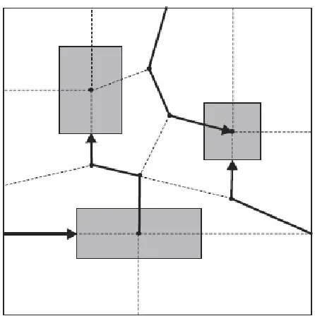
Figure 2.3: An example of node movement in the OM Model. Shaded rectangles represent obstacles such as buildings. Dotted lines represent pathways between buildings.

starting point to the selected destination for each node. Fig. 2.3 shows a sample trace with the OM model.

2.2.2 Manhattan/Freeway

Figure 2.4: The pathway graphs used in the Freeway and Manhattan models [9].

2.3

Hotspot Models

In representing social behaviors of humans, hotspot modeling is one of the most popular ways to represent collective behaviors. The Dartmouth [49], Pragma [16], Clustered Mobility Model (CMM) [56], and ORBIT [33] fall into this category.

2.3.1 Dartmouth

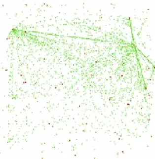
Figure 2.5: A view of the simulated mobility using Pragma. It shows a spatial distribution of nodes in a bounded area. Each green point represents an individual mobile node, while red dots represent attractors that are located in the coordinates where individuals converge.

2.3.2 Pragma

Pragma [16] is a realistic mobility model that is based on the behavioral characteristics of the individuals. It relies on a simple principle of dynamic network models namely the preferential attachment [12]. They translate the concept into the spatial distribution characteristic of mobile nodes using the concept of attractors. Attractors are landmarks to which humans move; they appear for a certain period of time, do not move, then disappear. Attractors describe centers of interest for people. Humans arrive, behave in cycles until their time is up, then depart. Fig. 2.5 shows a snapshot of nodes where they move with the Pragma model.

2.3.3 CMM

Figure 2.6: The Random ORBIT model.

2.3.4 ORBIT

ORBIT [33] randomly creates a specified number of hotspots within a given area and a subset of hotspots is assigned to each node. A node moves only among its assigned hotspots. For movements between and within hotspots, it is completely random. Fig. 2.6 shows a diagram how the mobile nodes move with the ORBIT model.

2.3.5 TCM

Figure 2.7: An example of a social network.

2.4

Social Models

Community Model (CM) [63,64] and Sociological Interaction Mobility for Population Simulation (SIMPS) [17] models fall into this category.

2.4.1 CM

CM [64] is a mobility model based on a social network theory. The CM model allows mobile nodes to be grouped together based on social relationships among individuals. The clustered group is then mapped to a topographical space. The movements of nodes are driven by the strength of the social relationships among them. In this model, the authors assumed that the strength of social ties can also be read as a measure of the likelihood of geographic co-location. They represent the social relationships in an Interaction matrix.

2.4.2 SIMPS

Chapter 3

3.1

Data Sets

To investigate common patterns of human movements, we decided to analyze human mobility traces. Currently, numerous empirical data sets are available [1] but most of them only provide contact information among participants collected using WiFi or Bluetooth devices [25, 41]. Those data sets do not provide precise location information of device holders since Bluetooth devices do not have any functionality to record their locations. From WiFi data sets, we can estimate a user’ s location from the location of the associated AP. It should incur a few hundred meters of location error [49].

To obtain human traces that contain fine-grained location information, we decided to collect new data sets using high quality GPS devices. GPS devices can record their locations with less than a few meters of error margin [2,3]. We have collected 7 data sets from our own experiments. We complement our data sets with 3 external data sets collected from Dartmouth College [37], UCSD [59] and the INFOCOM 2005 experiment [25].

3.1.1 Experiments using GPS Receivers

The 1st Experiment

Five sites are chosen for collecting human mobility traces from September 2006 to January 2008. These are two university campuses (NCSU in the US and KAIST in south Korea), New York city (NYC), Disney World (DW) and one State Fair (SF) all in the US. The total number of traces from these sites is 226 daily traces. Garmin GPS 60CSx handheld receivers were used for data collection. The receivers are WAAS (Wide Area Augmentation System) capable with a position accuracy of better than three meters 95 percent of the time, in North America [2]. Occasionally, track information has discontinuity when bearers move indoors where GPS signals cannot be received. The GPS receivers take readings of their current positions every 10 seconds and record them in a daily tracking log. The summary of daily traces is shown in Table 3.1.

Table 3.1: Statistics of collected mobility traces from five sites. Site (# of # of Duration (hour) Radius (km) participants) traces min avg max min avg max NCSU (20) 35 1.71 10.19 21.69 0.77 2.83 10.57 KAIST (32) 92 4.21 12.21 23.32 0.31 1.83 13.31 NYC (12) 39 1.23 8.44 22.66 0.42 6.60 17.74 DW (18) 41 2.17 8.99 14.28 0.25 3.60 16.79 SF (19) 19 1.48 2.56 3.45 0.17 0.51 0.86

in the computer science department. Every week, 2 or 3 randomly chosen students carried the GPS receivers for their daily regular activities. The KAIST traces are taken from 32 students who live in a campus dormitory. The New York city traces were obtained from 12 volunteers living in Manhattan or its vicinity. Their track logs contain relatively long distance trips. Their means of travel included cars, buses and walking. The Disney World traces were obtained from 18 volunteers who spent their Thanksgiving or Christmas holidays in Disney World, Florida, USA. The participants typically walked in the parks and occasionally rode trolleys. The state fair track logs were collected from 19 participants who visited North Carolina state fair which includes many street arcades, small street food stands and showcases. The event was very popular and attended by more than tens of thousands of people daily for two weeks. The site is completely outdoor and is the smallest among all the sites. Each participant in the state fair scenario spent less than three hours at the site.

The 2nd Experiment

Table 3.2: AIC values : Truncated Pareto distributions give the best fit for the measured distributions.

Campus I Campus II

flight ICT flight ICT

Exponential 188,878 219,061 193,569 27,243 Power law 169,012 170,917 166,946 19,305 Gamma 177,871 180,439 180,221 21,252 Truncated Pareto 167,755 166,892 165,965 18,891 Weibull 168,479 170,242 166,908 19,275

record only contact patterns hence, they do not provide spatial locations. WiFi data sets provide both spatial and contact information but their location information may contain a few hundred meters of errors.

To obtain mobility traces from which both detailed ICT and flight information can be extracted, we perform two measurement experiments. We have chosen two university campuses, KAIST and NCSU. We call both campuses as Campus I and II, respectively. Their maps and recorded waypoints are shown in Fig. 3.1. In each campus, we recruited about 100 student volunteers from over 30 different departments. All students from each campus are asked to carry the devices during the same week. Since the volunteers record their movements at the same time, we can extract very detailed flight and ICT distributions. Holux M-241 GPS loggers [3] are used for data collection with a position accuracy of better than five meters 95 percent of the time. The GPS receivers record their current positions at every five seconds.

Fig. 3.2 shows the CCDF (complementary cumulative density function) of flights and ICTs from each data set. We apply MLE to fit five known distributions, exponential, power-law, Gamma, truncated Pareto and Weibull distributions to the CCDF as done in [38]. The MLE of the truncated Pareto is performed over the x-axis range between the 1% and the 99% quantile of each distribution. We can observe visually that the truncated Pareto distribution fits best.

measured flight and ICT distributions are shown in Table 3.2. We can see that the truncated Pareto distribution gives the best fit. This result confirms that both heavy-tail flight and ICTs may be present from the same traces.

It has been known that the waypoints of humans can be modeled by self-similar points [54]. We also checked the similarity of the waypoints collected from both campuses. The self-similarity is generally quantified through the Hurst parameter which can be measured by two well-known methods, the Aggregate Variance (AV) and the R/S methods [82]. The sample data are said to be self-similar if the Hurst parameter is in between 0.5 and 1. Fig. 3.3(a) shows the Hurst parameter values obtained from both tests using the aggregated traces of each campus over one-dimensional (X and Y) and two-dimensional spaces. All values are over 0.68 and can be said to show strong self-similarity. We use the same method suggested in [54, 82] for the AV and R/S tests. Lee et al. [54] has shown that the Hurst parameter is a key factor to characterize the placement of waypoints.

Another common parameter to characterize the self-similarity is fractal dimension [58]. Fractal dimension is a quantity that represents how a fractal set fills a given space, as we zoom down to finer scales. A common characterization of a fractal set using this concept is provided by Minkowski dimension or box-counting dimension. We first imagine an evenly-spaced grid, and count how many boxes (grid squares) are needed to cover the set. Then as we make the grid finer, we see how this number changes. The numberN of boxes of sizeRrequired to cover a fractal set follows a power-law, N =N0·R−D, whereN0 is a constant and Drepresents the fractal dimension of the set. Fig. 3.3(b) shows the power-law tendencies in the number of boxes according to different box size. It shows the fractal dimensions are 1.4 and 1.5 for campus I and II, respectively.

3.1.2 External Data Sets

Dartmouth University [37], UCSD [59] and INFOCOM 2005 [25].

The Dartmouth trace data is one of the largest available sets of WiFi network traces collected since 2001. Dartmouth campus has over 190 buildings on 200 acres. Over 1,000 Cisco and Aruba APs are installed to completely cover the campus area. The traces collected contain data from nearly 10,000 users. Whenever clients authenticate, associate, roam, disassociate or de-authenticate with an AP, a syslog message is recorded, containing a timestamp in seconds, the client MAC address, the AP name and the event type. Since the Dartmouth trace data provides the locations of some APs, we can estimate the location of a client using the location of the associated AP. But it might incur a few hundred meters of location error [49].

The UCSD data set is collected from 275 freshmen PDA users for an 11 week period in 2002. The freshmen were the initial students in a new college on the university campus. Each PDA was equipped with a WiFi 802.11b network card. We can identify users according to their registered wireless card MAC addresses. But the mapping is anonymous. Since the UCSD trace data also provides the locations of APs, we can estimate the location of a user using the location of the associated AP. The UCSD data set is more exhaustive than the Dartmouth set, since it logs all reachable APs for each client at each time slot, while the Dartmouth data only logs the associated AP.

(a) The waypoint map of KAIST.

(b) The waypoint map of NCSU.

101 102 103 10−3 10−2 10−1 100 x (meter)

P(X > x)

Flights (campus I) Exp

Gamma Power law T. Pareto Weibull

(a) Flights in Campus I.

100 101 102 103

10−2 10−1 100

x (min)

P(X > x)

ICT (Campus I) Exp

Gamma Power law T. Pareto Weibull

(b) ICTs in Campus I.

101 102 103

10−3 10−2 10−1 100

x (meter)

P(X > x)

Flights (Campus II) Exp

Gamma Power law T. Pareto Weibull

(c) Flights in Campus II.

100 101 102 103

10−2 10−1 100

x (min)

P(X > x)

ICT (Campus II) Exp

Gamma Power law T. Pareto Weibull

(d) ICTs in Campus II.

I (AV) I (R/S) II (AV) II (R/S) 0.5 0.6 0.7 0.8 0.9 1 H X H Y H XY Sites Hurst Parameter

(95% and 99% Confidence Interval)

H_X H

Y

H

XY

H

X :1−D Stripe (X−axis)

H_Y :1−D Stripe (Y−axis) H

XY:2−D Grid

H

X

H_Y H

XY HX

H_Y

H_XY

(a) The Hurst parameter values (with 95% and 99% con-fidence interval) by the AV and R/S methods. Their val-ues indicate the self-similarity of waypoints. The X-axis represents the site and method used, e.g., ‘I (AV)’ rep-resents the Campus I and aggregated variance method.

100 101 102 103

100 101 102 103 104

r, box size

n(r), number of boxes

D = 1.4

D = 1.5

Campus I Campus II

(b) The fractal dimensions by the box-counting method.

3.2

Summary of Observations from the Empirical Data Sets

In this section, we show the characteristics of human movements extracted from empirical human traces. We have analyzed multiple data sets collected from various environments such as university campuses, a metropolitan area and theme parks. From all the results, we could confirm the same tendencies. Therefore, we can say that these properties do not rely on a specific condition and the following are general properties that are universally valid.

3.2.1 Spatial Features

Truncated power-law flights

Biologists [7, 71, 86] have found that the mobility patterns of foraging animals such as spider monkeys, albatrosses (seabirds) and jackals can be commonly described in what physicists have long called Levy Walks. The term Levy walks was first coined by Schlesinger et al. [78] to explain atypical particle diffusion not governed by Brownian motion (BM). BM characterizes the diffusion of tiny particles with a mean free path (or flight) and a mean pause time between flights. A flightis defined to be the longest straight line trip from one location to another that a particle makes without a directional change or pause. In Levy walks, flights follow a power law distribution.

In [74, 75], we have shown that statistical patterns of human walks observed within a radius of tens of kilometers. We use mobility track logs obtained from the first experiment 3.1.1.

From the data analysis of our traces, we find the followings:

• The mobility patterns of the participants in these outdoor settings have features congruent with those of Levy walks; their flight distributions and pause time distributions closely match truncated power-law distributions.

which may make the flight distribution appear like heavy-tailed or even short-tailed at times.

Our results are supported by [20, 34] which are conducted in different scales using tracking of bank notes and cellphone locations.

Several studies [49, 74, 75] also show that the pause time distributions of human walks show heavy-tail tendencies.

Heterogeneously bounded mobility areas

Gonzalez et al. [34] report that people mostly move only within their own confined areas of mobility and different people may have widely different mobility areas. They used two data sets to explore the mobility pattern of individuals. The first set (D1) consisted of the movement trajectories for 100,000 mobile phone users during a six-month period. Each time a user makes or receives a call or a message, the location of the routing cell tower was recorded. They reconstruct the users’ trajectories based on those data. To confirm that the obtained results were not affected by the irregular call pattern, they also studied a data set (D2) that captured the location of 206 mobile phone users. Their calls are recorded every two hours for an entire week. In both D1 and D2 data sets, the spatial resolution was determined by the density of over 100 mobile towers. The average coverage of the cell towers were approximately 3km2, and over 30% of the towers covered an area of 1km2 or less.

They found that the distribution of displacement of all users is well approximated by a truncated power law with cut-off values of 400km and 80km for each data sets D1 and D2, respectively.

(a) 4800m×1200m (b) 1200m×600m

(c) 300m×300m

Figure 3.4: It shows the self-similar nature of the dispersion of waypoints in the KAIST trace. At different scales, the dispersion of waypoints looks similarly bursty.

Fractal waypoints

The bursty dispersion of waypoints implies that people tend to swarm near a few popular locations and their popularity measured by the number of waypoints shows high burstiness: the popular locations tend to be very popular while most other areas are not.

can be split into parts, each of which is (at least approximately) a reduced-size copy of the whole” [57]. It is also called self-similarity.

Fractals are easily found in nature. Examples include coastlines, trees, ferns, mountain ranges, stellar matters, meteorites, moon craters and systems of blood vessels. It is very inter-esting the waypoints that humans make also have the fractal characteristics. The fractal nature of waypoints plays an important role in producing power-law flight length distributions. This fact will be explained in detail in chapters 5 and 6.

3.2.2 Spatio-Temporal Features

Truncated power-law inter-contact times

DTN provides a challenging environment in which communications between nodes are inter-mittent [31]. DTN does not assume that there exists connectivity between nodes at a certain point in time. When the nodes are disconnected, the packets are stored and forwarded through intermittent contacts established by the mobility of the nodes. In this type of networks, ICT is a key determinant of routing performance.

Many simulation and theoretical studies of DTN routing (e.g. [35, 77]) have long assumed that the ICT distribution (ICTD) of human walks follows an exponential distribution. Expo-nential distributions make mobility analysis tractable and the simulation results with popular mobility models [23] such as the RWP and RD models can easily produce exponentially decay-ing ICT distributions. But recently, empirical studies [25] show that this assumption is wrong especially in the context of human mobility: the ICTD of human walks contains a power law tendency. Under the assumption that the ICTD has a power law tail, the DTN routing delays approach infinite because of the presence of infinitely long inter-contact times.

tails imply that the delay of opportunistic routing algorithms should be finite in contrast to the infinite delay under the power law ICTD assumption.

We do not yet have mathematical models to describe the dichotomy of ICTD that are easy enough like exponential distributions for the performance analysis of DTN routing. To solve this problem, we analyze three empirical data sets of human ICT [38]. We observe from Maximum Likelihood Estimation (MLE) and Akaike test [50] results that the ICTD closely follows a truncated Pareto distribution. Truncated Pareto distributions have a truncation point that corresponds to the characteristic time in the ICTD. We show that the closed form expression of DTN routing delay can be induced from the ICTD model.

Spatio-Temporal Correlations

The mobility of people has regularity in their daily visiting locations and times. For example, most of students have daily schedules (classes and meetings) governing their visiting locations and times. Classrooms have a tendency of being populated around class times with regular ups and downs in populations, cafeterias and restaurants have typical high populations around meal times, and shopping areas or student unions tend to have more constant flows of populations with many small ups and downs.

Fig. 3.5 (a) shows our measure data of the population changes over one day time visiting four popular hotspots in a campus. The DLF shown in the figure is clearly changing over time. Fig. 3.5 (b) shows the DLF of a hotspot in other models. They are essentially flat, showing no temporal variations at all.

We find that the size and location a hotspot and the characteristics of its DLF are strongly correlated as follows.

• The size of a hotspot is inversely proportional to the distance of that hotspot to the super-hotspot.

Using these findings on the spatio-temporal correlations present in the human mobility traces, we construct the STEP mobility model. STEP and the spatio-temporal correlations will be explained in more detail in Chapter 6.

In summary, Table 3.3 shows how the existing models satisfy the characteristics of human movements mentioned above. F1 to F5 represent the followings.

• (F1) Truncated power-law fight lengths and pause-times • (F2) Heterogeneously bounded mobility areas

• (F3) Truncated power-law inter-contact times

• (F4) Fractal waypoints

Table 3.3: Existing routing models can be categorized into four groups. Typical models in every category have been listed. None of the existing models have all the characteristics of human walks. ’ ?’ means that it is unclear from the model description.

Features F1 F2 F3 F4 F5 Category Models

Random RWP [45] N N N N N

RD [15] N N N N N

BM(RW) [29] N N Y N N

Random MWP [42] N N N N N

Variants GM [55] N N N N N

SR [13] N N N N N

RPGM [39] N N ? N N

VT [87] N N ? N N

Geographic Freeway [8] N N ? N N

Manhattan [8] N N ? N N

OM [43] N N ? N N

Hotspot Dartmouth [49] N N N N N

Pragma [16] N N ? N ?

CMM [56] N N N N N

ORBIT [33] N Y N N N

TCM [40] N Y N N Y

Social CM [64] N N Y N N

80 84 88 92 96 0

10 20 30

Time (hours)

number of visitors

(a) Lifecycles measured from the Campus I data set during one daytime period.

20 30 40 50 60

0 10 20 30

Time (hours)

number of visitors

SLAW CMM ORBIT TLW RWP CM TCM Dartmouth

(b) Lifecycles from existing models.

3.3

Limitations of Existing Models

3.3.1 Spatial Limitations

Numerous mobility models have been proposed [9]. They can be categorized in several groups according to spatial and temporal constraints they represent as shown in Table 3.4. Spatial constraints are the constraints that a model explicitly imposes to control flight patterns. Tem-poral constraints are pertaining to ICT patterns. A mobility model provides an algorithm to choose the next waypoint from the current waypoint. This algorithm governs the spatial and temporal features of a mobility model. When the next waypoint are chosen without any con-straint, e.g., randomly chosen from a uniform distribution, we say that the model does not put any constraints on node movement.

In random and its variants models (e.g., [29, 45]), the nodes move in a simulation area without any restrictions so no spatial and temporal constraints are represented. Geographic and hotspot models (e.g., [9,43]) describe a type of spatial constraints that humans likely show. For example, the Manhattan model [9] uses a grid map and nodes move in horizontal or vertical direction on the map. Clustered Mobility Model (CMM) [56] uses the preferential attachment theory [11] to describe human gathering patterns.

Table 3.4: Existing mobility models can be categorized by the constraints they describe. None of the existing models can faithfully describe both spatial and temporal constraints. △means that the constraints proposed do not produce heavy-tail flight and ICT distributions.

Constraints Category Models Spatial Temporal

Random RWP [45] × ×

BM(RW) [29] × ×

TLW [75] × ×

Random RPGM [39] × ×

Variants GM [55] × ×

Geographic Manhattan [9] △ ×

OM [43] △ ×

Hotspot Dartmouth [49] △ ×

CMM [56] △ ×

ORBIT [33] △ ×

TCM [40] △ △

SLAW [54] ⃝ ×

SWIM [60] ⃝ ×

Social CM [65] × ×

SIMPS [17] × ×

(TCM) [40] models, after communities are determined, they are associated to a location in the simulation area with a uniform distribution. Other models that are not mentioned here such as [16, 17] also use similar random selection mechanisms. So the resulting flights are not heavy-tail. SLAW [54] is the only model that does not choose the next waypoint randomly using a uniform distribution. It shows that a self-similar placement of waypoints and the LATP algorithm which assigns more weight on the waypoints near to the current waypoint in choosing the next waypoint induce a power-law flight distribution.

is chosen randomly from a uniform distribution. Also it is not proven whether the temporal constraint of TCM enforces a heavy-tail ICT distribution. As shown above, numerous mobility models have been proposed but as far as we know none of the existing models can describe both spatial and temporal features of human movements.

3.3.2 Spatio-Temporal Limitations

In this section, we run mobility simulations using various mobility models to examine whether the exiting models can produce the flight and ICT distributions similar to the measured dis-tributions from our traces. We examine RWP [45], TLW [75], Dartmouth [49], CMM [56], ORBIT [33], CM [65], TCM [40] and SLAW [54]. We tested using both Campus I and II data sets. Both tests produce similar results. To save the space, we present only Campus I test.

Setup

For simulation of various models, we use the following setup. These parameters are common to all models. We fix the simulation areas to be approximately the same as the measurement site of Campus I which is 2km by 2km. We assume that the entire area is divided into a number of equal-sized square cells of 200m by 200m. The transmission range of each node is set to 50 meters as in [54, 75]. 70 nodes are simulated for 56 hours and the first 24 hours of simulation results are discarded to avoid transient effects. The speed of every user is set to 1 m/s for simplicity as in [54, 75]. We use the pause time distribution obtained from Campus I traces.

For other input parameters to each model, we run many experiments and find the values that match the measured flight and ICT distributions best. In CMM, clustering exponent, ce, determines the level of preferential attachment. When ce is equal to 0, nodes randomly

choose their next waypoints from the whole area with the uniform distribution. Asce increases,

the preferential attachment patterns become stronger so nodes tend to gather around in the biggest hotspot. We found thatce = 2 produces the best result. In CM, rewiring probability,

pr, determines the probability of interaction with the nodes in other communities. Initially,

each community has a group of nodes and each node in a community is connected to each other within the community by an edge. Withpr, each edge is broken and reconnected to a node in

the other communities. As we increasepr, the tails of the flight distribution become longer. pr

= 0.1 produce the best matching to the measured distributions. In SLAW, when the distance exponentαbecomes larger, then a node is more likely to choose the nearer unvisited waypoint. α = 4 produces the best matching heavy-tail tendencies to the given distributions. In TCM, pl is the probability to choose the local epoch. A node has two different modes of movement:

local and roaming epochs. In a local epoch, the mobility of the node is confined within its community. In a roaming epoch, the node is free to move in the whole simulation area. At the end of each epoch, the node chooses the next epoch to be local with probability pl. We set pl

= 0.75 to generate the best matching flight and ICT distributions.

Flight and ICT distributions

parameter can be obtained when the average KL distance becomes the minimum.

We conjecture that the discrepancies between the measured flight and ICT distributions and those from each model come from the random selection mechanism mentioned in Section 3.3.1. When the nodes choose their next waypoints from a uniform distribution, the probability to have relatively short flights (e.g., less than 100 m) becomes small. We can also confirm this from Fig. 3.6. For example, in the real traces the proportion of flights less than 100 m is about 0.8. But with the RWP model, the generated flights are larger than 100 m.

TLW and SLAW seem to match the measured flight distribution better than other models. In TLW, the next waypoint is selected in a way that the resulting flight distribution follows a given heavy-tail distribution. But TLW is a random model so it cannot describe interactions among mobile nodes, which means it does not have hotspots where people gather together. SLAW first generates a self-similar waypoint map and mobile nodes move along a subset of the waypoints using the LATP algorithm. In this way, SLAW could reproduce the heavy-tail tendency present in the measured flight distribution. But we have found that the flight distribution by SLAW shows only heavy-tail tendencies and it is not a good match to the measured distribution. In addition, we set the distance exponent α = 4 to obtain the best fit, which implies that nodes move mostly to the nearest waypoint. It is our common sense that people do not always move to the nearest location since most people have daily schedules governing their visiting locations.

Table 3.5: The results of Kullback-Leibler (KL) divergence tests : Each value represents the KL divergence value between the distributions from the real data sets and each model.

Campus I Campus II Flight ICT Flight ICT RWP 0.6300 0.2048 0.6389 0.2343 TLW 0.0125 0.0430 0.0221 0.0321 Dartmouth 0.0485 0.0161 0.0529 0.0421 CMM 0.3686 0.0505 0.3781 0.0655 ORBIT 0.1042 0.0148 0.1112 0.1019 CM 0.2639 0.0175 0.2347 0.0231 TCM 0.2124 0.0491 0.2245 0.0527 SLAW 0.0224 0.0171 0.0312 0.0192

We conjecture that the second cause of the discrepancy is the lack of descriptions on temporal human movement patterns. The flight distribution is governed by only the spatial movement patterns but the ICT distribution is also determined by temporal features of movements since contacts occur when people go to the same place at the same time. As we have shown in Table 3.4, none of the existing models faithfully describe the temporal features of movement patterns. As a summary, we perform the Kullback-Leibler (KL) divergence test [51] to quantify the closeness of the flight and ICT distributions generated by various mobility models to the mea-sured distributions. The model that gives the minimum KL value means the best fit for the measured distribution. The table also contains the simulation results obtained from Campus II environments. The parameters used are measured from the Campus II data set. Table 3.5 shows that TLW and SLAW show relatively better matching results than other models in reproducing the measured flight and ICT distributions.

101 102 103 0

0.2 0.4 0.6 0.8 1

x (meter)

P(X > x)

Flights (Campus I) RWP

TLW Dartmouth CMM

101 102 103

0 0.2 0.4 0.6 0.8 1

x (meter)

P(X > x)

Flights (Campus I) ORBIT

CM TCM SLAW

101 102 103 0

0.2 0.4 0.6 0.8 1

x (min)

P(X > x)

ICT (Campus I) RWP

TLW Dartmouth CMM

101 102 103

0 0.2 0.4 0.6 0.8 1

x (min)

P(X > x)

ICT (Campus I) ORBIT CM TCM SLAW

Chapter 4

Spatial Features of Human

Movements, Part I: Individual

4.1

Overview

In this chapter, we focus on the individual movement patterns, i.e., heavy-tail or truncated power-law flight and pause time distributions. To evaluate the impacts of those patterns, we propose a simple model, Truncated Levy Walk (TLW), that contains both properties. We eval-uate its characteristics such as ICTs and Delay Tolerant Network (DTN) routing performances. p(l) and ψ(t) represent flight and pause time probability density distributions in TLW,

respectively. Then their asymptotic behaviors can be expressed as follows [46].

p(l)∼ |l|−(1+α) (4.1)

ψ(t)∼t−(1+β),where t >0 (4.2)

αandβhave a value between 0 and 2. Whenα(orβ) is 2,p(l) (orψ(t)) becomes a Gaussian distribution. Whenα≥2, the model becomes BM due to the central limit theorem [79]. Flights and pause times cannot exceed certain values,fmax andpmax, respectively. Fig. 4.1 illustrates

sample traces of TLW, RWP and BM.

In TLW, a step is represented by four variables, flight length (l), direction (θ), flight time (∆tf), and pause time (∆tp). Our model selects flight lengths and pause times randomly from

their PDFsp(l) andψ(∆tp) which are Levy distributions with coefficientsαandβ, respectively.

The following defines a Levy distribution with a scale factor c and exponent α in terms of a fourier transformation,

fX(x) =

1 2π

∫ +∞

−∞ e

−itx−|ct|α

dt (4.3)

For α = 1, it reduces to a Cauchy distribution and for α = 2, a Gaussian with σ = √2c. Asymptotically, for α <2, fX(x) can be approximately by _|x|1+1 α. We allow c, α and β to be

(a) (b)

(c)

∆tf =kl1−ρ,0≤ρ ≤1 wherek and ρ are constants. In one extreme, whenρ is 0, flight times

are proportional to flight lengths and it models the constant velocity movement. In another extreme, when ρ is 1, flight times are constant and flight velocity is linearly proportional to flight lengths. In our measurement data, the relation is best fitted withk= 18.72 andρ= 0.79 when l <500m, and withk= 1.37 and ρ= 0.36 when l≥500m.

Based on the above model, we generate synthetic Levy-walk mobility tracks with truncation factors τl and τp for flights and pause times respectively in a confined area as follows. First,

the initial location of a walker is picked randomly from a uniform distribution in the area. At every step, an instance of tuple (l, θ,∆tf,∆tp) is generated randomly from their corresponding

distributions. If l and ∆tp are negative or l > τl or ∆tp > τp, then we discard the step and

regenerate another step. We repeat this process after the step time ∆tf + ∆tp. Until the end

of the simulation, we generate the tuples repeatedly.

Now we verify whether TLW can synthetically generate the statistical features we have observed in our traces. Figs. 4.2 (a) and (b) show statistical distributions of flights and pause-time matching each scenario (we do not show the matching of NCSU data as it is similar to that of KAIST). To produce these traces, we set the simulation area by the same size of each corresponding scenario. We then vary the values ofα and β to find synthetic traces that have similar flight length and pause-time distributions of each scenario. We do not add any geographical constraints other than the simulation area (i.e., we setτlto infinity) and any flight

that goes outside the area is abandoned and a new flight is generated. We set the truncation of pause time (τp) using the same values we obtained from the traces. Our synthetic traces show