History Reuse Architecture: Reuse of Historical Computations across Iterations of a Converging Algorithm.

(1)

ABSTRACT

PURI, SHANIL . History Reuse Architecture: Reuse of Historical Computations across Iterations of a Converging Algorithm. (Under the direction of Dr. Xipeng Shen .)

In this data explosion era, there are myriad programs that are executed repeatedly on large sets of data, consuming high amounts of energy and resources. Critical process reused on different data

sets will no doubt help reduce the time and computations.

This thesis explores how Computation Reuse can be implemented for augmenting the perfor-mance of some time consuming data analytics algorithms. Specifically, we developed a general

framework for efficiently finding similar datasets and effectively reusing history. We demonstrated

(2)

(3)

History Reuse Architecture: Reuse of Historical Computations across Iterations of a Converging Algorithm

by Shanil Puri

A thesis submitted to the Graduate Faculty of North Carolina State University

in partial fulfillment of the requirements for the Degree of

Master of Science

Computer Science

Raleigh, North Carolina

2016

APPROVED BY:

Dr. Frank Mueller Dr. Min Chi

(4)

DEDICATION

(5)

BIOGRAPHY

The author was born in the small town Sitapur in India. He attended Guru Gobind Singh Indraprastha University, Delhi where he obtanined his Bachelor’s in Information Technology from Maharaja

Surajmal Institute of Technology. After graduation he worked for a couple of years in a startup, being

one of the first members of the tech team and helped build it into a global barnd in the field of AB testing. He was admitted to NC State in the Fall of 2013 as a Master’s student to the Department

of Computer Science. He has worked under Dr. Xipeng Shen as a Research Assistant since August 2015 with research in the area of Algorithmic Optimization, which has culminated with this a new

methodology for the Initialization of converging algorithms with History Reuse, which has been

(6)

ACKNOWLEDGEMENTS

I would like to express my gratitude to my advisor Dr Xipeng Shen for the useful comments, remarks and engagement through the learning process of this master thesis. His constant guidance through

the process has been invaluable, be it teaching me the correct research methodology or discussing

with me solutions for problems. His constant guidance was imperative in the successful completion of this thesis.

I would also like to take this opportunity to thank Dr Frank Meuller for providing me help with all the hardware that I needed for experimentation and agreeing to serve on my thesis committee.

I would also like to thank Dr. Min Chi for serving on my thesis committee.

Last but not the least, I would like to thank my loved ones, who have supported me throughout entire process, both by keeping me harmonious and helping me putting pieces together. I will be

(7)

CONTENTS

List of Tables. . . vii

List of Figures. . . .viii

Chapter 1 INTRODUCTION . . . 1

Chapter 2 Motivation and Background . . . 4

2.1 Motivation . . . 4

2.2 Background and Related Work . . . 5

2.3 Important Terminology . . . 7

Chapter 3 Challenges . . . 9

3.1 Data Feature Abstraction . . . 9

3.2 Similarity Computation . . . 10

3.2.1 Non Uniform Scale . . . 10

3.2.2 Different Feature Sets: Feature Set Abstraction . . . 10

3.2.3 Rotated Data . . . 10

3.3 Efficient and effective comparison . . . 11

3.4 How to use the historical datasets . . . 11

Chapter 4 History Reuse Architecture . . . 12

4.1 Overview . . . 12

4.1.1 Feature Set Reduction And Normalization . . . 12

4.1.2 Similarity Metric Calculation . . . 13

4.1.3 History Storage Architecture . . . 13

4.1.4 Matcher and Selector . . . 14

4.2 Algorithm: HRu Architecture . . . 14

4.2.1 Principal Component Analysis (PCA) . . . 15

4.2.2 Histogram Generation . . . 15

4.2.3 Similarity Metric Computation . . . 17

4.2.4 Training Algorithm . . . 17

4.2.5 Computing Best Match for Current Data-set (Run Time) . . . 21

4.3 Discussion . . . 22

4.3.1 Computation on Real Data and Incorrect Screening algorithm: . . . 22

4.3.2 Custom CPP Implementation for Welch’s Test . . . 23

4.3.3 Random Sampling for Order comparison. . . 24

4.3.4 Use Of PCA Data for Welch’s Test and PCA data for centroid computation in Training Run: . . . 25

Chapter 5 Evaluations . . . 26

5.1 Methodology . . . 26

(8)

Chapter 6 Future Work . . . 40

Chapter 7 Conclusion. . . 42

(9)

LIST OF TABLES

Table 5.1 Selection Hit Rate K-Means History Reuse . . . 29 Table 5.2 Runtime comparison: K-Means, K-Means++and K-Means-HRU(*All times in

µS) . . . 35 Table 5.3 Median Iteration count comparison for K-Means, K-Means++and K-Means

(10)

LIST OF FIGURES

Figure 4.1 PCA Projection Example . . . 16

Figure 4.2 Feature Set Abstraction . . . 16

Figure 5.1 Hit-Rate (Road Network k=120) . . . 27

Figure 5.2 Hit-Rate (Caltec 101 for k=600) . . . 28

Figure 5.3 Best Match Selection Overhead (Maximum for Smallk) . . . 31

Figure 5.4 Best Match Selection Overhead (Minimum for Largek) . . . 32

Figure 5.5 Performance for various PCA Dimension Count(Caltec 101; K=600). Default PCA Dims: 3 . . . 33

Figure 5.6 Median Speed up, Small Data (k=240) . . . 34

Figure 5.7 Median Speed up, Large Data (k=600) . . . 36

Figure 5.8 Median Speed up, Small Data (k=240)(*K-HRu: K-Means-History Reuse; Kpp: K-Means++) . . . 38

(11)

CHAPTER

1 INTRODUCTION

In this data explosion era, there are myriad programs that are executed repeatedly on large sets of data, consuming high amounts of energy and resources. Critical process reused on different data

sets will no doubt help reduce the time and computations. In this work we will introduce a new

probabilistic model of measuring data similarities. Based on these data similarities we will show how critical computations may be reused across data sets, saving energy and improving performance.

Our work will introduce a general architecture for comparing two or more data sets and get a

probabilistic measure of similarity. We reason that if two data sets are similar, computation reuse from previous iteration of an algorithm for the similar data set will provide a good speed up in the

execution of the algorithm for the current data set. We first define the architecture to compute the

above-mentioned metric of similarity and then proceed to validate our above-mentioned stipulation for the K-Means and the SGD based SVM algorithms.

In these explorations, we found challenges in 4 aspects:data features, similarity definition, scalability,andreuse. Data features, is the description of data sets. Similarity definition (distance between two data sets) is the metric we use to describe similarity between data sets. Data feature and

distance definition are used together for reuse instance selection from a program specific database. The selection of history record is the most essential part of computation reuse.

(12)

CHAPTER 1. INTRODUCTION

based on data features, the problem becomes even more complex. Scalability issues are related with number of instances in database, size of the target data set, and dimension of data-set. Goal

of computation reuse is to save computation time and energy. In order to select a suitable history

record, some extra computation is inevitably introduced. The dilemma is the trade-off between the amount of computation reuse and the introduced overhead.

Reuse, thus is the process to decide what history information the program should reuse and how

to reuse the pre-computed information. In this study we introduce the concept of Historical Com-putation reuse. This is an Intuitive Idea whose exploration for the family of algorithms mentioned

above is spotted at best.

Computation Reuseis the process of deciding what history information the program should

reuse and how to best reuse the pre-computed information. While the idea is simple and intuitive

in nature, it promises big gains if correctly implemented with a wide variety of uses. In this study

we give an empirical study, showing that effectively computation reuse could enhance program performance. Although, the idea of computation reuse is simple, there are many difficulties need to

be solved to achieve efficient and effective reuse. In our explorations, we found out challenges in 4

aspects: data feature abstraction, similarity definition, scalability, and reuse.Data Features, is the description of data sets. The major challenged we faced inData Feature Abstractionwas to reduce

dimensionality (for the sake of optimization), while preserving the integrity of data.Similarity definition(distance between two data-sets) is the way we would like to describe similarity between

two data set. The challenge was to come up with a meaningful metric to give an accurate prediction

of suitability for reuse. We usedData feature abstractionandSimilarity definitiontogether for reuse instance selection from a program specific database. The selection of history data set is the most

essential part of computation reuse because different data sets will lead to dramatically different

computation times. Because the most important properties of the input data may vary on different programs, it is difficult to decide a universal data feature and data distance definition. Since the

method used to calculate distances between two data sets descriptions also should be defined based

on the data features, the problem becomes even more complicated.Scalabilityissues are related with number of data set instances in database, size of the target data set, and its dimensionality. Goal of

computation reuse is to save computation time and energy. In order to select a suitable history record,

some extra computation is inevitably introduced into the computation. The dilemma is the tradeoff between the amount of computation reuse and the introduced overhead. For example, increase

the number of instances in database will increase the probability of finding a good history record.

However, it will also increase the introduced selection overhead. The size of target data set and the dimensionality of would also produce similar issues.Reuseis the process of deciding what history

(13)

CHAPTER 1. INTRODUCTION

in this field are mainly caused by the differences among programs and algorithms. For a specific program or algorithm, it might be a trivial solution while for another selecting historical data may be

a complex problem. Our approach of building a general framework to work as a plug and play device

makes the process even more complicated. In this work, we investigate multiple solutions to address each of the challenges, and come up a framework, which we will apply to two of commonly used

algorithms, namely:K-Means(Lloyd’s Clustering algorithm)and theStochastic Gradient Decent

based Support Vector Machinefor our explorations and providing proof of effectiveness of History

Reuse and to validate the efficiency and the effectiveness of our algorithm. The paper is organized in

the following sections:2gives motivation, background and definitions of terms we use in this paper. 3will give formal definition to the challenges we faced and our approach for coming to a successful

conclusion.4will formalize the framework and give the formal algorithm for our architecture. We

will also discuss the other approaches we used to come to our conclusions and give reasons for their

(14)

CHAPTER

2 MOTIVATION AND BACKGROUND

2.1 Motivation

Computation reuse across executions benefits programs with long computation time most, es-pecially converging algorithms that require multiple iterations to compute desired results. This

class of problems as such has no generic polynomial time algorithms, thus making history reuse for predictive initialization a good candidate for optimization. Another benefit may be improved

accuracy. Through appropriate history result reuse, numbers of iterations of computations could be

saved while the accuracy gets improved. The key point of computation reuse on different data is finding suitable history information to reuse. Thus, the above stated problem essentially boils down

to introducing a probabilistic method of calculating data set similarities quickly and accurately. With

databases containing a number of instances, data set features is a key component of each instance, and history computation result of the program on this data set is the value. Then, through computing

distance from current data set to each instance, our framework could select the instance, which has

the highest probability to provide most effective computation reuse. Optimization of converging Algorithms such as K-means clustering and SGD based SVM are highly beneficial. Algorithms of this

category are used frequently and have a multitude of applications in real world machine learning

(15)

2.2. BACKGROUND AND RELATED WORK CHAPTER 2. MOTIVATION AND BACKGROUND

• Frequently Used:These algorithms are used frequently to tackle real world problems and thus even small improvements can have a significant impact.

• Wide Area of ApplicationThese algorithms also have wide areas of real world application

ranging from machine learning to big data problems.

• Prime Candidates:These algorithms are ideal suited for such optimizations, as their speed of

convergence and accuracy is directly dependent on the starting points for the algorithm and

thus can be used as proof for the benefits of history reuse easily.

2.2 Background and Related Work

For most part of the generation and the testing of ourHistory Reuse architecturewe use the classical K-Means algorithm (Lloyd’s Algorithm)[Llo82]. We then test the architecture with theStochastic Gradient Decent based Simple Vector Machines[Zha04]to prove the global viability of our algorithm. The classic K-Means algorithm (Lloyd’s algorithm) consists of two steps. For an input of ’n’ data points of ’d’ dimensions and ’k’ initial cluster centers, the assignment step assigns each point to its

closest cluster, and the update step updates each of the k cluster centers with the centroid of the

points assigned to that cluster. The algorithm repeats until all the cluster centers remain unchanged in a single iteration. Because of its simplicity and general applicability, the algorithm is one of the

most widely used clustering algorithms in practice, and is identified as one of the top 10 data mining

algorithms (Wu et al., 2008). However, when n , k, or d is large, the algorithm runs slow due to its linear dependence on n, k, and d. There have been a number of efforts trying to improve its speed. Some try

to come up with better initial centers (e.g. K-Means++ [AV07]or parallel implementations[Bah12]. This thesis will look to present more on this approach by exploring an avenue not much pursued before, namely historical data set cluster center reuse for K-Means Initialization. Prior efforts in

this direction include: K-Means++(Arthur and Vassilvitskii, 2007; Bahmani et al., 2012), K-Means Initialization Methods for Improving Clustering by Simulated Annealing (Gabriela Trazzi Perim et al.

2008), an optimized initialization center K-Means clustering algorithm based on density (Xiaofeng

Zhou et al. 2015). These prior methods, while having made a significant contribution, have failed to replace the Lloyd‘s algorithm which still remains the dominant choice in practice exemplified by

the implementations in popular libraries, such as GraphLab (Low et al.), OpenCV, ml-pack (Curtin

et al. 2013) and so on. Previous implementations that have tried to optimize the selection of the initial centroids based only on the current data set. For instance, the original K-Means Algorithm

(16)

2.2. BACKGROUND AND RELATED WORK CHAPTER 2. MOTIVATION AND BACKGROUND

good starting points by first choosing a random centroid and then proceeding to choose the furthest possible centroid from last chosen centroid iteratively, doing this for each centroid computation.

The approximation method for initialization[CS07a], aims to approximate the selection of centroid, but this approach produces clustering results different from the results of the standard K-Means. The above algorithms as can be seen work only on the current data set at hand. No prior work has

directly tried to systematically exploit historical data for computation, which forms the basis of

this thesis. This work will introduce and formalize the History Reuse Architecture. We will then use History Reuseto introduce a new Initialization methodology for the K-Means algorithm: "Historical

dataset center reuse for K means initialization", an enhanced K means implementation which aims

to optimize the K means algorithm by aiming to choose the best possible starting points for the K-Means[Llo82]for faster convergence. Since the only modification that are being made are in the initialization step of the algorithm it stands to reason that the algorithm would continue to

uphold the same standards as the standard K-Means algorithm. We will also use our History Reuse Architecture and test it for SGD based SVM[Zha04]to prove the global application of our generic architecture.

While history reuse has been prevalent and an area of great exploration as of late, this approach of utilizing offline computed training data for History Reuse is unique and as such has not been

explored. History Reuse though has been seen in myriad other works including Yinyang K-Means [Din15]where in pre-computed geometrical information for distances for points from centroids is stored and reused in the multiple iterations of the algorithm in a single run. It makes use of

this information for both initialization and re-labeling of points by reusing distance computation information. Similarly, the K-means optimized by Elkan[Elk03]and by Drake and Hamerly[DH]also computes the triangular inequality and uses it to optimize run time by minimizing computations of

distance per iteration by reusing the precalculated distance bounds with changes in the limit of the distances maintained in history on a per iteration basis.

Compiler studies have also had a lot of work done in the area of history reuse for code

opti-mization such as the "Automated Locality Optiopti-mization Based on the Reuse Distance of String Operations"[Rus11]which aims to use call context on Cache hits for optimal use of L2/L3 caches. These and other works[HL00][Bod99a][Bod99b][HL99]have often used history reuse in the opti-mization at the micro or program level.

Some of the other specific works in optimizing the K-Means algorithm[Llo82], which is also a product of this thesis, have used myriad approaches for optimizing the K-Means algorithm. Some optimizations use approximation methodologies ([CS07b];[Scu10];[Phi07];[Guh98];[Zen12]) while other try to speed up K-Means inherently, while trying to maintain the semantics of the original

(17)

2.3. IMPORTANT TERMINOLOGY CHAPTER 2. MOTIVATION AND BACKGROUND

which show promise for smaller cluster sizes but do not perform as well for larger cluster sizes. With our proposed solution we extend this approach to a macro level choosing to look at

the problem at the data level as compared to the optimizations done at program level. Since our

approach is program independent to a large extent, our algorithm will work as a generic framework for all data related optimizations and can be directly combined with any program level optimization

to achieve further speedups. For instance, we may use our approach in conjunction with the above

mentioned Yinyang K-Means implementation to optimize the initialization as well iteration time for a single run of the algorithm. This way we stand to gain the best of both worlds by combining

both program level and data level optimizations.

2.3 Important Terminology

For the propose of our discussion we assume data to be represented in a2-D matrixwhere in each

rowrepresents asingle pointin a data set while thecolumnsare used to represent thefeature set of each point. The following are important terms for this work and are used through out the later

chapters:

• Data Source: These are the actual sources of Data Set repositories from which we source our data for testing purposes.

• Data Set: Data on which the actual algorithm is run after dividing the data from theData Source. EachData Setis built up of multipleData Items or Data Points.

– Current Data Set:Represents the data set on which the current iteration of the algorithm is to be run.

– Historic Data Set:Data Set present in the History Data Base for which results have been computed in previous iterations of the algorithm, making the data set one of the viable candidates forHistory ReuseforCurrent Data Set.

– Data Item/Data Point:Single row in Data set. Represents a single data point in the larger Data Set.

– Dimensionality(d):Number of columns used to represent a singleData Item.

• History Data Base:Data base for storing all data sets that may be candidates forHistory Reuse forcurrent data setand for which final results have been calculated in previous iterations of

(18)

2.3. IMPORTANT TERMINOLOGY CHAPTER 2. MOTIVATION AND BACKGROUND

• Cluster Count (k):The total number of cluster in which theData Setis to be clustered when using theK-Means Algorithm.

• SGD based SVM: Stochastic Gradient Decent Based Simple Vector Machine.[Zha04]

(19)

CHAPTER

3 CHALLENGES

History Reuse seems an intuitive solution to many problems. While the concept in itself is simple enough: reuse some computations for previous runs for current run of an algorithm, the

implemen-tation of the same provides quite a challenge. Some of the major challenges faced are: Data Feature

Abstraction, Similarity definition, Scalability, and Reuse.

3.1 Data Feature Abstraction

EachData Setis categorized by a set offeaturesin the form of columns, assuming the data set is represented as a 2D array. In such a case not all features for the data set hold equal importance in

the data set categorization. Thus the first challenge faced by us was ensuring that we use the most

important features only for computation ofHistory Reuse Data Set.Use of too many features for the computation of our Historic Data Sets may affect efficiency, while on the flip side, use of too

few data set features may result in the loss of the meaning of the data set itself thus invalidating its

(20)

3.2. SIMILARITY COMPUTATION CHAPTER 3. CHALLENGES

3.2 Similarity Computation

Another important feature requirement for our problem statement was to come up with a uniform

metric for feature set comparison. For this we propose a “Probability based” metric for similarity between data sets. By this metric we can make a quick yet accurate assessment regarding the degree

of similarity in between data sets. Obviously the best choice of historical data set would be the one

with the highest probability of being similar to the current data set. Defining such a metric though poses its own challenges, namely: data sets used for comparison may have different scale (may not

be normalized), may not have the same important features or may not be along the same axis of

projection. These and more issues make the definition of a Similarity metric a difficult task. Failure to solve all the challenges mentioned above would lead to the failure of ourprobabilistic similarity

metric.Following sub sections will shed a little more light on the challenges in :

3.2.1 Non Uniform Scale

Data sets present in theHistory Data Baseand the current data set may not have the same scale,

i.e. distributions and variances. This essentially means, any similarity computations between the

two data set would essentially be meaningless as computation reuse across such data sets may be impossible. This thus presents the first challenge of normalizing the data sets on to the same plane

to provide a common platform for similarity computation.

3.2.2 Different Feature Sets: Feature Set Abstraction

Another major challenge faced is that the most influential features present inhistorical data setsand

the current data set may be very different. Since the class of algorithms targeted by our algorithm is

often highly dependent upon the feature sets for final results, the matching of data sets based on only the most important features becomes imperative for good reuse results. This, thus presents the

challenge of analyzing both the current data set and the historical data set for the extraction of the

most important features. This must be done in real-time and must be both efficient and effective. as mentioned insection 1, we must also ensure the optimal use of the features to ensure meaning full

comparisons.

3.2.3 Rotated Data

Often the axis of projection for current and historical data may often in different planes, and while the distributions may be similar for data, their being on different planes altogether makes similarity

(21)

3.3. EFFICIENT AND EFFECTIVE COMPARISON CHAPTER 3. CHALLENGES

bothhistoric and current data setbe in the same plane. This again must be done at run time, so as to ensure that both the historic and current data and the historic data are on the same plane (plane

for current data is known only at run time.) This further poses the challenge of an efficient method

for the planar normalization of the data sets being compared.

3.3 Efficient and effective comparison

The above challenges seen clearly pose the challenge of efficiency and affectivity. The loss of either of the two would essentially entail the failure of any proposed algorithm. Efficiency is desired since

a lot of the above challenges must be solved in real-time as they require analysis of the data set

used in the current iteration of the algorithm. Effective is desired since a non-effective data set may provide a bad historical data set for computation reuse. Our experimentation has shown us, use of

badly matched historical data sets tend to cause severe punishment in terms of both run time and

quality of results for our tested algorithms.

3.4 How to use the historical datasets

The last challenge faced is how to reuse computation from the selected history data set itself. For

example in case of the K-Means algorithm we get both the labels, as well as cluster centroids for historical data sets. The use of labels though quicker in initialization may produce different results

depending upon the order of the data points in the data set. Another example maybe, the data item count for historical data set may be different from the current data set and thus using labels directly

may simple cause the failure of the algorithm to divide the data into the required number of clusters.

On the flip side too few data items in historic data set may cause some data items in current data set to not being assigned any cluster at all. The reuse of computed centroids to regenerate labels on the

other hand, while slower, will always ensure the correct label initialization irrespective of the order

(22)

CHAPTER

4 HISTORY REUSE ARCHITECTURE

4.1 Overview

For any framework to be successful globally in the computation of History Reuse needed to effectively and comprehensively solve all the challenges motioned above. In addition it also needed to be

directly translatable and not be over dependent upon the algorithm in question. Keeping the above framework requirements in mind we finally settle on the framework components as follows:

4.1.1 Feature Set Reduction And Normalization

The aim of this section of the framework is to capture the most relevant features of the data set (features along which maximum variation is seen). For this purpose we decided to take a leaf out of

the Image processing/statistics books. This step consists of two major parts:

• Dimension Reduction:In this part of the algorithm we essentially reduce the total dimensions of the data set to the minimal possible without losing the meaning of the data set. This is achieved by the use of Principal Component Analysis (PCA)[Son10][Pca]. PCA is a method, which takes in a data set, and then proceeds to return a modified data set such that the

(23)

4.1. OVERVIEW CHAPTER 4. HISTORY REUSE ARCHITECTURE

• Point Count Reduction:In this part of the algorithm we essentially aim at selecting the optimal sample set of data-points from the data set for our computations. This is essentially achieved

by dividing all the points into buckets. We then proceed to pick the top-k highest populated

buckets to get the highest density range of the data set, while at the same time greatly reducing the total no of data-points that needing consideration in our data set.

4.1.2 Similarity Metric Calculation

• Once we have evaluated the reduced data-set using steps mentioned in section 5.1, we proceed to calculate the probability based similarity metric. We achieve this usingWelch’s Test[WEL47] for non-parameterized data for null hypothesis testing. In statistics, Welch’s t-test (or unequal

variances t-test) is a two-sample location test, and is used to test the hypothesis that two populations have equal means. Welch’s t-test is an adaptation of Student’s t-test, and is more

reliable when the two samples have unequal variances and unequal sample sizes. In our

algorithm, we use it to approximate the degree of similarity of means between our current data set and our historic data sets.

• Our assumed null hypothesis for any compared data sets is that both data sets are exactly similar to each other. The Welch test thus gives us a probability metric that states that the

difference in data sets is due to chance based on the evaluation of the difference in their means. Thus higher the probability of the difference in data sets being up to chance, the better

is the probability that the two sets would be similar. We choose the Welch’s test because it

gives more accurate results as compared to the Student T-Test for data sets whose distribution in non-Gaussian and whose sample size may be different.

• We take individual dimensions from the two data-sets and run Welch Test on them to get a probabilistic measure of their similarity on a per dimension and a cumulative sum across

dimensions. We then rank the data sets with respect to each other based on the computed probabilistic metrics. Now this is an important aspect of our computation because this is

the algorithm that we used for our probabilistic metric calculation, which is in turn used for

ranking all data sets relative to each other.

4.1.3 History Storage Architecture

Once we have computed the above-mentioned values for our data set, we store it in memory as

objects. Each historical data object holds its original data, PCA metadata (Eigen values and Eigen

(24)

4.2. ALGORITHM: HRU ARCHITECTURE CHAPTER 4. HISTORY REUSE ARCHITECTURE

stores a score of the probabilistic similarity it holds with each of the other historical data sets and maintains them in non-increasing order of probability. This is done for quick access of data sets for

computations when we are comparing real-time data with historical data sets.

4.1.4 Matcher and Selector

This is by far the most time critical part of the framework. It needs to be quick because this is the function that is responsible for matching the current data set with the sets in the historical data-set

and find the best match for computation reuse selection in real-time. Since, historical data may be large, we need a quick way to find the closest match from the historical data set. Our framework

goes about doing this in the following two passes:

• In the first pass we do the PCA computation for our current set. We then proceed to use the

histogram made by the PCA data points for quick distance comparison. We take the highest

populated top-k buckets and do a distance computation with points in similar buckets in other data sets. This gives us one candidate for History Reuse. Another candidate is calculated by

computing distance as mentioned above but in this case instead of taking highest populated

buckets from History Reuse candidates, we now use buckets having closest ranges to the selected buckets for current data set. This is done to estimate similarity in distribution. Doing

this we now get another candidate for history reuse. This part of the algorithm runs linearly without much time delay. Thus we can afford to do this kind of matching with all the historical

data sets and get the approximate closest match.

• We now use the above computed candidate historical data sets along with the current data set

to compute the probabilistic metric of similarity between the data sets and then proceed to

compute the same metric for the top three closest matches to the historical data sets (pre-computed and stored.) We now use the data set with the highest probabilistic similarity to

select data set for computation reuse. This step gives us the final candidate for History Reuse.

4.2 Algorithm: HRu Architecture

The final algorithm maybe divided into two major categories: Training and Run Time.

• Training Algorithm: The training algorithm is used to prepare and store data so as to have highest availability of reuse components for all candidates. This part of the algorithm is carried out offline and thus does not affect the run time of the algorithm when run for most current

(25)

• Run Time Algorithm:The run time algorithm is responsible for choosing the best match historical data set to be used for Computation Reuse. This part of the algorithm is online, thus

it has a direct impact on the run time for the algorithm when run for current data set. This

part of the algorithm must be quick and must ensure that the computation time required for historical data set selection not overshoot the time for benefits gained by such history reuse.

Both the training algorithm and the run time algorithm use some complex methodologies to

ensure the best possible approach for historical data set selection. These are defined in the following

sub sections.

4.2.1 Principal Component Analysis (PCA)

PCA[Son10][Bra00] [Ope]and project data set points on thus computed Eigen vectors. PCA essen-tially extracts the topnmost influentialfeaturesof a data set. For our algorithm we choose thetop 3 principal components.PCA returns Eigen vectors for the three chosen principal axis (or compo-nents) for our data set based on maximum variance for each feature set (represented by a single

column). We then proceed to project the data onto the new Eigen plane using the above computed

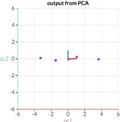
Eigen vectors. This step reduces the dimensionality of our data into a fixed three-dimension space. figure4.1a shows an example data distribution in a 2-D plane andfigure4.1b shows the same data projected into a 2-D Eigen plane. Since Eigen planes are always coplanar, this thus normalizes the data along the same axes.

We can also see from figure 4.1b that maximum variance of data is along thepc1 axis. This makes thepc1 axisthe 1st principal component of the data. Using this property of PCA we can choose the most importantfeaturesonly from a data set while excluding the less importantfeatures. We

see fromfigure4.2a, real data needs both thex and y planeto represent the features (spread) of the data. On the other hand infigure4.2b we can see that most of the variance for the data items has been condensed with negligible variance along thepc2 axis. All features of the data can now be abstracted onto thepc1plane. This method is the method we use for data abstraction while maintaining the features of the data set.

4.2.2 Histogram Generation

Once the dimensionality of the data has been reduced using PCA, we need to reduce the point

(26)

(a)Example: Real Data with 2 Dimensions (b)Example: Data Projected on Eigen Plane

Figure 4.1PCA Projection Example

[Pca]

(a)Example: Variance for Real Data on X and Y axis individually

(b)Example: Variance of Data on PCA axis individu-ally

Figure 4.2Feature Set Abstraction

each dimension having 16 or 32 buckets with ranges computed as follows :

b u c k e t_c o u n t=16o r 32

d i m_b u c k e t_r a n g ed i = m a xd i − m i nd i: ∀d i i n(1 .. 3)

b u c k e t_s i z ed i = d i m_b u c k e t_r a n g ed i /b u c k e t_c o u n t : ∀d i i n(1 .. 3)

b u c k e t_r a n g ej = [(b u c k e t_s i z e∗b u c k e tj+m i nd i),(b u c k e t Si z e∗(b u c k e tj+1) +m i nd i));

∀j i n(1 ..n)

(4.1) This will give us the buckets with their ranges for all dimensions. We then proceed to generate

(27)

E.g.:letthree pointsbe represented in a 3-D Eigen plane by coordinates as follows: p1= (1, 2, 3)p2= (−1, 0, 1)p3= (2, 3, 4)

Now, let there exist 2 buckets per dimension with Ranges as follows:

b11= [−1, 2)b12= [2, 4)b21= [0, 2)b22= [2, 4)b31= [1, 3)b32= [3, 5)

Using the above points and bucket ranges we will now generate3 Histograms(one per dimen-sion) with2 buckets per histogram.The histograms may be represented as follows:

h_p o i n t s1 = b11 : (p1,p2); b12 : (p3); Histogram for first dimension

h_p o i n t s2 = b21 : (p2);b22 : (p1, p3); Histogram for second dimension h_p o i n t s₃ =b₃₁ : (p2); b₃₂ : (p1,p3); Histogram for third dimension

Thus we can see from above example how each item becomes a part of a bucket if its coordinate

for the given dimension lies in the bucket range for that dimension.

4.2.3 Similarity Metric Computation

We now use the Welch’s Test[WEL47][Sie00]to compute the probabilistic metric for similarity and to rank all history data sets wrt to each other and store in decreasing order of similarity. (Note: Will be used in run time historical reuse data set computation.) Welch test is computed for each

dimension of the two sets being matched and the summation of the score for all three dimensions

is as Similarity score for the two data set. Data sets are then ranked with each other based on the similarity score. Higher score means a better and match and vice versa.

4.2.4 Training Algorithm

This part of the algorithm is used to prepare and store data so as to have highest availability of reuse components for all candidates. We try and solve the challenges mentioned in chapter 3

using the methods mentioned in 4.1. Let our history database consist of "n" data sets named:

H D1,H D2, ...H Dn. The following Steps are done for eachH Difor (i in 1 to n) :

• PCA:Compute Eigen vectors forH Di and project data on the Eigen vectors to normalize in

Eigen plane and reduce dimensionality as shown in 4.2.1. We reduce all data into 3-D space for comparison purposes.

• Histogram Generation:Categorize PCA data forH Di buckets for histograms as shown in

4.2.2. One histogram is generated per dimension of data, thus we have a total of 3 histograms

(28)

• Relative Ranking:Use Welch Test to rank all history data sets wrt to each other. Data sets are stored in decreasing order of similarity as shown in Algorithm 1. (Note: Will be used in run

time historical reuse data set computation.)

• Reuse Data for Data Set:Run Algorithm of choice for Data Set and storeComputation Reuse Data. E.g.: In case of the K-means algorithm we choose thefinal centroidscomputed by the K-Means Algorithm for current data set.

Algorithm 1History Data Sets- Relative Ranking

1: procedureRANKHISTORYDATA(H i s t o r y_D a t a b a s e)

2: r e l a t i v e_r a n km a p = O R D E R E D_M AP(Si m i l a r i t y_S c o r e,D a t a_S e t)

3: s c o r e_{F i n a l} =0

4: foreachH Di inH i s t o r y_D a t a b a s e do

5: foreachH Dj inH i s t o r y_D a t a b a s e !=H Dido

6: s c o r e_{F i n a l} =C o m p u t e Si m i l a r i t y(H D_i, H D_j) 7: r e l a t i v e_r a n km a p.i n s e r t(s c o r eF i n a l,H Dj)

8: end for

9: (H D_i).R e l a t i v e_R a n k i n g =r e l a t i v e_r a n k_{m a p} 10: end for

11: end procedure

Algorithm 2Similarity Metric Computation

1: procedureCOMPUTESIMILARITY(D a t a_S e tC u r r e n t,D a t a_S e tH i s t o r i c)

2: s c o r eF i n a l=0

3: D a t aC u r D S=T O P_T H R E E_BU C K E T_D AT A(D a t a_S e tC u r r e n t)

4: D a t aH i s t D S=T O P_T H R E E_BU C K E T_D AT A(D a t a_S e tH i s t o r i c)

5: foreachd i mi inD i m e n s i o n s(D a t a_S e tC u r r e n t)do

6: s c o r eF i n a l+=C a l c W e l c hS c r(D a t aC u r D S.c o l u m n At(d i mi),D a t aH i s t D S.c o l u m n At(d i mi))

7: end for

8: returns c o r eF i n a l

(29)

Algorithm 3Screening Algorithm

1: procedureSCREENING–PRIMARYCANDIDATESELECTION 2: l e a s t_d i s t a n c e_{r a n k}=M AX

3: l e a s t_d i s t a n c er a n g e=M AX

4: d i m_d i s t a n c er a n k=0

5: d i m_d i s t a n c e_{r a n g e} =0 6: H D_R a n ks e l e c t e d

7: H D_R a n g es e l e c t e d

8: foreachH D_xin History Databasedo 9: for eachD i mi w h e r e i i n1 .. 3 do

10: foreachB u c k e tj in Top 3 Buckets(D i mi) in Decreasing Order of Item Count for

current data setdo 11:

12: foreachp tc dandp tH D i in points(B u c k e tj)do

13: d i s t a n c er a n k = d i s t(p tc d, p tH D i);

14: end for

15: B u c k e tk =Bucket inH Di w h e r e r a n g e(b u c k e tk) ∼ r a n g e(b u c k e tj)

16: foreachp tc di n p o i n t s(B u c k e tj)a n d p tH D i i n B u c k e tk do

17: d i s t a n c er a n g e = d i s t(p tc d, p tH D i);

18: end for

19: end for

20: d i m_d i s t a n c er a n k = d i m_d i s t a n c er a n k + d i s t a n c er a n k

21: d i m_d i s t a n c er a n g e = d i m_d i s t a n c er a n g e +d i s t a n c er a n g e

22: end for

23: ifd i m_d i s t a n c e_{r a n k} <l e a s t_d i s t a n c e_{r a n k} then 24: l e a s t_d i s t a n c er a n k =d i m_d i s t a n c er a n k;

25: H D_R a n ks e l e c t e d = H Dx;

26: end if

27: ifd i m_d i s t a n c er a n g e <l e a s t_d i s t a n c er a n g e then

28: l e a s t_d i s t a n c er a n g e =d i m_d i s t a n c er a n g e;

29: H D_R a n g e_{s e l e c t e d} = H D_x;

30: end if

31: end for

(30)

Algorithm 4Best Match Selection Algorithm

1: procedureBESTMATCHSELECTION

2: p r i m a r y_c a n d i d a t e s=S c r e e n i n g–P r i m a r y C a n d i d a t e S e l e c t i o n 3: b e s t_m a t c h_s c o r ef i n a l =I N TMI N

4: b e s t_m a t c h_s c o r ec u r=C o m p u t e Si m i l a r i t y(D a t a_S e tc u r r e n t,p r i m a r y_c a n d i d a t e s[0])

5: b e s t_m a t c hd a t a_s e t =p r i m a r y_c a n d i d a t e s[0]

6: b e s t_m a t c h_s c o r ec u r=C o m p u t e Si m i l a r i t y(D a t a_S e tc u r r e n t,p r i m a r y_c a n d i d a t e s[1])

7: ifb e s t_m a t c h_s c o r ec u r >b e s t_m a t c h_s c o r ef i n a l then

8: b e s t_m a t c h_s c o r ef i n a l =b e s t_m a t c h_s c o r ec u r

9: b e s t_m a t c hd a t a_s e t=p r i m a r y_c a n d i d a t e[1]

10: end if

11: foreachH DxinT O P_T H R E E r e l a t i v era n k(p r i m a r y_c a n d i d a t e s[0])do

12: b e s t_m a t c h_s c o r ec u r=C o m p u t e Si m i l a r i t y(D a t a_S e tc u r r e n t,H Dx)

13: ifb e s t_m a t c h_s c o r ec u r r e n t >b e s t_m a t c h_s c o r ef i n a l then

15: b e s t_m a t c hd a t a_s e t=H Dx

16: end if

17: end for

18: foreachH Dy inT O P_T W Or e l a t i v era n k(p r i m a r y_c a n d i d a t e s[1])do 19: b e s t_m a t c h_s c o r ec u r=C o m p u t e Si m i l a r i t y(D a t a_S e tc u r r e n t,H Dy)

20: ifb e s t_m a t c h_s c o r ec u r >b e s t_m a t c h_s c o r ef i n a l then

22: b e s t_m a t c hd a t a_s e t=H Dy

23: end if

(31)

4.2.5 Computing Best Match for Current Data-set (Run Time)

This is the part of the algorithm that is actually responsible for the selection of the

• PCA:Compute PCA for current Data Set similar to 4.2.4.

• Histogram Generation:We again characterize PCA data into 3 histograms with 32 buckets each as done in 4.2.4.

• Matcher and Selector :The best match data set selection process is divided into 2 parts: screen-ing and final selection. Screenscreen-ing is used to prune our Historical Data Sets to a smaller subset from which we can select our best match Data Set for computation reuse using the final

selection step.

The two parts of the Matcher and Selector part of our algorithm may be defined as follows:

– Screening:This is the process where we select our initial candidates for the next step of our selection algorithm. This part of the algorithm essentially estimates the similarity in distribution for the current and corresponding historical data sets using the Histograms

generated in the previous steps. Variance Similarity is estimated as follows:

1. Take top-k most populated buckets for current data set and select corresponding

top-k bins from all history data sets and top-k buckets with closest min and max to

current data-set top-k bins.

2. Find ED for these data points between current data set and all historical data sets.

3. Choose Historical Data Sets with minimal distance as initial “Best Match” for both

top-k buckets by rank and top-k buckets by range.

Pseudo Code for an understanding of how ourscreening algorithmruns can be seen in

Algorithm 3.

– Find Best Match (Similarity Metric=>Probabilistic Score):One we have found the best match candidates from out screening step, we simple calculate the Welch Test score

for each dimension (d i mi) for each pair of current data set and chosen historic data

sets.

1. Find “Similarity Metric“ as expalined in subsection 4.1.2 and between current data set and above chosen “best match” data sets using Welch’s Test for all dimensions of

all three data sets as shown in Algorithm 2.

(32)

4.3. DISCUSSION CHAPTER 4. HISTORY REUSE ARCHITECTURE

3. Choose Data Set with highest Probability Score.

Pseudo Code for an understanding of how ourfinal selection algorithmruns can be seen

in Algorithm 3.

• Reuse Computations: In this section we use the computational data we had stored for history reuse in the training run for the historical data set selected. For instance, in the case of the K-Means algorithm, we now use the centroids from the chosen historical data set that were

computed during the training run for historical data.

4.3 Discussion

Our final algorithm was reached at after a fair few trials and errors. Some of the major approaches

used apart the latest approach for major challenges may be defined as below:

4.3.1 Computation on Real Data and Incorrect Screening algorithm: 4.3.1.1 Implementation

• In this method I had initially use bin wise reduction on initial (real) data and then used PCA

for dimension reduction of these reduced data points for the calculation of Eigen vectors and

Eigen values only.

• I had then proceeded to run Student’s T-Test for relative ranking in training Run on real data.

• For Run Time computation I had used only the distance between the Eigen vectors for initial screening, choosing the data set with smallest difference in Eigen vectors as initial Best Match

data set.

• I had then proceeded to Use Student T-Test on real data for computation of the probabilistic

metric using all dimensions for the computation of the same.

• Python Numpy Libraries had been used for Student T-Test computation.

• History Reuse component Computations during training run was done on real data of

histori-cal data set instead of PCA data.

4.3.1.2 Reasons for failure

(33)

• Student T-Test worked only with Gaussian Distributions. Garbage value was returned for non Gaussian Data.

• Eigen Vectors of two data set may be orthogonal yet PDF (probability density function) may

be close enough such as to generate similar clusters.

• Use of labels for direct initialization was flawed in the sense that if the data points were jumbled they would produce the wrong order of labels thus still providing a bad match.

• Bin Wise distribution of data points was an expensive operation and computation overhead

increased with increase in dimensionality of data.

• Student T-Test had to compute for multiple dimensions of data and was a time expensive

computation.

4.3.2 Custom CPP Implementation for Welch’s Test

Some of the earlier seen issues were corrected in this section as I noticed that a lot of the run time

improvement was overshadowed by the time taken for choosing the historical data set. I also noticed

that the Student T-Test was not reliable for non-Gaussian data and failed completely in case of different data set sizes. This iteration was also mainly about ensuring quicker run time for the

selection algorithm, so incremental updates were made to optimize the same. Some of the updates

made may be enlisted as follows:

• Implemented Custom Cpp implementation for Welch’s Test to over come overhead created by using python libraries for it and calling python script from Cpp.

• Removed the distribution of data into bins for data point reduction as it had a big overhead in

computation and CPP Welch Test Libraries scaled well for larger data sets.

• Changed to use of Welch’s Test as compared to Student T-Test as Welch’s Test works with non

Gaussian distributed data as well as compared to Student T-Test which makes assumptions of

data distribution being Gaussian in nature.

• For Run Time computation I had used only the distance between the Eigen vectors for initial screening, choosing the data set with smallest difference in Eigen vectors as initial Best Match

data set.

(34)

• Labels for Best Match historic data set were used as-is for current data set.

4.3.3 Random Sampling for Order comparison.

Experimentation on the approach showed non-reliable best match selection. Also I saw that often

the best match might not even yield best results. One of the major reasons for this was the use of

the incorrect use of historical data. For instance, in case of the K-Means algorithm the use of labels instead of the computed centroids lead to dependence on the order of the items in the historic data

set. While the two data set may be similar and produce similar clusters, History Reuse with this method would still fail as initially the data points in current data set may get labeled incorrectly. I

also realized that comparison of non-normalized data was in its very essence. I tried to correct the

above issues with the following methodology:

• Changed implementation to use of PCA data for most computations.

• Projected Historical data set points on Current Data Set Eigen Vectors. Used distance between

data points of Current Data Set and historical data sets by randomly sampling 10% of data sets against each other. Chose Data Set with minimum distance. This was done to try to use

Historical data set with most point order similarity (and thus generated label order similarity)

in conjunction with overall data set similarity.

• Welch’s Test was still used across all dimensions of actual data Similarity Metric Computation.

• Labels were used as-is for real data.

This implementation though corrected some of the above mentioned issues, it in its turn generated

new issues:

• Use of labels for direct initialization was flawed in the sense that if the data points were jumbled they would produce the wrong order of labels thus still providing a bad match.

• Random Sampling was a bad way to judge the order of the labels that would be generated by

K-Means for data set.

• Eigen Vectors of two data set may be orthogonal yet PDF may be close enough such as to

(35)

4.3.4 Use Of PCA Data for Welch’s Test and PCA data for centroid computation in Train-ing Run:

Experimentation still showed both the history reuse to be inconsistent and the overhead of comput-ing historical data set was still quite large. I also realized that while Eigen Vectors of two data set

may be orthogonal yet PDF might be close enough such as to generate similar clusters. To correct

the above issues I used the following methods:

• Used PCA data in training run for Centroid computation of historical data.

• Used PCA data for Welch’s Test based “Similarity Metric” computation.

• Still used labels from best match historical data set as initialization for current data set.

• Stopped projecting historical data sets data on current data set Eigen vectors, instead used

self-projection, which could be done offline.

• Used Random Sampling for initial estimation of best match data set.

The use of Labels was still flawed. Also the use of random sampling was not a very effective

(36)

CHAPTER

5 EVALUATIONS

5.1 Methodology

We have used leave-one cross testing for all experimentations. Most data sets for experimentation are stock databases available on the UCI machine-learning repository while some source data sets

are Microsoft released source data sets for machine learning. These data sources are then divided into data sets. Depending on the size of the data source[Lic13]we may have any where between 10 to 43 data sets, where in all save one are treated as historic data sets. We have also allowed all

algorithms to converge to the same epsilon error rate thus ensuring the run time comparison for similar quality output for algorithms. All experiments have been carried out on Octa core Intel Xeon

CPU E5-2650 Running Ubuntu Linux 14.04 LTS with 16GB of RAM.

5.2 Experiments

To demonstrate the efficacy and efficiency of our program we evaluate our approach by testing it on

various large real world data-sets and compare our algorithm to two most frequently used and vastly

(37)

5.2. EXPERIMENTS CHAPTER 5. EVALUATIONS

based on squared of distance from initial randomly selected center). Both the above algorithms are implemented in the OpenCV library, which has been used as the standard library for Lloyd’s

Algorithm implementation. We run all three algorithms on the same data sets with the same error

rate for convergence. We have also compared the historical data-set selected by our algorithm to all other data-sets available in history to show the accuracy of our algorithm in selecting the best

available data-set.

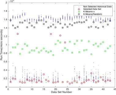
Figure 5.1Hit-Rate (Road Network k=120)

Consistent Selection of Best Match Historical Data-set from History:The experiments run, show that our algorithm is able to consistently able to select one of the top 5 data-sets for history

(38)

Figure 5.2Hit-Rate (Caltec 101 for k=600)

one of the top 5 available data sets with hit rate of above seventy percent across data sets irrespective

of the size and the cluster count. This is expected as we aim to compare data set based on similarity while the cluster count is not taken into consideration in the matching process.Table 5.1shows the

hit rate for our algorithm. We can clearly see from the table that our algorithm is able to select one

of the top 5 best data sets for historical reuse from the available data sets consistently irrespective of the cluster count and the total historically available data sets. This thus validates our theory

for probabilistic selection for matching data sets using theWelch’s Testfor null hypothesis testing for similarity of data sets. We are also able to see clearly that our selection criteria continues to perform well across a wide range of cluster counts and thus validates our hypothesis that data-set

similarity should be used as the primary measure to gauge quality of data-set for history reuse

(39)

Data-set Name History Data-set cnt. Cluster Count Top 5 cnt Hit Rate %

Road Network 43

40 80 120 240 42 41 43 43 97.67% 95.34% 100% 100%

Kegg Network 10

40 80 120 240 8 9 8 8 80% 90% 80% 80%

US Gas Sensor Data 36

40 80 120 240 28 29 29 28 77.7% 80.5% 80.5% 77.7% NotreDame 20 40 80 120 240 17 18 17 17 85% 90% 85% 85% Tiny 20 80 120 240 360 480 600 20 18 16 17 18 18 100% 90% 80% 85% 90% 90%

Uk Bench 20

80 120 240 360 480 600 20 18 16 17 18 18 100% 90% 80% 85% 90% 90%

Caltec 101 20

80 120 240 360 480 600 20 18 16 17 18 18 100% 90% 80% 85% 90% 90%

Table 5.1Selection Hit Rate K-Means History Reuse

(40)

selection algorithm works across various cluster indexes and also how little variation is seen in the performance of the data-sets selected by our algorithm irrespective of the number of clusters(k). We

also show that our hit rate is a minimum of 70 percent (Some error is to be expected as the selection

algorithm works on probabilistic model for making best guess.) Figures 5.1 and 5.2 show how our selected historical data set performs in comparison to all other data sets available for selection in

our history database. We see from them, the accuracy of algorithm in consistently choosing one of the best match data sets from history with high accuracy (> 75%). We see that our algorithm chooses either the best match data set or data set close to best match. This proves the accuracy

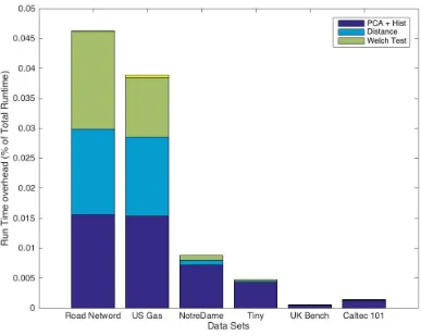
of our algorithm.Consistent Scalable approach to Selection:Our experiments also show that our method scales well with the increase in dimensionality of data(d), the size of the data-set(n)and the cluster count(k).Figures 5.3 and 5.4show our experimental results for various data sets with varying

dimensionality and sizes. These figures clearly show that for any given data set the selection time is

completely independent of the cluster count(k). This is in complete contrast to both therandom K-Means (Lloyd’s Algorithm)and the K-Means++algorithm where the initialization overhead is directly proportional to the cluster count(k)for the data set. Our experimental results also serve the

purpose of showing us that our initialization methodology has an over head very small compared to the total run time of the algorithm even for the smallest of chosen cluster counts. This combined

with the proven choosing of better initialization centroids (as seen in Table 5.2 and Table 5.3 which show an overall improvement in both run time as well as the number of iterations taken for the data

to converge) gives us a win-win situation of a comprehensively better initialization methodology in

comparison to both the previously mentioned methods.

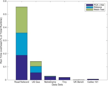
Referencing the above mentioned tables and figures, we can also see that our selection

mecha-nism takes only a very small percentage of the total run time for the algorithm for larger data sets (<0.1%) and while it may be a significant part of the initialization for smaller data sets the quality improvement in the initialization centroids is sufficient to offset the run time for the algorithm to

be a viable initialization methodology for all data sets of varying sizes. Though speed up using our

methodology is seen in all cases, it is best suited for larger data sets, as in that case our overhead for history best match selection almost becomes negligible.

FromFigure 5.5we can also see that even while retaining higher variances for historic data

sets, no further speedup is seen in run time while the introduced overhead becomes a significant percentage for the total run time and may lead to further overheads as data set sizes increase.

Consistent Speed up for K-Means algorithm:The end requirement of any initialization algo-rithm is to ensure that we achieve a consistent speed up over previous approaches. While running our initialization algorithm for K-Means we were able to see consistent speed up in run-time of

(41)

Figure 5.3Best Match Selection Overhead (Maximum for Smallk)

range of cluster counts ranging from 40 to 600. This is though dependent on quality of historical

data sets available. A bad match may lead to relatively bad starting points which in turn leads to an increase in time taken for convergence. Not withstanding the above argument we were able to

see consistently good performance by our algorithm for real data sets. This is largely due to the

normalization of the data sets using the PCA based approach and then using cluster information based on this normalized data rather than the actual data. This also removes the need for the data

to have Gaussian distribution. This gives a higher chance of finding a better historical match, thus

giving consistent speed up over various data sets with different dimensionality(d)and different cardinality(n)for varying cluster countsk.

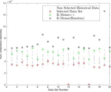
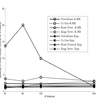
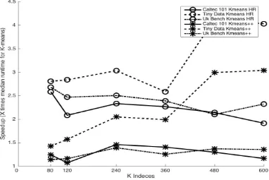
Figures 5.8 and 5.9 shows the range of speed up across various data sets with varying degrees of

(42)

Figure 5.4Best Match Selection Overhead (Minimum for Largek)

graphs that our algorithm consistently outperforms both therandom K-Means(Lloyd’s Algorithm)

and theK-Means++algorithmin run time performance.

Figures 5.6 and 5.7 depict the speed up seen by our algorithm over various cluster sizes for all

data sets. We can see that the general trend is that speed up seen is in general higher for larger

cluster count. This is particularly true because as the cluster count increases we see a speed up in both the initialization method as well as the actual run time because of the improvement seen in

the initialization centroids.

Results seen in Figures 5.3 and 5.4 and Table 5.2 together also show us that the speed ups are consistent irrespective of the cluster counts(k)in terms of both the run time of the algorithms

and the number of iterations taken for the convergence of the algorithm to similar error rate. This

(43)

Figure 5.5Performance for various PCA Dimension Count(Caltec 101; K=600). Default PCA Dims: 3 independent of the cluster index size would lead to sizable improvement in run time. This is so

because run time improvement is seen in both the initialization overhead as well as the actual run time of the algorithm. As the cluster count(k)increases, the amount of initialization overhead for

both the above mentioned initialization methodology becomes a significant part of the total run

time for the algorithm.

Another interesting feature seen in the above box plots is the varying degrees of speed up seen

for the various segments for same data sets. Looking at the speed up thatK-Means with History Reuse

achieves over the originalK-Means (Lloyd’s algorithm)we can see that the speed up is generally spread out over a larger range as compared to the performance of theK-Means++algorithmas

compared toLloyd’s Algorithm. This thus, brings to fore our above made assumption about the

(44)

(45)

Data-set n d k K-Means (TimeµS) K-Means++ K-Means-HRU

Road Net. 1.0E4 3

40 80 120 240 8.5E4 1.6E5 2.01E5 2.4E5 1.7X 2.4X 2.2X 1.8X 6.7X 10.0X 10.0X 1.6X

Kegg Net. 2.0E4 10

40 80 120 240 1.9E5 2.8E6 3.9E5 6.3E5 2.5X 1.9X 1.6X 1.9X 2X 2.2X 2.8X 3.2X

US Gas 1.45E4 13

40 80 120 240 3.2E5 4.7E5 5.2E5 8.9E5 2.4X 1.9X 1.9X 1.7X 5.6X 4.4X 3.9X 4.3X

NotreDame 1.45E4 13

40 80 120 240 2.1E6 3.8E6 5.5E6 1.02E6 1.2X 1.3X 1.3X 1.4X 2.4X 2.3X 2.3X 2.3X

Tiny 1.45E4 13

80 120 240 360 480 600 0.9E8 1.3E8 2.5E8 3.2E8 3.9E8 4.3E8 1.4X 1.6X 2.1X 2.0X 2.9X 2.9X 2.8X 2.9X 3.8X 2.7X 4.1X 4.1X

Uk Bench 1.45E4 13

Caltec 101 1.45E4 13

Table 5.2Runtime comparison: K-Means, K-Means++and K-Means-HRU(*All times inµS)

(46)

Figure 5.7Median Speed up, Large Data (k=600)

box plots above is testament to this. Normalization usingPCAof data sets, tends to mitigate this to a large extent thus providing us the ability to use history data not along same planes as well and thus

providing a consistent speed up, but a better match of normalized data would provide even higher

(47)

Data-set n d k K-Means (Random) K-Means++ K-Means-HRu

Road Net. 1.0E4 3

40 80 120 240 128 119 110 102 69 52 46 79 39 27 30 82

US Gas 1.45E4 13

40 80 120 240 117 111 106 100 58 59 58 55 26 32 33 37

NotreDame 1.45E4 13

40 80 120 240 162 154 132 103 142 114.5 101 74 69.5 65 60 48.5

Tiny 1.45E4 13

80 120 240 360 480 600 195 181.5 168.5 129.5 119.5 111.5 164 154.5 120.5 99.5 87.5 72 108 98 87.5 74 67 58

Uk Bench 1.45E4 13