Initial Results of Using In-Process Testing Metrics to
Estimate Software Reliability
Nachiappan Nagappan
1, Laurie Williams
1,
Mladen Vouk
1, Jason Osborne
21
Department of Computer Science, North Carolina State University, Raleigh, NC 27695
2Department of Statistics, North Carolina State University, Raleigh, NC 27695
{nnagapp, lawilli3, vouk, jaosborn}@ncsu.edu
Abstract
Demand for quality in software applications has grown, and awareness of software testing-related issues plays an important role in that. Unfortunately, in industrial practice, information on field reliability of a product tends to become available too late in the software development process to affordably guide corrective actions. An important step towards remediation of this problem lies in the ability to provide an early estimation of software reliability. This paper presents a suite of in-process metrics that leverages the software testing effort to provide (1) an assessment of potential software field reliability in early software development phases, (2) an intuitive, color-coded, feedback to the developers on the quality of their testing effort, and (3) the identification of software elements that may be fault-prone. A structured experiment conducted at North Carolina State University indicates that our approach is promising. Further studies, predominantly with industrial projects, are being conducted.
Categories and Subject Descriptors
[D.2.8 Metrics]: Reliability metrics, Complexity measures, Performance measures, Process metrics, Product metrics, Software science.
General Terms
Measurement, Performance, Reliability
Keywords
Software Metrics, Software Testing, Software Reliability, Empirical Software Engineering.
1. INTRODUCTION
In industry, estimates of software field reliability are often available too late to affordably guide corrective actions to the quality of the software. True field reliability cannot be measured before a product has been completed and delivered to an internal or external customer. Field reliability is calculated using the number of failures found by these customers. Because this information is available late in the process, corrective actions tend
to be expensive. [6] Software developers can benefit from an early warning regarding the quality of their product.
This early warning can be built from a collection of internal metrics that are correlated with reliability, an external measure. An internal metric, such as the cylomatic complexity [31], is a measure derived from the product itself [25]. An external measure is a measure of a product derived from the external assessment of the behavior of the system [25]. For example, the number of defects found in test is an external measure.
The ISO/IEC standard [25] states that “internal metrics are of little value unless there is evidence that they are related to some externally visible quality.” Internal metrics have been shown to be useful as early indicators of externally-visible product quality [3] because they are related (in a statistically significant and stable way) to the field quality/reliability of the product. The validation of such internal metrics requires a convincing demonstration that (1) the metric measures what it purports to measure and (2) the metric is associated with an important external metric, such as field reliability, maintainability or fault-proneness [16].
Our research objective is to construct and validate a set of easy-to-measure in-process metrics that a) provides meaningful feedback on the thoroughness of a testing effort, and b) can be used as an early indication of an external measure of system reliability. To this end, we have created a metric suite we call the Software Testing and Reliability Early Warning metric suite for Java (STREW-J). The metric suite is applicable for development teams that write extensive automated test cases, such as is done in the Extreme Programming [4] software development methodology. In this paper, we present the results of a study designed to analyze the capabilities of the STREW metrics suite. The study was run with junior- and senior-students in a software engineering class at North Carolina State University (NCSU). The paper is organized as follows. Section 2 discusses the related work. Section 3 outlines the STREW metric suite. Sections 4 and 5 discuss a feasibility study and a formal experiment, in which we studied the STREW metric suite. Section 6 presents the experimental results. Finally, Section 7 and 8 presents the conclusions and future work.
2. BACKGROUND AND RELATED WORK
2.1 Software Reliability
[39] to more sophisticated hyper-geometric coverage-based models [26], to component-based models, and object-oriented models. Several reliability models use Markov Chain techniques [46].
Other models are based on the use of an operational profile, i.e., a set of software operations and their probabilities of occurrence [35]. These operational profiles are used to identify potentially-critical operational areas in the software to signal a need to increase the testing effort in those areas. A large group of software reliability growth models are described by Non-Homogenous Poisson Processes (NHPP) [47]. They include Musa [36] and the Goel-Okumoto [22] models.
In our work, we use the Nelson model where the reliability is given by Equation 1:
Reliability (R) = 1- nf / n, (1) where nf is the number of failures obtained on running a set of test cases, and n is the total number of test cases in this set. In the Nelson model, reliability is viewed as an estimate of the probability the program runs a randomly sampled test case successfully. Standard statistical theory for population proportions then leads to the following 100(1- )% confidence interval for reliability [40], where Z/2 is the upper /2 quantile of the standard normal distribution.
Confidence Interval =
n z
n z n
R R z n z R
2 2 /
2 2
2 / 2
/ 2
2 /
1
4 ) 1 ( 2
α
α α
α
+
+ − ±
+
(2)
2.2 Fault-Proneness and Quality
The higher the failure-proneness1 of the software, the lower the reliability and the quality of the software produced, and vice-versa. Using operational profiling information, it is possible to relate failure-proneness and fault-proneness of a product. Therefore, research on fault-proneness is relevant to our reliability research. Research on fault-proneness has focused on two areas: (1) the definition of metrics to capture software complexity and testing thoroughness and (2) the identification of and experimentation with models that relate software metrics to fault-proneness [13]. While software fault-fault-proneness can be measured before deployment (i.e. the count of faults per structural unit such as faults per line of code), failure-proneness cannot be directly measured on software before deployment [18]. Fault-proneness can be estimated based on directly-measurable software attributes if associations can be established between these attributes and the system fault-proneness.
Structural object-orientation (O-O) measurements, such as those in the CK O-O metric suite [11], have been used to evaluate and predict fault-proneness [3, 7, 8]. These metrics can be a useful early internal indicator of externally-visible product quality [3, 42, 43]. The CK metric suite consist of six metrics: weighted methods per class (WMC), coupling between objects (CBO), depth of inheritance (DIT), number of children (NOC), response for a class (RFC) and lack of cohesion among methods (LCOM).
1 Software fault-proneness is defined as the probability of the presence of faults in the software [13]. Failure-proneness is the probability that a particular software element will fail in operation.
Basili et al. [3] studied the fault-proneness in software programs using eight student projects. They observed that the WMC, CBO, DIT, NOC and RFC were correlated with defects2 while the LCOM was not correlated with defects. Further, Briand et al. [8] performed an industrial case study and observed the CBO, RFC, and LCOM to be associated with the fault-proneness of a class. A similar study done by Briand [7] et al. on eight student projects showed that classes with a higher WMC, CBO, DIT and RFC were more fault-prone while classes with more children (NOC) were less fault-prone. Tang et al. [43] studied three real time systems for testing and maintenance defects. Higher WMC and RFC were found to be associated with fault-proneness. El Emam et al. [17] studied the effect of class size on fault-proneness by using a large telecommunications application. Class size was found to confound the effect of all the metrics on fault-proneness. Finally, Chidamber et al. [10] analyzed project productivity, rework, and design effort of three financial services applications. High CBO and low LCOM were associated with lower productivity, greater rework, and greater design effort. To summarize, there is a growing body of empirical evidence that supports the theoretical validity of the use of these internal metrics [2, 7] as predictors of fault-proneness. The consistency of these findings varies with the programming language [42]. Therefore, the metrics are still open to criticism. [12]
Vouk and Tai [45] showed that in-process metrics have strong correlation with field quality of industrial software products. They demonstrated the use of software metric estimators, such as the number of failures, failure intensity (indicated by failures per test case), and drivers such as change level, component usage, and effort in order to:
(1) quantify component quality in terms of the number of failures expected during initial operational deployment; (2) identify fault-prone and failure-prone components, and (3) guide the software testing process to minimize the number
of failures/faults that can be expected in future phases.
2.3 Analysis Techniques
A number of techniques have been used for the analysis of software quality. For example, multiple linear regression analysis was used to model the dependence of quality on software metrics [28, 34]. The multiple coefficient of determination, R2, provides a quantification of how much variability in the quality can be explained by the regression model. One difficulty associated with multiple linear regression is multicollinearity among the metrics, which can lead to inflated variance in the estimation of reliability. One approach which has been used to overcome this is Principal Component Analysis (PCA). In PCA a smaller number of uncorrelated linear combinations of metrics, which account for as much sample variance as possible, are selected for use in regression (linear or logistic). PCA can be used to select a subset of the metrics (principal components) that maximize variance of the controlling (independent) variable, such as reliability. PCA can be used to remove metrics that are highly correlated with other metrics, thus simplifying data collection with minimal impact on the accuracy of the information provided. A
multivariate logistic regression equation [14] can be built to model the data, using the principal components as the variables. Denaro et al. calculated 38 different software metrics for the open source Apache 1.3 and 2.0 projects. Using PCA, they selected a subset of nine of these metrics which explained 95% of the total data variance.
Discriminant analysis, a statistical technique used to categorize programs into groups based on the metric values, has been used as a tool for the detection of fault-prone programs. Munson et al. [33] used discriminant analysis for classifying programs as fault-prone with a large medical-imaging software system. In their analysis, they also employed the data-splitting technique, where subsets of programs are selected at random and used to train or build a model. The remaining programs are used to quantify the error in estimation of reliability. The data splitting technique is employed to get an independent assessment of how well the reliability can be estimated from a random population sample. Analyses that are based on a single dataset that use the same data to both estimate the model and to assess its performance can lead to unreasonably negative biased estimates of sampling variability. The classification resulting from Munson’s use of discriminant analysis/data splitting was fairly accurate; there were 10% false positives among the high quality programs (incorrectly classified as fault-prone) and 13% false negatives (incorrectly classified as not fault-prone) among the fault-prone programs.
In our work, we utilize discriminant analysis to classify programs based on the STREW metric suite. Additionally, we utilize multiple regression analysis to estimate the reliability of the software programs using the STREW metric elements as the reliability predictors.
3. STREW – JAVA
The STREW is a suite of internal, in-process software metrics that are leveraged to:
• estimate reliability and its confidence interval;
• provide color-coded feedback on the thoroughness of a testing effort; and
• identify fault-prone modules.
The use of the STREW metrics is predicated on the existence of an extensive suite of automated unit test cases being created as development proceeds. Extreme Programmers that practice test-driven development (TDD) [5] write such a test suite. With TDD, software engineers develop production code through rapid iterations of the following steps: (1) writing a small number of automated test cases; (2) running these unit test cases to ensure they fail (since there is no code to run yet); (3) implementing code which should allow the unit test cases to pass; (4) re-running the unit test cases to ensure they now pass with the new code; (5) refactoring [20] implementation and test code, as necessary; and (6) periodically re-running all the test cases in the code base to ensure the new code does not break any previously-running test cases. In these iterations, test cases will almost always fail initially (because test code is written prior to implementation code) but all test cases will ultimately pass. These automated test cases serve as regression tests [24].
Currently, the STREW Version 1.3 consists of the seven candidate metrics. The metrics are intended to cross-check each other and to triangulate upon a reliability estimate. For example, one developer might write fewer test cases, each with multiple asserts checking various conditions. Another developer might test
the same conditions by writing many more test cases, each with only one assert. We intend for our metric suite to provide useful guidance to each of these developers without prescribing the style of writing the test cases. The seven metrics are now described:
•number of test cases/source lines of code (R1) is an indication of whether there are too few test cases written to test the body of source code;
•number of test cases/number of requirements (R2) is an indication of the thoroughness of testing relative to the requirements;
•test lines of code/source lines of code (R3) is an indication of whether the ratio R1 was misleading as there might have been fewer, but comprehensive, test cases;
•number of assertions/source lines of code (R4) serves as a crosscheck for both R1 and R2 because there are few test cases but each have a large number of assertions [41]; •number of test classes/number of source classes (R5) is an
indication of how thoroughly the source classes have been tested;
•number of conditionals (for, while, if, do-while, switch )/ number of source lines of code (R6) is an indication of the extent to which conditionals (measured by cyclomatic complexity [31]) are used. The use of conditional statements increases the amount of testing required because there are more logic and data flow paths to be verified [27];
•number of lines of code/number of classes (R7) is used as an indicator for estimating reliability when prior releases of the software are available so that any change in the relative class size can be analyzed to determine if the increase in the size of the class has be accompanied by a corresponding increase in the testing effort [17].
We have automated the collection and analysis of the STREW metrics via an open source Eclipse3 plug-in [37]. In addition to providing a reliability estimate, the tool provides color-coded feedback on the quality of the testing effort relative to historical data from comparable projects. Color coding aids developers in quickly understanding if a metric is within acceptable limits. The color choice is determined by the results of Equation 3 for each metric. The use of this equation is predicated on a normal distribution of defects. If the defects are not normally distributed, the Box-Cox normal transformation can be used to transform the non-normal data into normal form. [40] Using historical data from comparable projects that were successful, the lower limit (LL) of each metric ratio is calculated using Equation 3. The mean of the historical values for each metric serves as the upper limit. The color-coded feedback works in reverse for ratio R7 because the larger the size of a class the higher the possibility of errors [17]. The historical data is computed from previously-successful projects with acceptable levels of reliability. Preferably, historical values are calculated per person, since the values depend upon personal coding styles. In the absence of historical data, standard values can be used; we will develop these standards via future program analyses of academic and industrial systems.
LL(Rx) = x-z /2*Standard deviation of metric Rx (3)
n
RED: Rx < LL (Metric) ORANGE: LL (Metric) Rx x GREEN: Rx > x
whereLL = Lower Limit; x = Mean of metric x; Rx is metric id.
4. FEASIBILITY STUDY AND RESULTS
We ran a feasibility study on 13 vending machine programs written in Java by junior/senior-level undergraduates in a software engineering course at NCSU in Fall 2002. The programs were, on average, 789 lines of code (LOC). With these programs, we analyzed an initial set of metrics defined in the STREW-J Version 1.1 [38] based on a subset of the Version 1.3 metrics:•number of test cases/source lines of code (R1);
•number of test cases/number of requirements (R2);
•test lines of code/source lines of code (R3); •number of asserts/source lines of code (R4); and on •statement coverage (C).
There are several overlapping metrics intended to crosscheck each other and to triangulate upon the quality of the testing effort. We estimated reliability via the no failure model described by Hamlet et al. [23] and others [15, 32]. This model was chosen because the programmers worked until all the automated test cases passed (e.g. no failures are demonstrated by the test suite). However, it is possible and even likely that the test suite does not constitute a thorough test effort. To use the no failure model, we must identify a meaningful long term failure rate denoted by and that N random tests have established an upper confidence bound (1- ) that is below some level [23]. The relationship between these factors is given by 1- (1- )N <= [44]. This model is similar to the analysis performed by Frankl et al. [21] on operational testing given by 1-(1-q)T, where q is the failure rate for operational testing and T is the number of tests.
We ran a multiple regression analysis with the metrics collected from the program and the reliability estimate. The result of applying an ordinary least squares regression provided evidence (F=4.325, p=0.041) of a linear association between the reliability estimate and the metrics. The regression equation to predict the reliability was found to be:
Reliability = 0.669 + 1.586*R1 + 0.0513*R2 – 0.0290*R3 +
0.192*R4 – 0.0774*C (4)
Correlations between the metrics and the reliability estimate for various values of are given in Table 1. The given p-values for tests of zero correlation provide evidence of positive linear dependence of reliability on the metrics R1 and R2. Ratios R3 and R4 are not statistically significant4. This may be because the coefficients were based upon programs from a small number (N=13) of different programmers and the value of R3 and R4 relies on personal programming style. The relationship between the code coverage and the estimated reliability was also not statistically significant. This might be because the students were specifically assigned to create test suites with 100% statement coverage which may have artificially altered the results. While only R1 and R2 demonstrated a statistically significant relationship, we will continue to analyze the potential of the other metrics in our on-going analysis.
4 Throughout the paper, we use a 95% confidence level for statistical
significance.
Table 1: Pearson correlation and statistical significance results between the ratios and the reliability estimate
R1 R2 R3 R4 Coverage
0.01 0.629,
p=.021 p=.000 0.992, p=.316 0.302, p=.106 0.469, p=.702 0.118, 0.05 0.703,
p=.007 p=.001 0.814, p=.184 0.393, p=.056 0.541, p=.900 0.039, 0.10 0.616,
p=.025 p=.036 0.584, p=.159 0.414, p=.081 0.502, -0.071, p=.817
5. STRUCTURED EXPERIMENT
A two-phased experiment was carried out in a junior/senior-level software engineering course at NCSU in the fall 2003 semester. The first phase provided the historical data for the second phase.
5.1 Research Design
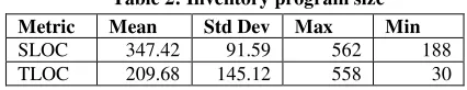
In the first phase, an initial multiple linear regression model was built and test quality feedback standards were calculated based on a set of Java programs written by students working individually over a three-week period. The programs implemented a simplistic inventory system. The students wrote unit test cases using the JUnit5 testing framework. The assignment stated that 100% statement coverage was required. Thirty one working programs with test cases were used for the analysis. The size of the inventory program in terms of the source lines of code (SLOC) and test lines of code (TLOC) is shown in Table 2.
Table 2: Inventory program size Metric Mean Std Dev Max Min
SLOC 347.42 91.59 562 188
TLOC 209.68 145.12 558 30
The multiple regression model and test quality feedback standards were constructed using these programs. The programs were tested against a fixed set of six black-box test cases and the reliability of the system was calculated via the Nelson model.
In the second phase, the students developed an open source Eclipse plug-in in Java that automated the collection of project metrics. Each project was developed by a group of four or five junior or senior undergraduates during a six-week final class project. The plug-in was required to have 80% statement coverage in their JUnit unit test suite. A total of 22 projects were submitted; all were used in the analysis. Table 3 below shows the size of the projects developed in terms of the SLOC and the TLOC.
Table 3: Eclipse project size
Metric Mean Std Dev Max Min
SLOC 1996.9 835.9 3631 617
TLOC 688.7 464.4 2115 156
The plug-ins were evaluated using a comprehensive set of 31 black-box test cases. Twenty six of these were acceptance tests and were given to the students during development. The 31 test cases included exception checking, error handling, and five boundary test cases that checked the operational correctness of the plug-in. The Nelson model was used for reliability estimation.
5.2 Experimental Limitations
An external validity issue arises because the programs were written by students. This concern is mitigated to some degree
because the students were advanced undergraduates (junior/senior). Some of the students have had industry experience. Additionally, both the inventory program and the Eclipse plug-in are small relative to industry applications. Internal validity issue arises because the students worked alone and were learning to use JUnit in the inventory program. The Eclipse plug-in and its associated testing were more complex than the inventory program. For one of our analysis schemes, the metrics collected during this learning phase were used as the historical data for the second phase. Finally, there is a potential construct validity concern with the R2 metric that uses the number of requirements. We have found that this metric can be subjective for some industrial teams because requirements are sometimes evolved, added, and/or deleted without formal documentation being changed. Additionally, we calculated actual reliability by running black box test cases as an approximation of field reliability.
We provide initial results of using in-process metrics for the three purposes outlined in Section 3. Our current findings are not conclusive but indicate that our approach is promising. Further studies, predominantly with industrial projects, are being conducted.
6. EXPERIMENTAL RESULTS
In this section, we discuss the results of utilizing the experimental data to estimate reliability, to provide test quality feedback, and to identify fault-prone programs. We perform this analysis6 in two ways. First, we use the results of the inventory programs to develop historical values for use with the Eclipse projects. Secondly, we use data splitting to analyze the Eclipse projects. We also identify fault-prone among the inventory programs and the Eclipse projects. Equation 3 was applied to the number of failures detected by the test cases to calculate the lower limit on the number of failures. Those programs and projects that had fewer failures than the calculated lower limit were classified as not fault-prone (N-FP), and the remaining programs were classified as fault-prone (FP).
6.1 Model Building and Test Quality Feedback
The following sections illustrate the use of multiple regression analysis of the 31 inventory programs to develop a regression equation for reliability estimation and to calculate standards for the STREW metrics.6.1.1 Multiple Regression Analysis
Using the system reliability obtained by the Nelson model as the dependant variable and the remaining seven metrics as predictors, a multiple regression analysis was performed. Multiple regression Equation 5 was developed.
Reliability Estimate = 0.859 + 0.09459*R1 + 0.01333*R2 - 0.0404*R3 + 1.674*R4 + 0.01242*R5 - 1.222*R6 +
0.000867*R7 (5)
The F-ratio to test the hypothesis that all regression coefficients are zero was not statistically significant (F = 1.653; p = 0.171). The non-significance of this F-ratio is due to over fitting and
6NOTE: SPSS was used for the purpose of statistical analysis. SPSS does not provide statistical significance beyond 3 places of decimal. p=0.000 is interpreted as p<0.0005.
multicollinearity among the metrics. Investigation of marginal correlations reveal significant positive associations between estimated reliability and the metrics R1 (p =0.0424); R3 (p = 0.0293) and R4 (p = 0.0018). To account for our use of every single metric in the regression equation, we calculate the Mallow’s Cp statistic [30] to choose a subset of the metrics. The Mallow's Cp statistic can be used to search for more parsimonious models until more data is available to overcome the inflated variance caused by multicollinearity. Table 4 shows the computed Mallows Cp statistic, the dfMLR (Model degrees of freedom which is equal to the number of variables in the equation) and dfE (Error degrees of freedom that is equal to N-1- dfMLR). Further, as shown below in table 4, the computed Mallow's statistic for all the subsets (N=127 models) led us to the model that included the three metrics (R4, R6, R7) that had practically the same R2 (as the model with all the 7 metric ratios) but had a statistically significant F ratio of F = 4.48; p = 0.011. The next model comprising of metrics R3, R4, R6, and R7 is included for completeness to indicate the comparable values of the F-ratio and the R2. Thus we continue with the initial regression model defined in equation 5 but we plan to collect more data needed to accurately calibrate the model and account for multicollinearity and over fitting.
Table 4: Mallow Cp statistics
Metrics in
the Model ratio F- value p- dfE dfMLR Cp R
2
R1,R2,R3,R
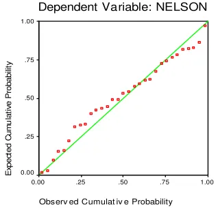
4,R5,R6,R7 1.653 0.171 23 7 8 0.335 R4,R6,R7 4.48 0.011 27 3 0.08 0.3325 R3,R4,R6,R7 3.25 0.028 26 4 2.06 0.3327 Figure 1 below shows the normal probability plot of the regression standardized residual using the reliability as the dependent variable.
Dependent Variable: NELSON
Observ ed Cumulat iv e Probability 1.00 .75 .50 .25 0.00
E
xp
ec
te
d
C
um
u
la
tiv
e
P
ro
ba
bi
lit
y
1.00
.75
.50
.25
0.00
Figure 1: Normal probability plot of the regression standardized residual
6.1.2 Test Quality Feedback Standards
indicate that we can accept the null hypothesis. We applied Equation 3 to the 31 inventory programs and developed standards for the seven metric values, as shown in Table 5. These standards were used to provide color-coded feedback on the quality of the testing effort for the Eclipse plug-in projects.
Table 5: Test quality feedback standards Metric Lower Limit Mean
R1 0.0319 0.0518
R2 0.5192 0.8698
R3 0.5128 0.7674
R4 0.0558 0.0982
R5 0.7478 0.8897
R6 0.1325 0.1509
R7 57.2176 65.6158
6.2 Analysis Using Historical Values
We analyzed the 22 Eclipse projects using multiple regression Equation 5 developed in section 6.1.1 and the test quality feedback standards developed in section 6.1.2.
6.2.1 Multiple Regression
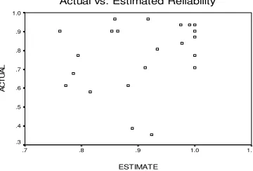
Using Equation 5 and the metrics values calculated for the project, we estimated the empirical reliability of the projects. First, a one sample Kolmogorov-Smirnov test on the defect results (Z=0.807, p=0.533) indicated that we can accept the null hypothesis that the defect population distribution is normal. We approximated the actual reliability using the Nelson model. The reliability estimate was computed using regression Equation 5. As shown in the Figure 2 scattergram, the reliability estimate and the actual values are comparable except in five cases wherein the actual reliability is lower than the predicted reliability. In four of these five cases (projects 8, 11, 12, 20), the ratio of test code to source code was .2 or less. The other 17 programs had a mean ratio of 0.4. Our findings suggest that a minimum ratio of 0.4 is advisable for our metric suite to provide a useful reliability estimate. In the fifth case (project 6), the students misinterpreted the requirements and produced a product that failed several test cases. This singular observation may suggest the method may not be accurate when used with very fault-prone programs. To analyze the relationship between the estimated and actual reliability, we ran a Spearman correlation analysis. The results (correlation coefficient =0.241, p=0.279) indicated that, though not statistically significant, the estimated and actual reliability have a positive relationship wherein an increase in estimated reliability is accompanied by an increase in actual reliability.
Actual vs. Estimated Reliability
ESTIMATE
1.1 1.0
.9 .8
.7
A
C
T
U
A
L
1.0
.9
.8
.7
.6
.5
.4
.3
Figure 2: Actual reliability vs. regression estimated reliability
Using the Equation 3 for the confidence interval, the actual reliability is comparable to the estimated confidence intervals as shown by the lower limit (LL) and the upper limit (UL) in Figure 3. This suggests the estimated reliability is an efficient indicator of the actual reliability.
Actual Reliability vs. Estimated
Reliability Confidence Intervals
Projects
21 19 17 15 13 11 9 7 5 3 1
R
el
ia
bi
lit
y
1.2
1.0
.8
.6
.4
.2
ACTUAL EUL ELL
Figure 3: Actual reliability vs. reliability confidence intervals
6.2.2 Test Quality Feedback
The test quality standards, shown in Table 4 and the inventory programs, were used to provide color-coded feedback on the thoroughness of the test effort of the Eclipse projects. Table 6 shows the results of this color-coded feedback for the 22 projects.
Table 6: Color-coded test quality feedback per program
Quantity of Feedbacks per Color
Project Num.
Red Orange Green
Classified Fault-prone
1 0 1 6 Yes
2 4 1 2 No
3 5 0 2 Yes
4 4 2 1 No
5 3 1 3 No
6 5 0 2 Yes
7 2 4 1 No
8 6 0 1 Yes
9 2 2 3 No
10 5 0 2 No
11 4 2 1 Yes
12 3 1 3 Yes
13 3 2 2 Yes
14 5 2 0 No
15 5 1 1 Yes
16 1 3 3 Yes
17 4 0 3 No
18 4 1 2 No
19 5 0 2 No
20 5 0 2 Yes
21 3 2 2 No
Fault-prone programs were identified by using the number of failures obtained from running the fixed set of test cases and applying Equation 3 to calculate lower bounds for the failures. The plug-in projects that have fewer failures than the lower bound are classified as not fault-prone and vice versa.
To assess the association between the color-coded feedback and the actual reliability of the system, we ran a Spearman rank correlation. The Spearman rank correlation is a commonly-used robust correlation technique [19] because it can be applied even when the association between elements is non-linear; the Pearson bivariate correlation requires the data to be distributed normally and the association to between elements to be linear. The correlation results indicate that the Spearman rank correlation coefficient ( ) between the reliability and the number of red and orange color feedback is negative ( = -0.145, p = 0.516) though not statistically significant. The negative correlation indicates the desired relationship: the more red and orange feedbacks, the lower the system reliability. Correspondingly the correlation coefficient between the number of green feedbacks and the actual reliability is positive ( =0.145, p=0.519), implying the more green feedback, the higher the reliability.
Thus, from these results we can conclude that there exists an indicative relationship between the color-coded feedback and the actual reliability of the software. Hence, the color-coded feedback can provide developers a visual indication of the components and/or programs that might require additional testing. The upper and lower limit values will be further investigated and calibrated with future projects.
6.3 Data Splitting
For comparison, we re-perform the analysis using the data splitting approach. This analysis may be preferred over using the historical values since there are learning issues as discussed in Section 5.2.
6.3.1 Multiple regression approach
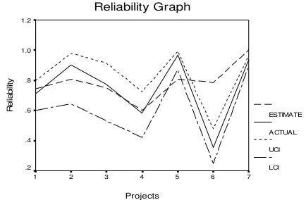
From the available 22 programs, 15 projects were randomly selected7 to build the multiple regression model. The model had a high R2 value of 0.612 that indicated the model was a good fit for the available data. Figure 4 below shows the fit of the reliability estimate according to the regression equation and the actual reliability calculated using the Nelson model. The upper and lower confidence intervals for the actual reliability are also shown. The reliability estimated by our regression equation is comparable with the actual reliability of the system demonstrated by a Spearman correlation analysis between the actual and estimated reliability ( = 0.750, p = 0.052).
7 using a pseudo random generator http://www.randomizer.org/index.htm
Reliability Graph
Projects
7 6 5 4 3 2 1
R
el
ia
bi
lit
y
1.2
1.0
.8
.6
.4
.2
ESTIMATE ACTUAL UCI LCI
Figure 4: Actual vs. regression estimate of reliability
6.3.2 Test Quality feedback
Using another set of pseudo random numbers, 15 projects were selected to form the standards for the test quality feedback. These standards are shown in Table 7. Using these standards, the remaining seven projects were evaluated. The color-coded feedback results are shown below in Table 8.
Table 7: Test quality feedback standards Metric Lower Limit Mean
R1 0.0179 0.0285
R2 2.0472 4.1897
R3 0.2309 0.3850
R4 0.0295 0.0608
R5 0.4465 0.6020
R6 0.1281 0.1530
R7 91.8568 114.2658
Table 8 indicates that the fault-prone projects have a higher amount of red and orange feedbacks (except for project 3 that has a test code to source code ratio of 0.09) compared to the non-fault-prone programs. Excluding project 3 from the analysis we see that a Spearman correlation analysis yields = -0.559, (p = 0.249) between the number of red/orange feedbacks and actual reliability that indicates that with the increase in the number of red/orange feedbacks there is a decrease in system reliability. Similarly the correlation results ( = 0.559, (p = 0.249)) between the number of green feedbacks and the actual reliability indicates that the system reliability increases with the increase in the number of green feedbacks. The sample size of seven projects is too small to run a correlation analysis to draw any meaningful statistically significant results but these results confirm the observations in section 6.2.2.
Table 8: Color coded feedback for projects
Quantity of Feedbacks per Color
Project
Number Red Orange Green Classified Fault-prone
3 2 0 5 Yes
4 2 1 4 Yes
7 1 5 1 Yes
13 0 4 3 Yes
15 1 3 3 No
16 0 2 5 No
6.4 Discriminant Analysis
We used discriminant analysis to identify fault-prone programs based on the metric suite elements.
6.4.1 Analysis I – Inventory programs
Applying Equation 3 to the inventory programs, we classified the programs with more than one failure as fault-prone and the others were classified as not fault-prone. As shown in Table 9, analysis of variance revealed that the metrics R1, R2, R3, and R4 have a significant effect on the characterization of a program as fault-prone or not. But, the metrics R5, R6, and R7 did not produce statistically significant results. This result is as expected because the effectiveness of these metrics increases when testing different releases of the same product.
Table 9: Univariate ANOVA between the fault-proneness and the metric suite elements
Metric F-statistic Significance
R1 8.00 p=0.008
R2 6.038 p=0.020
R3 7.732 p=0.009
R4 8.830 p=0.006
R5 1.930 p=0.175
R6 0.068 p=0.796
R7 1.179 p=0.287
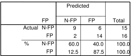
Further, the discriminant analysis produces an acceptable eigen value (0.481) for the given data; the eigen value measures how well the discriminant function discriminates between the categories. The effectiveness of the discriminant analysis is demonstrated in Table 10. The discriminant analysis was successful in correctly classifying 74.2% ((9+14)/31) of the programs. Fourteen of the 16 fault-prone programs were correctly classified, i.e. 87.5% (14/16).
Table 10: Inventory classification Results
6.4.2 Analysis II – Eclipse plug-in projects
Discriminant analysis of the 22 Eclipse projects also yielded a high eigen value (1.839) for the discriminant function. This indicates that the function was effective in classifying the fault-prone components. The classification results, as shown in Table 11, indicating that overall 90.9% of the projects were properly classified.
These results illustrate the efficacy of the discriminant analysis technique for the identification of fault-prone programs based on their internal metric values. Regular use of such information can help organizations indentify fault-prone programs/modules, and improve their testing process.
Table 11: Eclipse project classification results
6.5 Cross Correlation
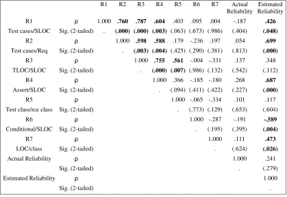
The STREW metrics are intended to provide a cross-check on each other to triangulate upon a reliability estimate. Additionally, the metrics should provide a consistent direction and should not contradict each other (whereby improving one is to the detriment of another). To analyze the relationship among the metrics, we ran a Spearman rank correlation among the metrics using the 31 inventory programs, the results of which are shown in table 12. We identify the presence of a relationship between the metric suite elements if the Spearman correlation coefficient is statistically significant at 95% confidence (p<0.05).
From Table 12 we can observe the following relationships between the metric suite elements.
Relation 1: R1 R2, R3, R4, R5. Relation 2: R2 R3, R4, R5. Relation 3: R3 R4, R5. Relation 4: R4 R5, R6 Relation 5: R6 R7
For example, Relation 1 indicates that there exists a statistically significant relationship between R1 and R2, R3, R4 and R5 and vice-versa, i.e. between R5, R4, R3, R2 and ratio R1. Using a similar selection criterion, Table 13 displays the following relationships between the metric suite elements.
Relation 1: R1 R2, R3, R4, R5. Relation 2: R2 R3, R4. Relation 3: R3 R4, R5.
The comparison of the three relations obtained from the 22 Eclipse projects and the five relations obtained from the 32 inventory programs indicates that there exists a correspondingly similar set of relations, though not the same relations, between the two sets of data. Thus, this analysis serves to demonstrate a more general cross-correlation among the ratios, indicating they are not giving conflicting information.
7. CONCLUSIONS
Feedback on potential field reliability information of software is very useful to developers because it helps identify weaknesses and faults in the software that require fixing. However, in most production environments, field reliability is measured too late to affordably guide significant corrective actions In this paper we have reported on an initial metric suite for providing an early warning regarding system reliability, as well as providing the developers with some feedback on the thoroughness of their testing effort, and for identifying fault-prone programs.
9 6 15
2 14 16
60.0 40.0 100.0
12.5 87.5 100.0
FP N-FP FP N-FP FP Ac Actual
%
N-FP FP
Predicted
Total
10 1 11
1 10 11
90.9 9.1 100.0
9.1 90.9 100.0
FP N-FP FP N-FP FP Ac Actual
%
N-FP FP
Predicted
Table 12: Cross correlation among the STREW metric elements (inventory programs)
R1 R2 R3 R4 R5 R6 R7 Actual
Reliability
R1 1.000 .953 .763 .813 .455 .160 .141 .953
Test cases/SLOC Sig. (2-tailed) . (.000) (.000) (.000) (.010) (.388) (.449) (.000)
R2 1.000 .758 .757 .402 .121 .160 1.000
Test cases/Req Sig. (2-tailed) . (.000) (.000) (.025) (.518) (.391) .
R3 1.000 .796 .523 .298 .029 .758
TLOC/SLOC Sig. (2-tailed) . (.000) (.003) (.104) (.878) (.000)
R4 1.000 .433 .415 -.025 .757
Assert/SLOC Sig. (2-tailed) . (.015) (.020) (.895) (.000)
R5 1.000 -.162 .350 .402
Test class/rce class Sig. (2-tailed) . (.384) (.054) (.025)
R6 1.000 -.403 .121
Conditional/SLOC Sig. (2-tailed) . (.025) (.518)
R7 1.000 .160
LOC/class Sig. (2-tailed) . (.391)
Actual Reliability 1.000
Sig. (2-tailed) .
Table 13: Cross correlation among the STREW metric elements (Eclipse projects)
R1 R2 R3 R4 R5 R6 R7 Actual
Reliability Reliability Estimated R1 1.000 .760 .787 .604 .403 .095 .004 -.187 .426
Test cases/SLOC Sig. (2-tailed) . (.000) (.000) (.003) (.063) (.673) (.986) (.404) (.048)
R2 1.000 .598 .588 .179 -.236 .197 .054 .699
Test cases/Req Sig. (2-tailed) . (.003) (.004) (.425) (.290) (.381) (.813) (.000)
R3 1.000 .755 .561 -.004 -.331 .137 .348
TLOC/SLOC Sig. (2-tailed) . (.000) (.007) (.986) (.132) (.542) (.112)
R4 1.000 .366 -.185 -.180 .268 .687
Assert/SLOC Sig. (2-tailed) . (.094) (.411) (.422) (.227) (.000)
R5 1.000 -.065 -.334 .101 .117
Test class/rce class Sig. (2-tailed) . (.773) (.129) (.653) (.604)
R6 1.000 -.287 -.191 -.589
Conditional/SLOC Sig. (2-tailed) . (.195) (.395) (.004)
R7 1.000 .111 .473
LOC/class Sig. (2-tailed) . (.624) (.026)
Actual Reliability 1.000 .241
Sig. (2-tailed) . (.279)
Estimated Reliability 1.000
We ran a feasibility study and a two staged experiment to examine the ability of the STREW metric suite to fulfill these three goals. Our results are summarized in Table 14.
Table 14: Results summary Feas.
Study Inventory Historical Eclipse Eclipse Data Split
Reliability
Estimate F=4.325, p=0.041 (p=0.171) F=1.653, N/A F=1.578, p=0.281 Test
Feedback N/A N/A Or/Red: = -.145, (p=0.516) Green: =0.145, (p=0.519)
Or/Red: = -.559, (p=0.249) Green: =0.559, (p=0.249) Identify
FP N/A All: 74% FP: 87%
All: 90.9% FP: 90.9% The main observations are:
• A multiple regression approach for empirical reliability estimation using the STREW metric suite is a practical approach to measuring software reliability;
• Feedback provided to developers on the quality of their testing effort, based on the STREW metric elements, is a reflection of the reliability (and by implication fault-proneness) of the program;
• STREW-based discriminant analysis is a feasible technique for detecting fault-prone programs; and • The metric suite elements demonstrate a statistically
significant degree of cross correlation, confirming that the metrics are not giving conflicting information.
In determining the composition of our metric suite, we examined the correlation between each of the metrics and reliability. These results are summarized in Table 15.
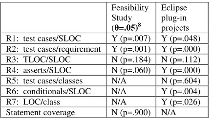
Table 15: correlation of metrics with reliability estimate
Feasibility Study ( =.05)8
Eclipse plug-in projects R1: test cases/SLOC Y (p=.007) Y (p=.048) R2: test cases/requirement Y (p=.001) Y (p=.000) R3: TLOC/SLOC N (p=.184) N (p=.112) R4: asserts/SLOC N (p=.060) Y (p=.000) R5: test cases/classes N/A N (p=.604) R6: conditionals/SLOC N/A Y (p=.004) R7: LOC/class N/A Y (p=.026) Statement coverage N (p=.900) N/A
Based on the results of our analysis we can say that the metric ratios R1 to R5 look promising. We will examine the efficacy of the metric suite elements R6 and R7 based on further case studies.
8. FUTURE WORK
We will continue to refine the metric suite by add/deleting new metrics based on the results of further studies. One metric that will be investigated is code coverage. Code coverageindicates the extent to which a source program has been exercised and
8 The reliability estimate according to the zero failure model was used.
performs a cross check on the value of R3. Popular coverage measures include statement, branch, and conditional coverage. Coverage, in combination with appropriate exposure, has been found to be an effective estimator of software reliability [9]. Additionally, studies have shown an increase in system reliability with an increase in test coverage [29]. We also plan to examine all programs using the metrics that comprise of the CK metric suite. Of interest is, for example, which subset of the CK and STREW metric suites will be an effective indicator of reliability and fault-proneness. Furthermore, we also plan to assess, in the context of our suite, the relationship between traditional software metrics, such as LOC and cyclomatic complexity and system reliability. The metric suite STREW Version 1.4 already is augmented with these metrics. Future analyses will include these metrics.
We will continue to validate the metric suite under different industrial and academic environments. There also arises the need to generalize the STREW-J for other object oriented languages with more case studies. We also propose to evaluate the suite of metrics using different analysis techniques, like logistic regression and PCA, to determine the most appropriate and minimal set of metrics for the STREW metric suite. Finally, we will develop standards for these metrics, so that developers can compare their program reliabilities in a meaningful was, and get feedback on the quality of their testing effort relative to industry developed standards.
Acknowledgements
This work was funded by an IBM Eclipse Innovation Award. We would like to thank the members of the North Carolina State University Software Engineering Reading Group and Amit Paradkar of IBM T.J.Watson Research Center for reviewing initial drafts of this paper.
References
[1] "IEEE Std 982.2-1988 IEEE guide for the use of IEEE standard dictionary of measures to produce reliable software," 1988.
[2] Basili, V., L. Briand, and W. Melo, "A Validation of Object Oriented Design Metrics as Quality Indicators," IEEE Transactions on Software Engineering, vol. 22, pp. 751-761, 1996.
[3] Basili, V., Briand, L., Melo, W., "A Validation of Object Oriented Design Metrics as Quality Indicators," IEEE Transactions on Software Engineering, vol. Vol. 22, pp. 751 - 761, 1996.
[4] Beck, K., "Extreme Programming Explained: Embrace Change." Reading, Massachusetts: Addison-Wesley, 2000. [5] Beck, K., Test Driven Development- by Example. Boston:
Addison-Wesley, 2003.
[6] Boehm, B. W., Software Engineering Economics. Englewood Cliffs, NJ: Prentice-Hall, Inc., 1981.
[7] Briand, L. C., Wuest, J., Daly, J.W., Porter, D.V., "Exploring the Relationship between Design Measures and Software Quality in Object Oriented Systems," Journal of Systems and Software, vol. Vol. 51, pp. 245-273, 2000.
[8] Briand, L. C., Wuest, J., Ikonomovski, S., Lounis, H.,, "Investigating quality factors in object-oriented designs: an industrial case study," presented at ICSE, 1999.pp. 345-354 [9] Chen, M.-H., Lyu, M.R., Wong, "An empirical study of the
estimation," presented at Third International Software Metrics Symposium, 1996.pp. 133 - 141
[10] Chidamber, S. R., Darcy, D.P., Kemerer, C.F.,, "Managerial Use of Metrics for Object Oriented Software: An Exploratory Analysis," IEEE Transactions on Software Engineering, pp. 629-639, 1998.
[11] Chidamber, S. R. and C. F. Kemerer, "A Metrics Suite for Object Oriented Design," in IEEE Transactions on Software Engineering, vol. 20, 1994.
[12] Churcher, N. I. and M. J. Shepperd, "Comments on 'A Metrics Suite for Object-Oriented Design'," in IEEE Transactions on Software Engineering, vol. 21, 1995, pp. 263-5.
[13] Denaro, G., Morasca, S., Pezze, M., "Deriving Models of Software Fault-Proneness," presented at SEKE 2002, 2002.pp. 361-368
[14] Denaro, G., Pezze, M., "An empirical evaluation of fault-proneness models," presented at International Conference on Software Engineering, 2002.pp. 241 - 251
[15] Ehrenberger, W., "Statistical Testing of Real-Time Software," in Verification and Validation of Real-Time Software, W. Quirk, J., Ed. New York: Springer-Verlag, 1985.
[16] El Emam, K., "A Methodology for Validating Software Product Metrics." Ottawa, Ontario, Canada: National Research Council of Canada, June 2000.
[17] El Emam, K., Benlarbi, S., Goel, N., Rai, S.N., "The Confounding Effect of Class Size on the Validity of Object-Oriented Metrics," IEEE Transactions on Software Engineering, vol. Vol. 27, pp. 630 - 650, 2001.
[18] Fenton, N., Neil, M., "A critique of software defect prediction models," IEEE Transactions on Software Engineering, pp. 675-689, 1999.
[19] Fenton, N. E., Pfleeger, S.L., Software Metrics. Boston, MA: International Thompson Publishing, 1997.
[20] Fowler, M., K. Beck, J. Brant, W. Opdyke, and D. Roberts, "Refactoring: Improving the Design of Existing Code." Reading, Massachusetts: Addison Wesley, 1999.
[21] Frankl, P. G., Hamlet, R.G., Littlewood, B., Strigini, L.,, "Evaluating testing methods by delivered reliability," IEEE Transactions on Software Engineering, vol. 24, pp. 586-601, 1998.
[22] Goel, A., Okumoto, K., "Time-Dependant Error-Detection Rate Model for Software Reliability and other Performance Measures.," IEEE Transactions on Reliability, pp. 206-211, 1979.
[23] Hamlet, D., Voas J., "Faults on Its Sleeve: Amplifying Software Reliability Testing," presented at International Symposium on Software Testing and Analysis, Cambridge, MA, 1993.pp. 89-98
[24] Harrold, M. J., Rosenblum, D., Rothermel, G., Weyuker, E.,, "Empirical studies of a prediction model for regression test selection," IEEE Transactions on Software Engineering, vol. 27, pp. 248-263, 2001.
[25] ISO/IEC, "DIS 14598-1 Information Technology - Software Product Evaluation," 1996.
[26] Jacoby, R., Masuzawa, K.,, "Test coverage dependent software reliability estimation by the HGD model," presented at International Symposium on Software Reliability Engineering, 1992.pp. 193-204
[27] Khoshgoftaar, T. M., Munson, J.C.,, "Predicting software development errors using software complexity metrics,"
IEEE Journal on Selected Areas in Communications, vol. 8, pp. 253-261, 1990.
[28] Khoshgoftaar, T. M., Munson, J.C., Lanning, D.L.,, "A comparative study of predictive models for program changes during system testing and maintenance," International Conference on Software Maintenance, 1993.pp. 72-79 [29] Malaiya, Y. K., Li N.M., Bieman, J.M., Karcich, R.,
"Software Reliability Growth with Test Coverage," IEEE Transactions on Reliability, vol. 51, pp. 420 - 426, 2002. [30] Mallows, C. P., "Some comments on Cp," Technometrics,
1973.
[31] McCabe, T. J., "A Complexity Measure," IEEE Transactions on Software Engineering, vol. 2, pp. 308-320, 1976. [32] Miller, K. W., Morell, L.J., Noonan, R.E., Park, S.K., Nicol,
D.M., Murrill, B.W., Voas, J.M., "Estimating the Probability of Failure When Testing Reveals no Failures," IEEE Transactions on Software Engineering, pp. 33 - 43, 1992. [33] Munson J.C., K., T.M., "The Detection of Fault-Prone
Programs," IEEE Transactions on Software Engineering, vol. 18, pp. 423-433, 1992.
[34] Munson, J. C., Khoshgoftaar,T.M.,, "Regression modelling of software quality: empirical investigation," Information and Software Technology, pp. 106-114, 1990.
[35] Musa, J., Software Reliability Engineering: McGraw-Hill, 1998.
[36] Musa, J., Ianino, A.,Okumoto, K., Software Reliability:Measurement, Prediction, Application. New York: McGraw Hill, 1987.
[37] Nagappan, N., Williams, L., Vouk M.A., ""Good Enough" Software Reliability Estimation Plug-in for Eclipse," presented at IBM-ETX Workshop, in conjunction with OOPSLA 2003, 2003.pp. 36-40
[38] Nagappan, N., Williams, L., Vouk M.A., "Towards a Metric Suite for Early Software Reliability Assessment," presented at International Symposium on Software Reliability Engineering,FastAbstract, Denver,CO, 2003.pp. 238-239 [39] Nelson, E. C., "Estimating software reliability from test
data," Microelectronics and Reliability, vol. 17, pp. 67-74, 1978.
[40] NIST/SEMATECH, e-Handbook of Statistical Methods: http://www.itl.nist.gov/div898/handbook/.
[41] Rosenblum, D. S., "A practical approach to programming with assertions," IEEE Transactions on Software Engineering, vol. 21, pp. 19-31, 1995.
[42] Subramanyam, R., Krishnan, M.S., "Empirical Analysis of CK Metrics for Object-Oriented Design Complexity: Implications for Software Defects," IEEE Transactions on Software Engineering, vol. Vol. 29, pp. 297 - 310, 2003. [43] Tang, M.-H., Kao, M-H., Chen, M-H., "An empirical study
on object-oriented metrics," presented at Sixth International Software Metrics Symposium, 1999.pp. 242-249
[44] Thayer, R., Lipow, M., Nelson, E., Software Reliability. Amsterdam: North-Holland, 1978.
[45] Vouk, M. A., Tai, K.C., "Multi-Phase Coverage- and Risk-Based Software Reliability Modeling," presented at CASCON '93, 1993.pp. 513-523
[46] Whittaker, J. A., "Markov Chain Techniques for Software Testing and Reliability Analysis, PhD Dissertation," in
Department of Computer Science, University of Tenn., 1992. [47] Yamada, S., Osaki,S., "Software Reliability Growth