Comparative Analysis of Distance Vector
Routing & Link State Protocols
Shubhi¹, Prashant Shukla²
M.Tech Scholar, Dept. of CSE, United Institute Of Technology, Allahabad, India¹
Assistant Professor, Dept. of CSE, United Institute Of Technology, Allahabad, India²
ABSTRACT: With the expansion of the existing wireless networks and the emergence of new applications that require a real time communication with low cost, higher efficiency and less complexity; routing protocols become one of the most important decisions in the design of these networks. In this paper distance vector protocol and Link state protocol
are presented based on Bellman–Ford algorithm and Dijkstra‟s algorithm respectively. This paper compares the
advantages and disadvantages of DVF and OSPF on the basis of their performance.In computer communication system
which deals with packet switched networks a distance-vector routing protocol(RIPv2) and link-state
protocol(OSPF) are the two major classes routing protocols. Coding for distance vector routing protocol and link state protocol have been done on MATLAB and the simulation results are shown in this paper. Though all the features are not present in each protocols but distance-vector routing protocol has several advantages over the link-state protocol. The computational complexity with link-state protocol has been overcome by distance-vector routing which will be observed at later stages in this paper.
KEYWORDS: RIPv1, RIPv2, OSPF, MATLAB, EDVA, DVR, LSP
I. INTRODUCTION
The name distance vector is derived from the fact that routes are advertised as vectors of (distance, direction), where distance is defined in terms of a metric and direction is defined in terms of the next-hop router. For example, "Destination A is a distance of 5 hops away, in the direction of next-hop router X." As that statement implies, each router learns routes from its neighbouring routers' perspectives and then advertises the routes from its own perspective. Since each router depends on its neighbours for information, which the neighbours in turn may have learned from their neighbours, and so on. A typical distance vector routing protocol uses a routing algorithm in which routers periodically send routing updates to all neighbours by broadcasting their entire routing tables. Nevertheless, there exist other possibilities. The main features of distance vector protocols are the following:
Periodic and Triggered Updates; Broadcast and Multicast Updates; Full Routing Table Updates; Routing by Rumor; Timers and Stability Features; Split Horizon and Poisoned Reverse; Counting to Infinity. The oldest distance vector protocol is still in use: RIP (Routing Information Protocol) exists in two versions. This work is based in the newest version, which is RIPv2. The new version includes some improvements regarding the previous one.
II. LITERATURE SURVEY
Sumitha J: Distance vector routing algorithm, link state routing algorithm, distributed routing algorithms are comes under the category of adoptive routing algorithms. The non adoptive routing algorithms are the algorithms in which it follows a static routing table for the data to allow transmission over the network. This algorithm does not adjust with the current traffic and the network topology. Shortest path routing, flooding algorithms are comes under the category of non adoptive routing algorithms. In this paper, an analysis is made over the routing algorithms such as between the adoptive routing algorithms and the non adoptive routing algorithms. The results are favoured to the adoptive routing algorithms in which the researchers can easily find the best routing path in a traffic over the network since it adjusts to network when compared with non adoptive routing algorithms. The researchers opt this because of the dynamic routing table. The results of the efficiency of the adoptive routing algorithms are better when compared to the non adoptive routing algorithms. The results concluded in this paper that the adoptive routing algorithms give best routing path when compared to the non adoptive routing algorithms in the networks.
Asmaa Shaker Ashoor: In this paper, the public presentation between two adaptive routing algorithms: Link state algorithm (LSA), which is centralized algorithm and Distance vector algorithm (DVA), which is distributed algorithm. The primary purpose of this paper is to compare two dynamic routing algorithms. Besides, we represent an overview of these algorithms distinguish similarities and differences between (LSD) & (DVA). A major part of this paper surveys these algorithms, and analysis the results.
F.C.M. Lau, Guihai Chen, Hao Huang: A simple distance-vector protocol for routing in networks having unidirectional links. The protocol can be seen as an adaptation for these networks of the strategy as used in the popular RIP protocol. The protocol comprises two main algorithms, one for collecting “from” information, and the other one for generating and propagating “to” information. Like the RIP protocol, this one can handle dynamic changes and tolerate node and link failures in the network
Rajendra V. Boppana, Satyadeva P Konduru : A new routing algorithm called Adaptive Distance Vector (ADV) for mobile, ad hoc networks (MANETs). ADV is a distance vector routing algorithm that exhibits some on-demand characteristics by varying the frequency and the size of the routing updates in response to the network load and mobility conditions. Using simulations we show that ADV outperforms AODV and DSR especially in high mobility cases by giving significantly higher (50% or more) peak throughputs and lower packet delays. Furthermore, ADV uses fewer routing and control overhead packets than that of AODV and DSR, especially at moderate to high loads. Our results indicate the benefits of combining both proactive and on-demand routing techniques in designing suitable routing protocols for MANETs.
III. THEORITICAL ANALYSIS
Information
Stored at Node
Distance to Reach Node
A B C D E F G
A 0 1 1 � 1 1 �
B 1 0 1 � � � �
C 1 1 0 1 � � �
D � � 1 0 � � 1
E 1 � � � 0 � �
F 1 � � � � 0 1
G � � � 1 � 1 0
Table 1. Initial distances stored at each node(global view).
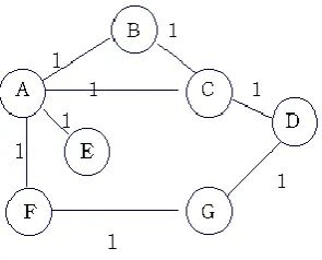
Here it is represented that each node's knowledge about the distances to all other nodes as a table like the one given in Table 1. Note that each node only knows the information in one row of the table.
1. Every node sends a message to its directly connected neighbours containing its personal list of distance. ( for
example, A sends its information to its neighbours B,C,E, and F. )
2. If any of the recipients of the information from A find that A is advertising a path shorter than the one they currently know about, they update their list to give the new path length and note that they should send packets for that destination through A. ( node B learns from A that node E can be reached at a cost of 1; B also knows it can reach A at a cost of 1, so it adds these to get the cost of reaching E by means of A. B records that it can reach E at a cost of 2 by going through A.)
3. After every node has exchanged a few updates with its directly connected neighbours, all nodes will know the
least-cost path to all the other nodes.
4. In addition to updating their list of distances when they receive updates, the nodes need to keep track of which
node told them about the path that they used to calculate the cost, so that they can create their forwarding table. ( for example, B knows that it was A who said " I can reach E in one hop" and so B puts an entry in its table that says " To reach E, use the link to A.)
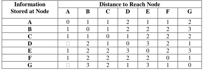
Information Stored at Node
Distance to Reach Node
A B C D E F G
A 0 1 1 2 1 1 2
B 1 0 1 2 2 2 3
C 1 1 0 1 2 2 2
D 2 1 0 3 2 1
E 1 2 2 3 0 2 3
F 1 2 2 2 2 0 1
G 3 2 1 3 1 0
Table 2. final distances stored at each node ( global view).
IV. ANALYSIS USING MATLAB
The coding done for distance vector routing and link state protocol are implemented on MATLAB 7.11 (R2010b) and the system configuration of Intel Core i3- 1.90 GHz with 64 bit operating system. The code finds the shortest path from source to destination node. First it asks for number of nodes, and then it generates a figure of entire network with nodes distributed in space with time delay between nodes. Then it computes the shortest path. The coding for this process has been done on the MATLAB script which is based on Bellman–Ford algorithm and Dijkstra‟s Algorithm respectively. The algorithms have been shown below:
Bellman-Ford Algorithm Dijkstra’s Algorithm
d[s] 0
for each v Î V – {s}
dod[v] ¥
fori 1 to|V| – 1
do for each edge (u, v) Î E do ifd[v] > d[u] + w(u, v)
thend[v] d[u] + w(u, v)
for each edge (u, v) Î E do ifd[v] > d[u] + w(u, v)
thenreport that a negative-weight cycle exists
At the end, d[v] = d(s, v), if no negative-weight cycles. Time = O(VE).
dist[s] ←0 for all v ∈ V–{s}
do dist[v] ←∞
S←∅
Q←V while Q ≠∅
do u ← mindistance(Q,dist)
S←S∪{u}
for all v ∈ neighbors[u] do if dist[v] > dist[u] + w(u, v)
then d[v] ←d[u] + w(u, v)
V. SIMULATION RESULT
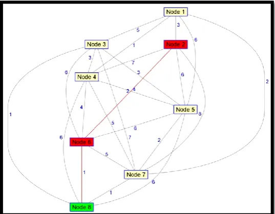
In Link state protocol coding the network of eight nodes is shown above with their intermediate nodal distances and when the shortest distance between source and the destination is calculated by the link state protocol then the results obtained has been shown in figure given below in which source node is „2‟ and the destination node is „8‟ in which the shortest path is calculated with the node „6‟ as an intermediate node.
Figure 3. Shortest path from source to destination node according to Link State Protocol
Figure 4. Layout of entire network of eight nodes
Figure 5. Shortest path between source and destination according to Distance Vector Routing Protocol
Hence with the help of above figures we simulate the both protocols. No doubt, both types of routing protocols have some advantage and disadvantage over each other. In different situation one of both routing protocol can be implemented. In the given table you can find differences between distance vector and link state routing protocol.
DISTANCE VECTOR LINK STATE
Algorithm Bellman-Ford Dijsktra
Network view Topology knowledge from the
neighbour point of view
Common and complete
knowledge of the network
topology
Best Path Calculation Based on fewest number of hops Based on the cost
Updates Full routing table Link State Updates
Updates Frequency Frequently periodic updates Triggered updates
Routing Loops Needs additional procedures to
avoid them
By construction, routing loops cannot happen
CPU and Memory Low utilization Intensive
Simplicity High simplicity Requires a trained network
administrator
Convergence time Moderate Fast
Updates On broadcast On multi cast
Updating contents Whole routing table Only changed information
HOP Limited Unlimited
Hierarical Structure No Yes
Intermediate Nodes No Yes
Table 3. Comparison between distance vector protocols and link state protocols
VI. CONCLUSION & FUTURE SCOPE
protocol shows that distance vector protocols have frequently periodic updates, low utilization of CPU and memory and has high simplicity whereas the link state protocols have intensive utilization of CPU and memory with a high complexity which requires a well trained administrator to be handled. We could work towards improving the algorithm so as to avoid the major evils of this algorithm namely Count to Infinity, Bouncing Effect and Looping. This would help making the algorithm more dynamic and decreasing the amount of time it takes to re-compute the routes.
Routing protocols support the delivery of packets, in spite of changes in network topology and usage patterns, by dynamically configuring the routing tables maintained at routers in internets. The compromise of this routing function in an internet can lead to the denial of network service, the disclosure or modification of sensitive routing information, the disclosure of network traffic or the inaccurate accounting of network resource usage. The future scope of this paper is to focus on security services in routing protocols which is the protection of routing information from threats to the integrity (the intentional corruption of routing data), authenticity (the acceptance of routing information from an unauthorized entity by legitimate routers), and in some cases the confidentiality (of for example sensitive policy information) of routing updates.
REFERENCES
1. Asmaa Shaker Ashoor, “Performance Analysis Between Distance Vector Algorithm (DVA) & Link State Algorithm (LSA) For Routing Network”, IJSTER Volume 4, Issue 02, FEB 2015
2. Sumitha J. “Routing Algorithms in Networks”, Research Journal of Recent Sciences, ISSN 2277-2502 3. Vol. 3(ISC-2013),1-3 (2014)
4. Hanumanthappa. J., Manjaiah D H, “A Study on Contrast and Comparison between Bellman-Ford algorithm and Dijkstra‟s Algorithms” 5. Jin Y. Yen. "An algorithm for Finding Shortest Routes from all Source Nodes to a Given Destination in General Network", Quart. Appl. Math.,
27, 1970, 526-530.
6. Richard Bellman: On a Routing Problem, in Quarterly of Applied Mathematics, 16(1), pp.87-90, 1958. 7. Lestor R. Ford jr., D. R. Fulkerson: Flows in Networks, Princeton University Press, 1962.
8. Thomas H. Cormen, Charles E. Leiserson, Ronald L.Rivest, and Clifford Stein. Introduction to Algorithms, Second Edition. MIT Press and McGraw-Hill, 2001. ISBN 0-262-03293-7. Section 24.1: The Bellman-Ford algorithm, p.588–592. Problem 24-1, pp.614–615.
9. Venkateshwara Rao .K, Dynamic Search Algorithm used in Unstructured Peer- to-Peer Networks, International Journal of Engineering Trends and Technology, 2(3),(2011).
10. Cheolgi Kim, Young-Bae Koy and Nitin H.Vaidya, LinkState Routing Protocol for Multi-Channel Multi-Interface Wireless Networks, IEEE (978–1–4244–2677–5/08)/$25.00c (2008).
11. Kiruthika R., An exploration of count-to-infinity problemin networks” International Journal of Engineering Science and Technology, 2(12), 7155-7159 (2010)
12. Mohammad reza soltan aghaei, A hybrid algorithm for finding shortest path in network routing, Journal of Theoretical and Applied Information Technology © 2005-2009 (2009)
13. Taehwan Cho, A Multi-path Hybrid Routing Algorithm in Network Routing, International Journal of Hybrid Information Technology, 5(3), (2012)
14. Ruchi Gupta, Akhilesh A.Waoo and Dr. Sanjay Sharma, “A Survey of Energy Efficient Location Based Multipath Routing ” in IJCA, Dec 2012.