University of Windsor
University of Windsor
Scholarship at UWindsor
Scholarship at UWindsor
Electronic Theses and Dissertations
Theses, Dissertations, and Major Papers
1-1-2007
Throughput analysis and improvement of paint shop in
Throughput analysis and improvement of paint shop in
automobile industry.
automobile industry.
Guangming Qiu
University of Windsor
Follow this and additional works at:
https://scholar.uwindsor.ca/etd
Recommended Citation
Recommended Citation
Qiu, Guangming, "Throughput analysis and improvement of paint shop in automobile industry." (2007).
Electronic Theses and Dissertations. 7128.
https://scholar.uwindsor.ca/etd/7128
THROUGHPUT ANALYSIS AND IMPROVEMENT OF
PAINT SHOP IN AUTOMOBILE INDUSTRY
By
Guangming Qiu
A Major Paper
Submitted to the Faculty of Graduate Studies and Research
Through Industrial Engineering
In Partial Fulfillment of the Requirements for
the Degree of Master of Applied Science
at the University of Windsor
Windsor, Ontario, Canada
2007
1 * 1
Archives Canada
Library and
Published Heritage
Branch
395 W ellington Street Ottawa ON K 1A 0N 4 Canada
Bibliotheque et
Archives Canada
Direction du
Patrimoine de I'edition
395, rue W ellington Ottawa ON K 1A 0N 4 Canada
Your file Votre reference
ISBN: 978-0-494-42319-6
Our file
Notre reference
ISBN: 978-0-494-42319-6
NOTICE:
The author has granted a non
exclusive license allowing Library
and Archives Canada to reproduce,
publish, archive, preserve, conserve,
communicate to the public by
telecommunication or on the Internet,
loan, distribute and sell theses
worldwide, for commercial or non
commercial purposes, in microform,
paper, electronic and/or any other
formats.
AVIS:
L'auteur a accorde une licence non exclusive
permettant a la Bibliotheque et Archives
Canada de reproduire, publier, archiver,
sauvegarder, conserver, transmettre au public
par telecommunication ou par Nntemet, preter,
distribuer et vendre des theses partout dans
le monde, a des fins commerciales ou autres,
sur support microforme, papier, electronique
et/ou autres formats.
The author retains copyright
ownership and moral rights in
this thesis. Neither the thesis
nor substantial extracts from it
may be printed or otherwise
reproduced without the author's
permission.
L'auteur conserve la propriete du droit d'auteur
et des droits moraux qui protege cette these.
Ni la these ni des extraits substantiels de
celle-ci ne doivent etre imprimes ou autrement
reproduits sans son autorisation.
In compliance with the Canadian
Privacy Act some supporting
forms may have been removed
from this thesis.
While these forms may be included
in the document page count,
Conformement a la loi canadienne
sur la protection de la vie privee,
quelques formulaires secondaires
ont ete enleves de cette these.
ABSTRACT
It is natural that if a thing happens two times under similar conditions, it is likely to get the
same result. Based on this assumption, the simulation model of a paint shop is built by
software AutoMod to generate an artificial history to draw inferences about the operating
characteristics of the real system. This model considers many factors that could affect the
throughput, such as mixed products, optimal buffer location, varying part arriving rate, mean
time between failures, mean time to repair, and maintenance policy. Using simulation as
modelling techniques is a general approach to the complex situation where analytical
DEDICATION
ACKNOWLEDGEMENTS
I feel fortunate to have had a lot of people who helped me completing the program of Master
of Applied Science. I would like to take the opportunity to express my sincere gratitude to Dr.
Walid Abdul-Kader, my academic advisor, for his encouragement, patience, invaluable
advice through the course of writing this major paper.
My gratitude also goes to Dr. R. Lashkari, who acted as my committee member, for the time
he spent reading and examining this major paper. His valuable suggestions helped
significantly improve the quality of my work.
Sincere gratitude is also expressed to the faculty and staff of the Department of Industrial and
Manufacturing Systems Engineering for providing me with such an excellent research
TABLE OF CONTENTS
ABSTRACT
iii
DEDICATION
iv
ACKNOWLEDGEMENTS
v
TABLE OF CONTENTS
vi
LIST OF FIGURES
ix
LIST OF TABLES
x
GLOSSARY
xi
CHAPTER
I.
INTRODUCTION
1
II.
LITERATURE REVIEW
4
2.1
Throughput estimation of the single workstation
4
2.2
Throughput estimation of two workstations in series separated by a buffer
4
2.3
Increasing line’s throughput by system configurations
6
2.4
Contribution of properly locating buffer
8
2.5
Increasing throughput by efficient maintenance policy
9
III.
REVIEW OF PAINT SHOP
10
3.1
Process overview
10
3.2
Layout and facility
10
3.3
Paint shop operation
12
IV.
SIMULATION MODELING
14
4.1
Serial system configuration
14
4.2
Simple hybrid system configuration
15
4.3
Factors to be tested
16
4.4
Simulation tools and notation in simulation code
16
V.
SIMULATION EXPERIMENTS AND RESULTS ANALYSIS
17
5.1
Determining warm-up period
17
•
Simulation results and analysis of experiment I
19
5.2
Serial system configuration versus simple hybrid system configuration 19
•
Introduction of experiment II
20
•
Input data of the serial system configuration
21
•
Simulation results and analysis of the serial system configuration
22
•
Input data of the simple hybrid system configuration
23
•
Simulation results and analysis of simple hybrid system configuration 23
•
Comparison of the serial and the simple hybrid system configurations 25
5.3
Determining optimal number of carriers
26
•
Introduction of experiment III
27
•
Simulation results and analysis of experiment III
27
5.4
Determining optimal buffer location
29
•
Introduction of experiment IV
29
•
Input data of experiment IV
30
•
Simulation results and analysis of experiment IV
31
5.5
Corrective maintenance versus preventive maintenance
33
•
Input data of experiment V
33
•
Simulation results and analysis of experiment V
34
5.6
Final throughput
34
•
Input data of experiment VI
35
•
Simulation results and analysis of experiment VI
35
VI.
CONCLUSION AND FUTURE WORK
37
APPENDIX A: CODE OF SERIAL SYSTEM CONFIGURATION
38
APPENDIX B: CODE OF SIMPLE HYBRID SYSTEM CONFIGURATION
50
APPENDIX C: CODE OF DEFINING OPTIMAL BUFFER LOCATIONS
74
APPENDIX D: EXPERIMENTAL DATA OF THE SERIAL SYSTEM
CONFIGURATION
78
APPENDIX E: EXPERIMENTAL DATA OF THE SIMPLE HYBRID SYSTEM
APPENDIX F: EXPERIMENTAL DATA OF THE EFFECT OF VARYING THE
NUMBER OF CARRIERS ON THROUGHPUT IN SIMPLE HYBRID
SYSTEM CONFIGURATION
82
APPENDIX G: EXPERIMENTAL DATA OF THROUGHPUT OF DIFFERENT BUFFER-
COMBIN ATION S
84
APPENDIX H: EXPERIMENTAL DATA OF FINAL THROUGHPUT PER MONTH OF
THE SIMPLE HYBRID SYSTEM CONFIGURATION
85
REFERENCES
86
LIST OF FIGURES
Figure 1.1: Automobile Manufacturing System
1
Figure 2.1: Two workstations in series separated by a buffer
5
Figure 2.2: System configurations
6
Figure 3.1: Layout of paint shop
11
Figure 3.2: End-shift operation routine
13
Figure 4.1: Flow chart of base model I, serial system configuration
14
Figure 4.2: Flow chart of base model I I , simple hybrid system configuration
15
Figure 5.1: Warm-up period
19
Figure 5.2: The effect of varying the number of product types on throughput in serial system
configuration
22
Figure 5.3: The effect of varying the number of product types on throughput in simple hybrid
system configuration
24
Figure 5.4: Throughput illustration
25
Figure 5.5: The effect of varying the number of carriers on throughput in simple hybrid
system configuration
28
Figure 5.6: Buffer location
29
Figure 5.7: Throughput of different buffer-combinations
31
LIST OF TABLES
Table 5.1: Input data of experiment I
18
Table 5.2: Input data of serial system configuration
21
Table 5.3: workstations’ percent of time on set-up when the number o f product types
increases
23
Table 5.4: Probability of product being blocked
25
Table 5.5: WIP of the simple hybrid and the serial system configurations
26
Table 5.6: Possible combination of two buffers in seven locations
30
Table 5.7: Product’s mix-ratio and cycle times
30
GLOSSARY
Buffer
- is used to store loads on semi-finished product
Mean time between failures (MTBF)
- this is a quantity of time from which an object in
working condition will fail
Mean time to repair (MTTR)
- this is a quantity of time required to repair an object which
is currently offline
Steady-state
- is the limit of a response variable of a simulation model if the simulation
model were run without termination
Transient state
- the period after which steady-state is reached
Corrective maintenance
- occurs when a system accidently fails and is usually driven by
the failure of a component or system
Preventive maintenance
- repair and maintenance of the facilities every certain period
White body storage (WBS)
- is used to store white body before a paint shop
Painted body storage (PBS)
- is used to store painted body after a paint shop
System configurations
- are ways to deploying facilities
CHAPTER I: INTRODUCTION
This paper studies a paint shop in the automobile industry. There are five main shops whose
work is required to produce a car: the stamping shop, the body shop, the paint shop, the trim
and chassis shop and the power train shop. The flow of work from stage to stage is illustrated
in Figure 1.1 (with WBS standing for “white body storage” and PBS for “painted body
storage”).
WBS
PBS
Dealer
The body shop The paint shop
Stamping shop
Power train shop The trim and chassis shop
Figure 1.1: Automobile Manufacturing System
Conway et al. (1988) presented six rules for the optimal buffering of balanced lines with
moderate variability. One of these rules is the bowl phenomenon, which states that buffers
should be allocated evenly among all sites—if possible—with any remaining buffers
allocated symmetrically around the center of the line. Furthermore, Powell and Pyke (1996)
stated that while a bottleneck station tends to draw buffers toward it, the optimal allocation
depends on the location and severity of the bottleneck, as well as the number of buffers
available. Therefore, if we consider the entire automobile manufacturing system as a
production line, the paint shop— located in the middle of said line— is likely to act as a
b o t t l e n e c k .
shop, and painted cars with minor defects are taken off the regular production lines and
moved to the repair area. Painted cars with major defects are directed to the rework loops to
be processed again. Once the repair is finished, they are placed back on the regular line as
soon as an opening occurs.
Multiple product types with a variety of surface areas are often processed in the same
painting line. A car with a larger surface area requires more processing time than one car
with a smaller surface area—facts that prompt varying processing times. Color changing is
another common occurrence in the paint shop, i.e. mixed products. When changing color, a
specific set up time is required for some workstations. For example, the plant must cleanse
the painting apparatus of one paint color before switching to a new color.
In order to save on the investment in the painting facility and increase painting quality at the
same time, jobs can enter the painting booths multiple times. For example, products with
major defects are directed back to particular painting booths to be reprocessed, otherwise
another painting booth must be built to perform the repair function. Therefore, Li (2004)
stated that paint shops tend to be system bottlenecks in many automotive assembly plants due
to the complexity of their tasks. This paper selects a paint shop— starting from WBS and
ending at PBS— as a case study.
This is the first time that the two kinds of system configurations are thoroughly compared in
terms of throughput, and a new equation for predicting optimal buffer location is introduced
in Chapter II and validated in our case study.
The remainder of this major paper is divided into five more chapters. Chapter II presents
analytical solutions to the throughput calculation, as well as their strong points and
limitations. Techniques to improve throughput, such as suitable system configuration,
optimal buffer location and an efficient maintenance policy are also offered.
Chapter III focuses on the paint shop, which consists of a material handling system, various
includes various power and free conveyors and carriers (fixtures or skids) to perform the
transportation, buffer and grouping functions. One of the main problems encountered by
designers is the difficulty of gaining insight into how the number of carriers impacts the
throughput. In addition, random failures and the repair time of the paint booths also affect the
system throughput.
Chapter IV—Simulation Modeling—introduces the primary purpose o f the simulation
modeling techniques, the two base models, the different factors to be tested and the
simulation tools.
Chapter V sets up several experiments to analyze the effect o f different factors on system
performance. A modeller could sense how the number of carriers affects the throughput
based on the experimental results. Buffer location is also an important design factor. The
impact of maintenance on the throughput is addressed as well. Ultimately, the final
throughput is presented when all the suitable techniques are applied to the manufacturing
system.
CHAPTER II: LITERATURE REVIEW
In an effort to gain insight into the throughput estimation for the whole manufacturing system,
several typical modules are presented—including how to analyze single workstation
throughput as well as two workstations in a series, separated by a buffer. Theoretically, the
throughput of a complex manufacturing system could be calculated by decomposing the
complex manufacturing system into many simple templates. Several techniques for
improving throughput are presented later, some of which are applied to our case study.
2.1 Throughput estimation of the single workstation
For the single workstation, Sawyer (1970) gave a well-known relation—see equation 2.1—
for predicting the throughput:
Q = T-
(
2
.
1
)
where:
• C = cycle time (the number of time units per product produced on the line)
• T = useful processing time
• Q = throughput
However, further analysis reveals that this equation is not as simple as it initially appears.
How does the designer calculate useful processing time? For example, given a one year
period, the designer can reduce the time for holidays, for breaks and for repairing or setting
up the facility, but how can they estimate the time for starting the production line and the
time for stopping it—during which the production rate of the manufacturing system is
apparently slowing down? In reality, the designer cannot ignore this issue because the factory
manager encounters it whenever there is shift change. This problem is revisited in Chapter III,
with our research trying to provide a solution according to the paint shop’s special rules.
2.2 Throughput estimation of two workstations in series separated by a buffer
Alden (2002) developed a formula estimating the performance of two workstations in series
flow from Station 1 to Station 2, and are to be processed at each station. To derive equation
2.2, which calculates the throughput in a steady state, Alden (2002) treats the movement of
jobs through the line as a fluid flow.
Buffer
Station 2 Station 1
Figure 2.1: Two workstations in series separated by a buffer
The throughput equation developed for this case is given by
p = S 2x P(w,
w)+
S 2
x
P{d, w
)
(2.2)
where:
•
p -
the average number of jobs produced per time unit
•
S
2=
the speed of station 2, i.e. jobs produced per time unit
•
P(w, w) =
the fraction of time that both stations are processing
•
P(d, w)
= the fraction of time that station 2 is processing, while station 1 is down
•
S 2 = S 2 x r^
TBF^ „
(2.2
a)
MTBF2 +
m t t r2
Based on the research conducted by Alden (2002),
1
P(w, w)
=
and
P(d,w) =
(A, + A2
V(,
. 1
\ + BdlP° / + B d*P° / + 02Po /
+ P0
(/I, +
X
2)
c
B02P
o)
1/
/
+ B02PO/ +
b2
p0/ +
pq/
/ f a + A 2)
/
s x/
s2
/ ui
(2.3)
(2.4)
Xi
= 1/MTBFi (mean failure rate of workstation 1)
jj
-2= I/MTTR
2(mean repair rate of workstation 2)
X
2=
I/MTBF
2(mean failure rate of workstation 2)
6 1
=
Xj/(Xj+ X
2)
(for simplifying the above equation)
O
2= 2 /(2 /+
X
2)
(for simplifying the above equation)
P o = 9 i / ( l + 6/B)
(the probability that the buffer is empty)
Alden’s paper also reveals that Equations 2.3 and 2.4 are based on many assumptions—that
“time between failures” and “time to repair” are exponentially distributed, that the first
station is never starved and the second station is never blocked, and that jobs flow through
the system with zero transit time. With so many assumptions (some of them impossible in a
real-world situation), it is inconvenient to give an analytical solution, even if the
manufacturing system is slightly modified. To remedy this problem, another method is
wanted as the manufacturing system becomes more complex.
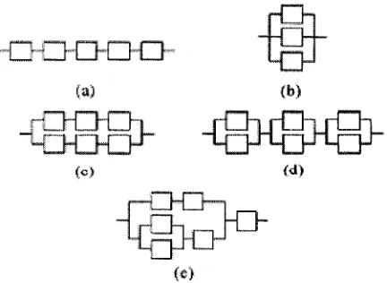
2.3 Increasing line’s throughput by system configurations
Webbink and Hu (2005) stated that the system configuration could be divided into five
categories: (a) serial configuration, (b) parallel configuration, (c) simple hybrid configuration,
(d) complex hybrid configuration and (e) complex-hybrid configuration—as illustrated in
Figure 2.2, where the little rectangle represents a workstation.
MTBF,
MTBR + MTTR,
(b)
These configurations, individually, have their own advantages and disadvantages. For
example, the serial configuration is simple and does not require too many material handling
facilities and the parallel configurations are more reliable. When one workstation breaks
down, the other—possessing the same function—can keep the production line running.
However, parallel configurations demand a complex material handling system and therefore
waste too much time in the process of transportation, which does not add value to the product.
Therefore, a factory manager is faced with a trade-off when selecting a suitable system
configuration.
The studied case in this paper selects the simple hybrid configuration shown in Figure 2.2 (c)
as its strategy for deploying equipment because several kinds of products are mixed together.
Serial configuration requires a particular set-up time when changing product types, leading to
a reduction in the over-all throughput. Furthermore, because most manufacturing systems
now adopt a pull system instead of a push system and the market demand is always varying,
grouping the same products as a batch is sometimes not practical. In this situation, a simple
hybrid configuration could perform the grouping function by the material handling system.
In our case, a “cross-line transportation car” is the material handling equipment used to
convey the first group o f products to the upper serial line and the second group o f products to
the lower serial line (i.e. “grouping”). Both the upper and lower serial lines perform the same
sequence of processes.
In addition, from a reliability standpoint, a simple hybrid configuration is better than a serial
configuration. For example, if one of the workstations in the upper serial line breaks down,
the factory manager can continue to run the production line as a whole by using the lower
serial line. Failures in both the upper and lower serial production lines, however, causes the
production to stop completely.
Chapter V studies and compares the serial configuration and the simple hybrid configuration
2.4 Contribution of properly locating buffer
Powell and Pyke (1996) studied the problem of buffering serial lines with moderate
variability and a single bottleneck—a single station with a larger mean processing time than
all other stations. Their analysis reveals that a bottleneck station draws buffers towards itself,
but the optimal allocation depends on the location and severity of the bottleneck, as well as
the number of buffers available.
In our case, a simple hybrid configuration is adopted as our deploying strategy. A restricted
factory space prompted us to allow two buffers— each with a capacity o f 1—in each line of
the simple hybrid configuration. Therefore, the designer does not worry about the buffer
capacity, only the buffer location. This makes the buffer analysis much easier.
The mean processing time for each workstation in our case is almost the same as the cycle
time. The main difference between the various workstations is their mean time between
failures, and mean time to repair. The spraying guns in the paint booth are very sensitive to
the density of paint material, and frequently become blocked. Therefore, the painting booths
have a much lower mean time between failures.
However, the conclusions, drawn by Powell and Pyke (1996), could be expanded by the
assumption of replacing a larger mean processing time with a slower speed (see Equation 2.2
a) in order to conceptually predict a bottleneck in a serial production line. In addition,
Equation 2.5 expresses the workstation’s parameter for mixed products if the set up time is
ignored.
1
MTBF
S
---x ---
(2.5)
+
n2t2 +•■■ nntn
MTBF + MTTR
Where,
•
n„ =
the number of nth product
Equation 2.5 is used to conceptually predict a serial line’s bottleneck in the simple hybrid
configuration, and is validated by the simulation model. For more information, please refer to
Experiment IV in Chapter V.
2.5 Increasing throughput with efficient maintenance policy
Maintenance activities are performed to enhance or restore efficiency and alleviate the risk of
losing throughput. Zhang (2005) presented that maintenance activities can be categorized as
corrective maintenance (CM) or preventive maintenance (PM). CM occurs when a system
experiences a random failure—usually driven by the failure o f a component or system. PM
occurs when a system can still run and be performed in either a time-based or a condition-
based manner.
The challenge the designer faces is not knowing which maintenance policy is more efficient,
because efficiency depends on the reliability of the components and the system, or the failure
rate curve. In addition, preventive maintenance can only reduce a facility’s failure rate to a
certain level, it cannot effectively prevent accident failures. This makes selecting a suitable
maintenance policy more complex, because the levels depend on the frequency that
preventive maintenance is performed. Chapter V compares data provided by the maintenance
CHAPTER III: PAINT SHOP REVIEW
This chapter introduces the paint shop in our case study, presenting an overview of the paint-
process as well as the layout and operation of the shop.
3.1 Process overview
The white bodies are transported from the automotive body shop to the paint shop, where
they undergo pre-paint treatment. —a process that involves thorough washing and phosphate,
which is used to cause a chemical crystallization on the white body surface that provides
improved paint adhesion and anti-corrosion protection.
The white bodies dry, and are directed through the process of base-coat application—a layer
of material applied to the vehicle surface that causes the top-coat to readily adhere to the
surface of the vehicle. The base-coat material requires excellent adhesion to both the
automotive white body—generally made of lightweight steel— and the top-coat painting
material.
The truck bodies are then transported to a bake oven where the base-coating is cured and
dried, prior to being directed to the sanding booth where the surface o f the base-coat is made
coarser to improve its adhesive ability. Forced cooling is provided by the cooling-booth
between the bake-oven and the sanding-booth to lower the temperature o f the truck bodies to
around 45 °C.
When the top-coating process is finished—one similar to the base-coating process—the
painted bodies undergo inspection and repair in terms of paint quality and correctable defects.
3.2 Layout and facility
As previously stated, the facilities are finally deployed according to a simple hybrid
configuration—illustrated in the conceptual layout of Figure 3.1—where the squares
represent various facilities and the stars signify the candidate buffer locations. Grouping
into a variety of serial production lines. Only two Capacity 1 buffers are allowed in each
parallel production line, due to space limitation and investment-efficiency on the paint shop
floor. The size and shape of the truck bodies—approximately ten meters long and two meters
high whether they are stacked or stored on the same level—the buffer occupies too much
space in the paint shop. Chapter V addresses the optimal buffer location.
1
I
o Jf
Cl,
cd
CL,3
O
5*
h-1
Other workstations—except the phosphate and drying booths— are doubled because the
production rates of the phosphate and drying booths are much faster than the rates of the
other workstations. In addition, the phosphate and dry-up processes are similar even for
different products—unlike other workstations, such as base-coat and top-coat, which must
change the performance of their tasks with the changing product types. The cross-line
transportation car is the material handling equipment used to perform the grouping function.
According to PLC code, it can separate different products and send them to one of the base-
coat booths, based on the “first come first serve” principle.
White truck bodies are only placed on carriers in the loading zone before they are conveyed
to the next process if two conditions have been met. The first is that there are white truck
bodies in the WBS. The second is that carriers are available in the carrier storage. Once the
entire painting process is complete, the truck bodies are transported to the unloading zone
where they separate with the carriers. The workers then put the carriers in the carrier storage,
and the painted bodies in PBS.
3.3 Paint shop operation
The paint shop runs eight hours a day, five days a week. During its daily operation,
production must be scheduled so that end-shift changes can be made with a minimum of
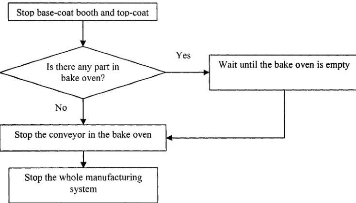
interruption in production. Scheduling the end-shift is difficult because the conveyors
running parts through bake ovens cannot be stopped for long, or they risk inflicting damage
resulting from the high temperature. With this in mind, the manager empties all the bake
ovens before shift, leading to a temporary slow down for the throughput o f the whole system.
The end-shift operation routine is illustrated in Figure 3.2, and this special rule makes the
calculation of useful processing time in Equation 2.1 very complex. Chapter V includes the
shifting impact in the simulation model to accurately estimate the performance o f the whole
system.
To prevent paint build-up on spray gun tips, each paint-delivery hose and spray gun are
purged with solvent between each change in color. Despite these efforts, the spray guns are
booths to suffer a high fraction of down time. Consequently, they test CM and PM to
minimize the impact caused by the facility’s various fractions of down time.
Yes Is there any part in
bake oven?
No
Stop base-coat booth and top-coat
Stop the conveyor in the bake oven
Stop the whole manufacturing system
Wait until the bake oven is empty
CHAPTER IV: SIMULATION MODELING
The first step in designing the simulation model was to identify its primary purpose. In our
case, the primary purpose of simulating the manufacturing system was to estimate the
throughput and test different factors that might increase throughput before the final layout is
applied to the shop floor. Two base models were built to compare serial system configuration
and simple hybrid system configuration. After selecting a suitable system configuration,
different factors with potential effects on the throughput were tested. These factors are the
number of carriers, buffer locations and maintenance policies.
4.1 Serial system configuration
Base Model I was built to estimate the throughput of a serial system configuration, and then
compared with the simple hybrid system configuration estimated by Base Model II. The flow
chart of Base Model I is illustrated as Figure 4.1.
-►I P i o d u c l w a i t s
1‘US
No
Increase one carrier Is carrier
available?
Yes
Is product same
as last one? Unloading
No
Yes
Set up product processing param eter
Oiv up
______
:
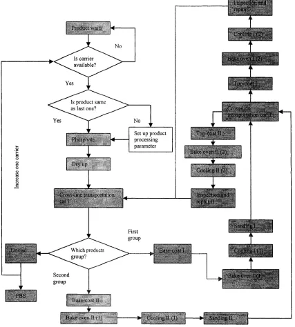
4.2 Simple hybrid system configuration
Base Model II is built to estimate the throughput of a simple hybrid system configuration
and then compared with the serial system configuration estimated by Base Model I. The flow
chart of Base Model II is illustrated in Figure 4.2.
Inspection and | repair 1
1 1'ioduci \v jiu
•d---Is carrier
No
i
Cooliti] U ( 2 )
available?
Is product same
as last one? Cros$*ime
transportation ca t
Set up product processing param eter
Top-coat II
Plursph.Ue
ake oven TI (2)
i ) l s l i p
lo o lin g II (2)
t l O h S - i m e t r j j u p o r u i i o
carl
Inspection and repair Jfi
group
Unload Which products
group?
Uase-coat
Second group
r
1 ’
^jjl Flake oven 1 (1 )
r
Basse-coat 11
♦
, Bake oven 11(1) ► 1 1 >ling I I11) ► Sanding 11
4.3 Factors to be tested
After a suitable system configuration is selected, various factors such as the quantity of
carriers, buffer locations and maintenance policies—all of which have a potential influence
on the final throughput— are tested by the simulation of Base Models I and II.
4.4 Simulation tools and notation in simulation code
The simulation models were built using AutoMod—a commercial simulation package that
combines CAD-like drawing tools with a powerful engineering-oriented language to model
control logic and material flow. Unlike most other simulation languages, AutoMod’s strong
graphical interface precisely captures the physical constraints of distance, size and space-—
producing exceptionally accurate 3-dimensional details.
To help readers understand the simulation code, a summary of the notation is presented
below:
• V l_ ... = variable used for product 1
• V2_... = variable used for product 2
• V3_... = variable used for product 3
• V4_... = variable used for product 4
• V5_... = variable used for product 5
• V 6_... = variable used for product 6 • V7_... = variable used for product 7
• V8_... = variable used for product 8
• V_... = variable used for all products
• A ... = load attribute
• R_... = resource
• P_— = process
• L_... = load
• C o n v = p o w e r a n d fre e c o n v e y o r sy s te m
• Pm = automatic guided vehicle system
• Sta_... = workstations
• Lbl_... = labels
CHAPTER V: SIMULATION EXPERIMENTS AND RESULTS ANALYSIS
Chapter V is divided into six sections. The first section defines the warm-up period using a
leading base model, then applies the warm-up period and the steady-state length to the
subsequent simulation models. The second section compares the simple hybrid system
configuration with the serial system configuration in terms of throughput when the number of
product types varies. The third section determines the optimal number o f carriers. The fourth
section uses a conceptual simulation model to validate Equation 2.5, which predicts the
optimal buffer location. The result is then applied to arrange the facilities on the shop floor.
The fifth section addresses factory management—with the maintenance policies considered
in this experimental design. The last section predicts the throughput per month when the end-
shift change is considered.
5.1 Determining warm-up period
Most of the simulation models are started empty and idle. Almost every time, these
conditions differ from the steady-state condition. Therefore, the simulation model takes some
time to reach steady-state. During this time period, the model is said to be in transient-state,
i.e. warming up.
Mahajan and Ingalls (2004) categorized the methods for dividing the warm-up period into (1)
graphical, (2) statistical, (3) heuristics and (4) initialization bias methods. In this paper, the
graphical method is employed to define the warm up period using a leading base model. All
the following experiments are analyzed with data recorded from the simulation steady-state
behavior.
• Introduction of Experiment I
The leading base model is designed to define the warm-up period. Eight kinds of products are
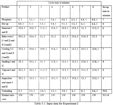
• Input data for Experiment I
Table 5.1 presents the input data for Experiment I. Column 1 reports the name of different
workstations. In the table, all the cycle times are the uniform distribution. And the first value
is the mean o f the distribution, while the second value is the standard deviation.
By
using
uniform distribution, the maximum and minimum processing times are limited that accords
to the reality.
Cycle time in minutes
Product 1 2 3 4 5 6 7 8 Set-up
time in
minutes
Phosphate 5, 1 5.2, 1 5.5, 1 5.6, 1 6.0, 1 6.2, 1 6.4, 1 6.6, 1 7
Dry up 4.8, 1 5, 1 5.2, 1 5.4, 1 5.5, 1 5.5, 1 6 ,1 6.4, 1 8
Basecoat I
and II
10.4,3 10.6,3 11.2,3 12.4,3 12.6,3 12.8,3 13,3 13.2,3 6
Bake oven I
(1 and 2) and
II (land2)
10.2,2 10.4,2 11,2 12,2 12.3,2 12.6, 2 12.8,2 1 3 ,2 6
Cooling 1(1
and 2) and II
(land2)
10.2, 1 10.4, 1 10.9, 1 11.8, 1 12.4, 1 12.7, 1 12.7, 1 12.9, 1 7
Sanding I and
II
10, 1 10.2, 1 11, 1 11.8, 1 12.3, 1 12.5, 1 12.8, 1 12.8, 1 8
Topcoat I and
II
10.3,3 10.5, 3 11.3,3 12.3,3 12.5,3 12.8,3 13.1,3 13.4,3 8
Inspection
and repair I
and II
10.1, 1 10.3, 1 11.1, 1 12.1, 1 12.2, 1 12.6, 1 13, 1 13.2, 1 6
Unloading 5 ,1 5.1, 1 5.4, 1 5.3, 1 5.8, 1 6 ,1 6, 1 6.6, 1 N /A
Product
mix-ratio
1/N 1/N 1/N 1/N 1/N 1/N 1/N 1/N N :l~ 8
• Simulation results and analysis of Experiment I
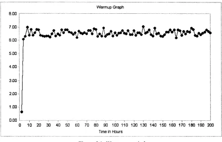
Figure 5.1 is based on the data from Experiment I. The X-axis in Figure 5.1 represents the
time in hours, while the Y-axis tells us the throughput per hour. Figure 5.1 suggests that the
manufacturing system enters the stable-state after 20 hours.
For the sake of insurance, the warm-up period is enlarged to 50 hours, and the simulation
model is run for 1000 hours after the first 50 hours. During these 1000 hours, the simulation
data are collected and analyzed to compare serial system configuration with simple hybrid
system configuration and determine the optimal number o f carriers, predict the optimal
buffer locations and choose a suitable operation policy.
Warmup Graph 8.00
7.00
6.00
5.00
4.00
3.00
2.00
1.00
0.00
0 10 20 30 40 50 60 70 80 90 100 110 120 130 140 150 160 170 180 190 200
Time in Hours
Figure 5.1: Warm-up period
5.2 Serial system configuration versus simple hybrid system configuration
The first step in designing a manufacturing production line is to choose a strategy for
Which system configuration the designer finally chooses depends on a variety o f restrictions.
For example, if the truck paint shop floor is long and narrow, a serial system configuration is
a better choice because the final shape of a serial system configuration on the shop floor
usually appears as a slot that maximizes the floor’s utilization.
Another important restriction is the investment. More capital expenditure means a highly-
automated manufacturing system where a central control room could be set up to supervise
and direct the material flow. This would allow the cross-line transportation cars to distinguish
different products and convey them to the appropriate serial production lines according to
PLC code, i.e. grouping.
There are two major benefits of grouping. The first is that it basically balances the different
production lines according to the products’ cycle times. For example, there are four types of
products produced in two identical production lines. The cycle times o f the four types of
products are 4.2, 6.3, 8.5 and 10.6 minutes, separately. The material handling system can
group the products that have 4.2 and 10.6 minute cycle times together in one production line,
and the other two products into another production line—resulting in two balanced
production lines with near 14.8-minute cycles. The other benefit is that it saves set-up time,
as mentioned in Section 2.2.
• Introduction of Experiment II
The product goes through the same kind of process whether it’s in the serial or simple hybrid
system configurations. However, except for the phosphate, dry-up and unloading
workstations, the number of other workstations in the simple hybrid system configuration are
doubled when compared with the serial system configuration— as illustrated in Figures 4.1
and 4.2. As a result, the production rate of the workstations in the simple hybrid system
configuration should be twice as slow as the production rate in the serial system
configuration. Apparently the equipment with a fast production rate is generally more
set-up times for the workstation in the serial system configuration are also doubled, when
compared with the simple hybrid system configurations— as illustrated in Tables 5.2 and 5.4.
This paper selects a suitable system configuration based on throughput. Two separate
simulation models are built to predict the throughputs of the serial and the simple hybrid
system configurations, according to a certain number of product types. At this level, the
modeller does not need to consider the impact that the quantity of carriers, buffer location,
random failures and maintenance policies have on the throughput— a fact that dramatically
simplifies the simulation models.
• Input data for the serial system configuration
Table 5.2 represents the cycle times of different products in different workstations in minutes.
All the cycle times are uniform distribution. For example, the cycle time of Product 4 at the
phosphate workstation is an uniform distribution with a mean of 5.6 and a standard deviation
o f l .
Cycle time in minutes
Product 1 2 3 4 5 6 7 8 Set-up time
in minutes
Phosphate 5 ,1 5.2, 1 5.5, 1 5.6, 1 6.0, 1 6.2, 1 6.4, 1 6.6, 1 7
Dry up 4.8, 1 5 ,1 5.2, 1 5.4, 1 5.5, 1 5.5, 1 6 ,1 6.4, 1 8
Basecoat 5 .2 ,3 5.3, 3 5 .6 ,3 6.2 ,3 6.3 ,3 6 .4 ,3 6 .5 ,3 6 .6 ,3 12
Bake oven
1 and 2
5 .1 ,2 5.2, 2 5 .5 ,2 6 ,2 6.1 5 ,2 6 .3 ,2 6 .4 ,2 6 .5 ,2 12
Cooling 1
and 2
5.1,1 5.2, 1 5.45, 1 5.9, 1 6.2, 1 6.35, 1 6.35, 1 6.45, 1 14
Sanding 5, 1 5.1, 1 5.5, 1 5.9, 1 6.15, 1 6.25, 1 6.4, 1 6.4, 1 16
Topcoat 5.15,3 5.25,3 5.65,3 6.15, 3 6.25,3 6.4, 3 6 .5 5 ,3 6 .7 ,3 16
In s p e c tio n
and repair
5.05, 1 5.15, 1 5.55, 1 6.05, 1 6.1, 1 6.3, 1 6.5, 1 6.6, 1 12
Unloading 5 ,1 5.1, 1 5.4, 1 5.3, 1 5.8, 1 6 ,1 6 ,1 6.6, 1 N/A
• Simulation results and analysis of the serial system configuration
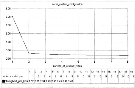
Figure 5.2 is drawn according to the simulation result explicitly in an effort to analyze it. For
the experimental data details, refer to Appendix D, where eighty runs are performed. For
each number of product types, ten replications are performed to get the statistical average
throughput per hour. There are eight types of product, in total, to be tested in the
manufacturing system. Therefore, eighty runs are performed. In Figure 5.2, the X-axis
represents the number of product types, while the Y-axis indicates the throughput per hour.
serial_system_canflguration
7.00
600
5.00
s
4.00
3.00
2.00
I
1 2 3 4 5n ,jm be r_o I _or oduci _ty pc:
6 7 8
1 3 4 i5 6 7 !8 9 10 11 12 13 14 (15 116 117 18
... ■
■
.
\
1
|
|...
number of product types 1: 2 \ 3: 4j 5 6 7; 8 ft fl 0 0 0 Oj
o|
0o!
0■
...
. . .
. ...
.
I ....|.~... ■}
I...
B throughput _per_hOLJi 7 07 2 67 2 54 2.49 2 45 2 43 2 42 2.40 | j ) | 19
Figure 5.2: The effect of varying the number of product types on throughput in serial system
configuration
It is reasonable to state that the throughput decreases as the product type increases, due to the
time spent on set-up. When there is only one type of product, no set-up is needed and the
percentage of time spent on set-up is zero, as illustrated in Table 5.3. As the number of
product types increases to two, workstations require set-up whenever there is a product
a particular number. Table 5.3 also reveals that the percentage of time spent on set-up only
gently increases when the types of products increases from two to three, three to four, four to
five, five to six, six to seven and seven to eight. Take the phosphate workstation as an
example. When the number of product types changes from one to two, the percentage of time
spent on set-up increases 15.5-0=15.5. When the number of product types changes from two
to three, the percentage of time spent on set-up increases 19.9-15.5=4.4. Following this
routine provides the numbers 1.9, 1.2, 0.9, 0.1, and 0.8. As 15.5 is much bigger than 1.9, 1.2,
0.9, 0.1 and 0.8, the throughput dramatically reduces from 7.07 to 2.67 when the number of
product types changes from one to two, and drops down slightly as the number of product
types changes further.
Percentage o f time spent on set-up
The number o f product types 1 2 3 4 5 6 7 8
Phosphate 0 15.5 19.9 21.8 23 23.9 24 24.8
Dry up 0 17.7 22.5 24.8 26 27.1 27.8 28
Base-coat 0 26.6 33.9 37.2 39.2 40.5 41.4 42.1
Bake oven land2 0 26.6 33.9 37.2 39.2 40.5 41.5 42.1
Cooling land2 0 30.9 39.5 43.2 45.8 47.5 48.2 49.3
Sanding 0 35.5 45.1 49.3 52.2 54.2 55.2 56.3
Top-coat 0 35.5 45.1 49.3 52.2 54.2 55.2 56.3
Inspection and repair 0 26.6 34 37.2 39.2 40.5 41.4 42.1
Table 5.3: Workstations’ percentage of time spent on set-up when the number o
types increases
product
• Input data for the simple hybrid system configuration
The input data are the same as the data in figure 5.1. The product mix-ratios are the same for
all kinds of product.
•
Simulation results and analysis of the simple hybrid system configuration
Figure 5.3 is drawn based on the simple hybrid system configuration. For experimental data
One might ask why the throughput drops down dramatically for the simple hybrid system
configuration when the number of product types changes from one to two? We know that no
set-up is needed when two types of products are produced by the simple hybrid system
configuration.
s imp le _h y b rid _s y ste m _c on tig urat i on
throughputjoerjiour
3 4 5 6
I number _o1joroducts
i 1 2 13 14 IS IS 17 IS 19 10 111 112 (13 14
I n u m b e r of p r o d u c t types 11 2 j 3; 4i 5* 6i 7 1 8; 0: 0 i Oi 0 | 0 | 0
— throughput_per_hour 6.20 4 31 3 6 8 3.69 3 50 !3 50S3 38 3 38
15 16 17 | l8 |l 9 D 0
___
oj o | CFigure 5.3: The effect of varying the number of product types on throughput in simple hybrid
system configuration
Figure 5.4 presents an answer to this question, with the rectangles representing workstations
and the circles signifying loads. When there is only one type of product, the products are
directed to the upper and lower serial lines one-by-one. When there are two types of products,
the first type of product is conveyed to the upper serial line and the second type of product to
the lower serial line to save set-up time, i.e. grouping products. In addition, the loads arrive
randomly, so the same kind of product is sometimes grouped together, leading to the
increasing probability that either the upper or lower serial lines will become blocked when
the number o f product types changes from one to two. Therefore, the throughput decreases
0 © O G)
W orkstation 1-2
W orkstation 1-1 W orkstation 1-3
W orkstation 2-1 W orkstation 2-2 W orkstation 2-3
Figure 5.4: Throughput illustration
The above analysis is also verified by the simulation data in Table 5.4, which shows the
probability of the product being blocked in the dry-up workstation (before Workstations 1-1
and 2-1) when the processing is over. As the number of product types changes from one to
two, the probability of the product becoming blocked increases from 0.39 to 0.55, leading to
a decrease in throughput.
The number o f product types 1 2
Probability o f product being blocked 0.39 0.55
Standard deviation 0.03 0.02
Minimum 0.34 0.53
Maximum 0.43 0.60
Median 0.39 0.54
Number o f runs 10 10
Table 5.4: Probability of product becoming blocked
• Comparison of the serial and the simple hybrid system configurations
Figures 5.2 and 5.3 tell us that the throughput of the serial system configuration for one type
of product is 7.07 per hour, while the throughput of the simple hybrid system configuration
for the same product is 6.20 per hour. Therefore, the serial system configuration performs
better than the simple hybrid system configuration for one type of product. The simple hybrid
system configuration needs a complex material handling system (cross-line transportation
cars), which leads to spending more time on work-in-process (W1P) than the serial system
configuration. The simulation data from Table 5.5 also shows that the product spends more
The simple hybrid system configuration The serial system configuration
Average 43.8 minutes 38.7 minutes
Standard deviation 0.2 minutes 0.1 minutes
Minimum 43.6 minutes 38.5 minutes
Maximum 44.1 minutes 38.9 minutes
Median 43.9 minutes 38.8 minutes
Number o f runs 10 10
Table 5.5: WIP of the simple hybrid and the serial system configurations
As the product type increases from one to two, however, a significant difference occurs
between the two kinds of system configurations. The throughput of the simple hybrid system
configuration is around 4.31 per hour—much higher than the throughput of the serial system
configuration, which is approximately 2.67 per hour. When the number of product types
increases further, the modeller finds that the curve of the simple hybrid system configuration
is always above the curve of the serial system configuration.
Analyzing both types of system configurations allows one to choose a suitable strategy for
deploying facilities in terms of throughput. In the paint shop, different products are often
produced together, and comparing the two sets of data reveals to the designer that the simple
hybrid system configuration is preferred over the serial system configuration because the
number of product types often exceeds one.
5.3 Determining optimal number of carriers
Carriers (a part of the material handling system introduced later) used in the truck paint shop
are also conveyed to some workstations located in the body shop and the trim and chassis
shop. Here, carriers are used to connect different material handling systems in the body shop,
the paint shop and the trim and chassis shop.
Graehl (1992) stated that simulation studies of large material handling systems include only a
portion of the entire system. One reason for this is that large systems tend to require equally
large and time-consuming simulation efforts. As a result, the modeller defines the scope of
assumes that the carriers are then freed and returned to the carrier storage once the load
arrives at the painted body storage. Another assumption is that one kind of carrier is designed
to fit all kinds of products. In this way, the designer can gain insight into how many carriers
the truck paint shop needs.
It is important to determine what is a suitable number of carriers. On the one hand, if the
number of carriers is not enough it becomes a bottleneck in the whole manufacturing
system—leading to reduced throughput in the truck paint shop. On the other hand, because
the carriers are bulky and require a lot of space for storage, it is impossible to put many
carriers in the carrier storage— a waste of money and space on the shop floor.
• Introduction of Experiment III
Carriers are used to transport truck bodies from one workstation in the paint shop to another.
Each carrier in this paint shop is able to carry one truck body at a time. The carriers wait in
storage until a white truck body arrives at the white body storage. In the loading zone, the
white truck body is put on top of one carrier, which then goes through all the necessary
processes with the truck body. When said processes are finished, the carrier separates from
the truck body and is conveyed to carrier storage.
Similarly, at this level in the simulation model, the designer excludes optimal buffer location,
shift-changing and maintenance policies as factors with the potential to affect the throughput
in the truck paint shop. The simulation model of the simple hybrid system is furthered by
considering the number of carriers as a factor that affects the throughput—based on the
results from Experiment II. Eighty kinds of product are produced in this case—prompting the
input data to be the same as that in Table 5.1.
• S i m u l a t i o n r e s u l t s a n d a n a l y s i s o f E x p e r i m e n t I I I
Figure 5.5 is obtained by running the furthered model. For more information on the
number_of_carriers
7.00
i.00-5 .0 0 4
4.00
3.00
2.00
! the number of carriers
| throughput _ p e r Jiqui 2.032 2 8 12 51 [2 72 2 93 [3.09 [3.233.32133813.39 3.3813.36 !3.38 '3.38 (3.3813.30 3 .3813.38[3.38 3.33:3 33:3 38 3.383.38
Figure 5.5: The effect of varying the number of carriers on throughput in simple hybrid
system configuration
Figure 5.5 reveals how the throughput dramatically increases with the number of carriers at
the beginning, because there are not enough number of carriers in the whole manufacturing
system. Therefore, a small change in the quantity of carriers prompts a large difference in
terms of throughput. When the number reaches forteen carriers, the throughput gently rises
with the number of carriers until it hits seventeen—at which point the simulation model
enters a stable state and the throughput stops increasing with the number of carriers. It comes
down to a trade-off for the designer. If the efficient utilization of the shop floor is more
important than the little difference in terms of throughput when the number of carriers is
forteen to seventeen, then forteen carriers is preferable to seventeen carriers. Otherwise,
seventeen carriers is preferable. Finally, the designer decides to put seventeen carriers in the
carrier storage.
In addition, the modeller notices that the throughput at seventeen carriers in Figure 5.5 is
3.38— the same as 3.38, the throughput in Figure 5.3 for eight types of product. The
experimental data in Figure 5.3 is obtained by assuming that there are infinite carriers
manufacturing system. Furthermore, when the quantity of carriers reaches seventeen, they no
longer act as the system bottleneck anymore—according to Figure 5.5. Consequently, the
two throughputs are the same.
5.4 Determining optimal buffer location
This section is designed to validate Equation 2.5, which states that the workstation with a
slower parameter draws the buffer towards it (where the parameter is expressed by Equation
2.5). The obtained result is applied in our case study to predict the optimal buffer location in
the simple hybrid system configuration.
• Introduction of Experiment IV
Experiment IV considers cycle times, mean time between failures, mean time to repair and
the product’s mix-ratio as potential factors to define a buffer location. A simulation model
consisting of eight workstations and two buffers is set up to obtain analysis data. Four kinds
of products are produced in this serial production line.
Sanding
Top-coat C ooling 2
C ooling 1 B ase-coat B ake oven 1
B ake oven 2 Inspection and repair
Figure 5.6: Buffer location
F i g u r e 5 . 6 i l l u s t r a t e s t h e c o n f i g u r a t i o n , w i t h t h e r e c t a n g l e s r e p r e s e n t i n g w o r k s t a t i o n s a n d t h e