Integrals over the triplet distribution function without the triplet distribution function

This article was downloaded by: [North Carolina State University] On: 29 September 2011, At: 07:35

Publisher: Taylor & Francis

Informa Ltd Registered in England and Wales Registered Number: 1072954 Registered office: Mortimer House, 37-41 Mortimer Street, London W1T 3JH, UK

Molecular Physics

Publication details, including instructions for authors and subscription information:

http://www.tandfonline.com/loi/tmph20

Integrals over the triplet

distribution function without the

triplet distribution function

F. Lado a a

Department of Physics, North Carolina State University, Raleigh, North Carolina, 27695-8202, U.S.A.

Available online: 22 Aug 2006

To cite this article: F. Lado (1991): Integrals over the triplet distribution function without the triplet distribution function, Molecular Physics, 72:6, 1387-1395

To link to this article: http://dx.doi.org/10.1080/00268979100100971

PLEASE SCROLL DOWN FOR ARTICLE

Full terms and conditions of use: http://www.tandfonline.com/page/terms-and-conditions

Integrals over the triplet distribution function without the triplet

distribution function

by F. L A D O

Department o f Physics, N o r t h Carolina State University, Raleigh, N o r t h Carolina 27695-8202, U.S.A.

(Received 10 October 1990; accepted 13 November 1990)

While the triplet distribution function of disordered systems appears in a wide variety of problems in statistical mechanics, it does so always under an integral sign. In this paper, we propose a new method of evaluating such integrals that involves only pair functions throughout and avoids altogether the need for any explicit representation of the little-known triplet function. The procedure is based on an extension of integral equation theory of classical fluids. Numerical illustrations of the method are given for integrals that arise in the calculation of moments of a local field distribution.

1. Introduction

The need to evaluate integrals o f the form

f d r 3 t~(rls)g (3) (r12 , r13), (1)

where g(3)(rl2 , rl3) is the equilibrium triplet distribution function of a disordered system and ~,(r) is arbitrary, arises in a wide range o f applications in statistical mechanics. There is still no reliable way of computing the triplet function for dense systems, thus the evaluation of such integrals has been carried out by approximating g(S), with unpredictable effects on accuracy, using most often the Kirkwood super- position approximation or else the Feenberg convolution approximation [1]. In this paper, we present a new method that involves only pair functions throughout and avoids altogether the need for any explicit representation of the triplet distribution function.

The problem is first set up as a generalization o f the Kirkwood integral equation [2]. Consider a fluid o f N molecules in a volume V subject to a temperature T, and let tp(r) be the intermolecular potential. We adopt the usual definition of the nth-order distribution function [2],

= N! f

g(")(rl, . 9 9 , r , ) p " Z ~ ( N - n)! dr,+l . . . dru exp ( - - f l U u ) , (2)

where

Z u = f drt 9 9 9 d r s exp ( - f l U x )

is the canonical partition function,

I<~i<j<~N

0026-8976/91 $3.00 ~" 1991 Taylor & Francis Ltd

(3)

(4)

1388 F. Lado

the internal energy, and p = N / V , fl = (kB T ) - J . Now single out, say, molecule 1 and assign to it an additional interaction potential ~k(rlj)/fl with moleculesj = 2, . . . , N, at coupling strength ~; that is, the new internal energy is

N

u,,(~) = u,, + r X r

(5)

j = 2

The obvious generalization o f (2) is then

g(')(rl . . . r~l~) = p ~ Z N ( ~ ) ( N -- n)! dr.+, . . . drN exp (--flUN(O), (6)

with

ZN(r = f dr, . . . drN exp (-- rUN(?,)). (7)

Setting ~ = 0 o f course reduces the generalized functions (6) to the usual versions, (2). We now proceed as for the Kirkwood integral equation [2], differentiating g(2)(r,, r21 0 with respect to ~ to obtain

dg (2) (r,, r 2 ] ~) r

dr - ~J(rl2)g(2)(rl' rE I~) - p ~ dr3 ~(r13) [gtS)(rl, r2, r31 ~)

- g(2)(r,, r21 r r31 ~)]- (8)

For a homogeneous system, the distribution functions will depend only on separation vectors rij = rj - ri; in addition, for spherically symmetric potential tp(r) the descrip- tion o f the ordinary fluid depends on just the magnitudes r~j. Then, dropping the superscript for the pair distribution function (PDF) and setting ~ = 0, we obtain from (8)

g'(rl210) -- dg(rl21 ~) d~ r

- ~b(r,2)g(rl2) -- p f d r 3 ~b(rl3) [gl3)(r,2, r,3) -- g(rl2)g(r,3)]. (9)

With this equation, an integral of the form (1) can evidently be determined from a knowledge of the usual P D F g(r) and of the new pair function g'(r 10) defined in (9). Successful theories are available to determine g(r) from the pair potential ~o(r) [3-8]. We shall be concerned here with obtaining the new function g'(rl 0) to complete the recipe and so bypass the need to know gO). In the sequel, we shall further assume for simplicity that ~k(r) too is spherically symmetric, though the more general case of orientation-dependent ~k(r) can also be accommodated.

2. Calculation ofg'(r]O)

Equation (6) describes a two-component system, in which molecule 1 interacts with the others though the total potential ~(r) + ~k(r)/fl while the remaining N -- 1

molecules interact among themselves through tp(r) alone. The Ornstein-Zernike equations [8] for a two-component mixture in which one component is at infinite dilution are

h(r) - g(r) - 1 = C(r) + p f dr' h(r')C (Ir r'l), (10) ./

(.

h(r

g(r

I - ~ -- C ( r l ~) + p J d r ' h(r'l OC(Ir - r'l). ( l l )

Here

C(r)

is the usual direct correlation function (DCF) for the solvent fluid with intermolecular potential ~o(r) and C ( r l O is the corresponding D C F for the solute molecule. These equations for h and C are complemented with the so-called closure relations [8]

g(r)

= exp [-]~o(r) +

h(r) - C(r) +

B(r)], (12)

g(rl~) = exp [-/~o(r) - ~k(r) + h(rl~) - C(rl~) + B(rl~)], (13)

which introduce the solvent and solute bridge functions,

B(r)

and

B(rl ~),

respectively. Though formally defined by infinite series, these functions in practice must be approximated; the different closures in use today [3-8] stem from different approxi- mations to the bridge function.

Equations (10) and (12), with some expression for

B(r),

are the standard fare of liquid state theory. We shall focus here on (11) and (13) in seeking

g'(rl

0). We first rewrite these equations by eliminating h in favour of the series function S = h - C and deconvoluting (11) using Fourier transforms. The result is

C(rl~)

= exp [-flop(r) - ~k(r) + S(rlr + B(rl~)] - 1 - S(rl~), (14)

S(kl4) =

ph(k)~(kl~),

(15)

where the tilde denotes Fourier transform. Now differentiate with respect to ~ and set = 0 to obtain

C'(rl0) =

g(r)[-~k(r) +

S'(rl0) + B'(rl0)] -

S'(rrO),

(16)

g ' ( k l 0 ) =

pFffk)C'(klO).

(17)

Once B'(rl0) is modelled in some appropriate way (see below), these coupled equations can be solved for S'(rl 0) and C'(rl 0), yielding finally the desired

g'(rl0) =

g(r)[-~k(r) + S'(rlO) +

B'(rl0)]. (18)

This supplies the final ingredient needed in (9) to compute an integral over g~3) using only pair functions.

The final point to be addressed is the modelling of B'(r I 0) in (16) and (18). This question has a natural answer in the context of the optimized reference hypernetted chain ( R H N C ) equation [9-1 l], in which

B(r I ~)

is modelled by the bridge function of a hard sphere fluid,

B(rl~) = BHs(r; a(~)), (19)

where the hard sphere diameter a(~) is varied to minimize the free energy. Since a is the variable that changes with ~, we obtain within the same approximation

dB.s(r; o) ( d ln_a(~)~ (20)

B'(rl0) = o do de }r

The slope of In a(~) is obtained numerically by further solving (14) and (15), within the same framework of the optimized R H N C equation, at small values of ~, including r = 0, the neat fluid.

Equations (16) and (17), which are

exact,

along with the modelled B'(r I 0) of (20), which follows from the successful R H N C closure, constitute the algorithm that

1390 F. Lado

replaces approximations t o gO) for purposes of integrals such as (1). In the next section we illustrate the application of this algorithm for two cases.

3. M o m e n t s o f a distribution

A common instance in which integrals o v e r g(3) (as well as higher distributions) make an appearance is the calculation of moments. These include frequency moments (also called sum rules) for time correlation functions [12, 13], microstructural moments in two-phase random media [14-16], potential energy moments for ther- modynamic derivatives [17], and moments of a local field distribution [I 8, 19]. In the first two cases, the resulting function ~O(r) is orientation dependent, requiring a generalization of the simple algorithm described in w 2 along the lines of the electric microfield calculation [20], and will not be dealt with here. The case of thermodynamic derivatives falls within the scope of w 2 but limits ~O(r) to just the intermolecular potential. For present purposes of illustration, we shall cast the discussion in the language of the local field distribution, which affords more variety in r

A local field arises at a test particle, say molecule 1, when tile particle is subject to a scalar field ~(rlj) from each of the remainingj --= 2, 3 . . . N molecules of a fluid. The field function q~(r) is essentially arbitrary and does not affect the fluid configurations. The net field strength ~experienced by the test particle is a random variable of fluid configuration whose distribution is defined by

P ( ~ ) = ( 6 [ ~ - j ~ = 2 ~ ( r u ) ] l , (21)

where the angle brackets denote an equilibrium average with the Boltzmann factor of (2) to (4).

The calculational awkwardness of the Dirac delta function in (21) is avoided by dealing rather with the Fourier transform of p(~u); writing the delta function in Fourier representation, we obtain

P ( ~ ' ) = ~ dK exp (iK~P) P(K), (22)

where then

P ( K ) =

The moments of the distribution,

l e x p ( - i K j ~ z r 9 (23)

where

m. = r . (26)

J

Explicitly, the first and second moments are

ml = p f dr ~(r)g(r), (27)

3

m. = f ~ d ~ P ~ P ( t P ) , (24)

are then generated by the expansion of the exponential in (23),

1 i

-P(K) = 1 - im, K - ~.. m2 K2 + ~ m3 K3 + . . . , (25)

r

m2 = p J dr ~2(r)g(r)

+ ,0 2 J dr2dr3 ~ J ( r l 2 ) ~ l ( r l s ) g O ) ( r l 2 , r13 ), (28)

where we have used (2). From these, the second central moment is given by

C 2 = m 2 - - m ~

= p f d r d/2(r)g(r)

+ pZ f d r 2 d r 3 ~(r12)~b(r13)[gO)(r12 '

r13) --

g(rl2)g(rl3)].

(29)

The computation of the first and second moments is of particular importance when it is known that P ( T ) is approximately Gaussian.

Direct evaluation of (29) obviously requires an approximation to gt3). From (9), we see that c2 may also be written as

c2 = - p .f dr ~(r)g'(r[O),

(30)

avoiding the need for the triplet correlation function when the pair function

g'(rl O)

is computed instead. The reduction from a three-particle integration in (29) to a simple pair expression in (30) is in itself of computational consequence, quite aside from the accuracy of possible approximations to g(3).

We note in passing that (30) can be generalized to all cumulants c,, defined by

d" In Z(~) ~=0 (31)

c, = (-- 1)" de" '

so that, e.g.,

c 3 = m3 - 3m~mz +

2rn~; the calculation of c3 requires knowledge of the two-, three-, and four-particle correlation functions. From (7), however, we have

d In Z(~) ~'

dr

-

p J dr ~b(r)g(r[ ~),

(32)

so that

c, = p f d r qJ(r)(-1)" ' d"-' g(r[ O (33)

-OU

:=0'

which involves only pair functions. It may, however, prove impractical to extend the technique of w 2 for

g'(r

] 0) to higher derivatives of

g(r I ~).

N o attempt has been made in this direction.

A common expedient for dealing with g~3) in the direct evaluation of (29) or (9) is to invoke the Kirkwood superposition approximation [2],

g(3)(rt2,

rl3 ) ~ g(r12)g(r13)g(r23),

(34)

which leads to

g~A(rl210) =

- g ( r , 2 ) ( ~ ( r , 2 ) + p f d r a ~ ( r , 3 ) g ( r , 3 ) h ( r 3 z ) ) .

(35)

The convolution integral in (35) can easily be evaluated using Fourier transforms. Our purpose now is to compute

g'(rl

0), and from it c2, using the extended R H N C technique of w 2, as well as the superposition approximation for comparison, for two local field distributions: (a) a Lennard-Jones (L J) field,

~b(r) = 4[(a/r) 12

- (o'/r)6], (36)

1392 F. Lado

v

- 7 :

- - 3

- - 4 ~ I

I - . 5

i I

r / o "

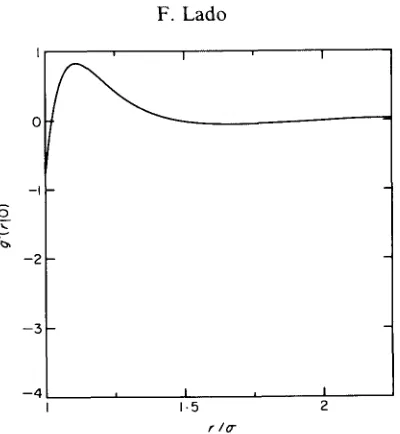
Figure 1. The pair function g'(rl0) of (9) for a Lennard-Jones ~O(r) at a hard sphere test particle in a hard sphere fluid at density p O "3 = 0'4. Integral equation and superposition

approximation results are not clearly distinguishable on this scale.

in a

hardsphere

fluid [18], where the hard sphere diameter is also a so the test sphere experiences only the attractive part o f ~b(r); and (b) a C o u l o m b field

e 2

~k(r) = - - (37)

g r

in a one-component plasma (OCP). Both fields are written as dimensionless quan- tities; in (37), e =

e2/a

is the unit of energy, where a = (3/4rcp) I/3 is the ion sphere radius.

3.1. The Lennard-Jones field

The pure liquid in this model is the hard sphere system, for which we use the Verlet-Weis [21] and H e n d e r s o n - G r u n d k e [22] fits to generate

g(r; a), B(r; a),

and a dB(r;

a)/da.

These are used in obtaining

g'(rlO)

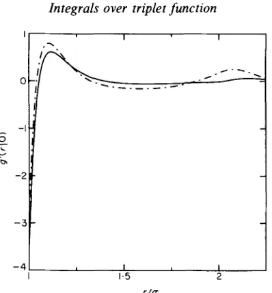
from (16) and (17) for the LJ field of (36). The results for reduced densities po "3 = 0.4 and 0.8 are shown in figures 1 and 2, respectively. At the lower density, g~A(rl0) from (35) largely coincides with the curve in figure 1 and is not plotted. Differences between the two results become more apparent at reduced density 0.8, seen in figure 2. Nevertheless, the two curves are still in relatively good agreement overall.

The calculation then yields by simple quadrature, (30), the second central m o m e n t c2 = m2 - m 2 for the LJ local field carried by hard spheres, tabulated in the table for reduced densities 0.2, 0-4, and 0-8. We list also in this table the first m o m e n t m~ from (27), which of course depends only on the hard sphere

g(r).

These results yield Gaussian shapes that are in good agreement with the local field distributions P(~U) for this model obtained by Monte Carlo simulation by Simon, Dobrasavljevir, and Stratt [ 18]. Unfortunately, no conclusions a b o u t the relative merits of the two calcula- tions for c2 can be drawn f r o m this qualitative comparison.

..,-

-2

- - 5

- 4 I , I

I - 5 2

r/o"

Figure 2.

particle in a hard sphere fluid at density pO "3 = 0"8: ( superposition approximation.

The pair function g'(rl0 ) of (9) for a Lennard-Jones ~k(r) at a hard sphere test ) integral equation; ( . . . )

3.2. The Coulomb field

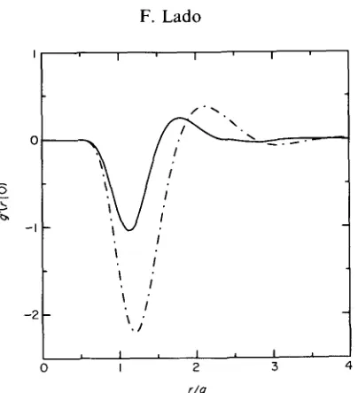
The bridge function and its derivative for the C o u l o m b system were again obtained f r o m the same parametrizations as above [3]. The long-range nature o f the C o u l o m b potential means that some care must be taken in the numerical calculations of its correlation functions. We have followed the prescription o f Ng [23] in dealing analytically with the long range parts o f S ( r l ~ ) and C ( r l ~ ) , leaving only a well behaved short-range residue for the numerical resolution of (16) and (17). Figure 3 displays g ' ( r l 0 ) obtained from the R H N C algorithm o f w and in superposition approximation, (35), at a plasm/~ interaction strength o f F = [3e2/a = 10. We see here a much greater discrepancy between the two calculations c o m p a r e d to the L e n n a r d - Jones/hard sphere results in figures 1 and 2. This disagreement carries over to the c o m p u t e d moments; the curves in figure 3 yield c2 = 0-114 for the integral equation method and c2 = 0.361 using the superposition approximation. There are no simula- tion data for comparison, but internal consistency checks [19] strongly favour the integral equation results, suggesting that the superposition a p p r o x i m a t i o n is not reliable here.

First moment and second central moment of a Lennard-Jones local field at a hard sphere test particle immersed in a hard sphere fluid, from the present integral equation method (IE) and the superposition approximation (SA).

m 2 - -

m~

0.2 - 2.446 0.767 0.754

0-4 - 5.261 1"051 1-017 0.8 -- 11.201 1.072 0-937

po 3 ml SA IE

1394 F. Lado

- c

I I

"~. I .I " .,, --. --,

I I"

-I

' I

i i

'1 _!

-2 "~ /

2 3

rla

4

Figure 3. The pair function g'(r I 0) of (9) for a Coulomb ~b(r) at an ion in a one-component plasma at F = 10: ( ) integral equation; ( . . . ) superposition approximation.

A comment about the Verlet-Weiss parametrization ofgHs(r; a) is appropriate. It has already been noted in other publications [3, 24] that the modelled bridge function obtained from this fit displays a sharp irregularity around r = 2a, leading in turn to a notable spike in a dBHs(r; a)/da in the same region. The numerical effect o f this is likely to be small but used in, say, (18), the result is a decidedly unphysical bump in g'(rl 0) around 2a. This irregularity was part of the motivation for the 'crossover' closure o f Foiles, Ashcroft, and Reatto [24]. Here we have taken the simple expedient of numerically smoothing out the irregularity in the fitted series function SHs(r), which eliminates most o f the anomalous effect, but o f course does not allow for adaption to the known variation with changing potential [25] in the weak, longer-ranged part o f B(r).

We remark further that other parametrizations [26, 27] o f the hard sphere correla- tion functions, while yielding excellent fits to BHs(r; a), also show, for different reasons, similar irregularities in its derivative with respect to a. This is much less true for the analytic solution of Waisman [28], but because o f the highly non-linear equations for its parameters it is harder to use.

I am grateful to Professor Richard M. Stratt for making available the tabulated simulation data used to check the computed moments given in the table.

References

[1] FEENBERG, E., 1969, Theory of Quantum Fluids (Academic Press). [2] McQUARRrE, D. A., 1973, Statistical Mechanics (Harper & Row).

[3] LADO, F., FO1LES, S. M., and ASHCROFT, N. W., 1983, Phys. Rev. A, 28, 2374.

[4] TALBOT, J., LEBOWITZ, J. L., WAISMAN, E. M., LEV~QUE, D., and WEIS, J. J:, 1986, J. chem. Phys., 85, 2187.

[5] MARTYNOV, G. A., and SARKISOV, G. N., 1983, Molec. Phys., 49, 1495. [6] ROGERS, F. J., and YOUNG, D. A., 1984, Phys. Rev. A, 30, 999. [7] ZERAH, G., and HANSEN, J. P., 1986, J. chem. Phys., 84, 2336.

[8] HANSEN, J. P., and McDONALD, I. R., 1986, Theory of Simple Liquids (Academic Press).

[9] LADO, F., 1973, Phys. Rev. A, 8, 2548.

[10] ROSENFELD, Y., and ASHCROFT, N. W., 1979, Phys. Rev. A, 20, 1208. [11] LADO, F., 1982, Phys. Lett., 89A, 196.

[12] FORSTER, D., MARTIN, P. C., and YIP, S., 1968, Phys. Rev., 170, 155. [13] BANSAL, R., and PATHAK, K. N., 1974, Phys. Rev. A, 9, 2773. [14] FELDERHOF, B. U., 1982, J. Phys. C, 15, 3953.

[15] TORQUATO, S., and STELE, G., 1983, J. chem. Phys., 78, 3262. [16] TORQUATO, S., 1991, Appl. Mech. Rev. (to be published). [17] SCHOFIELD, P., 1966, Proc. Phys. Soc., 88, 149.

[18] SIMON, S. H., DOBROSAVLJEVIC, V., and STRATI", R. M., 1990, J. chem. Phys., 93, 2640. [19] LADO, F., 1990, Phys. Rev. A, 42, 7281.

[20] LADO, F., 1987, Phys. Rev. A, 36, 313.

[21] VERLET, L., and WEIS, J. J., 1972, Phys. Rev. A, 5, 939.

[22] HENDERSON, D., and GRUNDKE, E. W., 1975, J. chem. Phys., 63, 601. [23] NG, K. C., 1974, J. chem. Phys., 61, 2680.

[24] FOILES, S. M., ASHCROFT, N. W., and REATTO, L., 1984, J. chem. Phys., 80, 4441. [25] POLL, P. D., and ASHCROFT, N. W., 1987, in Strongly Coupled Plasma Physics, (NA TO A SI

Series, Series B: Physics) edited by deWitt, H. E., and Rogers, F. J. (Plenum).

[26] MALIJEVSKY, A., and LABIK, S., 1987, Molec. Phys., 60, 663; LABIK, S., and MALIJEVSKY, A., 1989, Molec. Phys., 67, 431.

[27] GROOT, R. D., VAN DER EERDEN, J. P., and FABER, N. M., 1987, J. chem. Phys., 87, 2263. [28] WAISMAN, E., 1973, Molec. Phys., 25, 45.