Inference on the Genetic Basis of Eye and Skin Color in an Admixed Population via Bayesian Linear Mixed Models

(1)

| INVESTIGATION

Inference on the Genetic Basis of Eye and Skin Color in

an Admixed Population via Bayesian Linear

Mixed Models

Luke R. Lloyd-Jones,*,1_{Matthew R. Robinson,* Gerhard Moser,}†_{Jian Zeng,* Sandra Beleza,}‡

Gregory S. Barsh,§,††_{Hua Tang,** and Peter M. Visscher*},†† *Institute for Molecular Bioscience and††Queensland Brain Institute, University of Queensland, St. Lucia, Brisbane, Queensland 4072, Australia,†Central Queensland University, Bellbowrie, Brisbane, Queensland 4070, Australia,‡Department of Genetics, University of Leicester, LE1 7RH, United Kingdom,§HudsonAlpha Institute for Biotechnology, Huntsville, Alabama 35806, and **Department of Genetics, Stanford University School of Medicine, Stanford, California 94305

ABSTRACTGenetic association studies in admixed populations are underrepresented in the genomics literature, with a key concern for researchers being the adequate control of spurious associations due to population structure. Linear mixed models (LMMs) are well suited for genome-wide association studies (GWAS) because they account for both population stratiﬁcation and cryptic relatedness and achieve increased statistical power by jointly modeling all genotyped markers. Additionally, Bayesian LMMs allow for moreﬂexible assumptions about the underlying distribution of genetic effects, and can concurrently estimate the proportion of phenotypic variance explained by genetic markers. Using three recently published Bayesian LMMs, Bayes R, BSLMM, and BOLT-LMM, we investigate an existing data set on eye (n= 625) and skin (n= 684) color from Cape Verde, an island nation off West Africa that is home to individuals with a broad range of phenotypic values for eye and skin color due to the mix of West African and European ancestry. We use simulations to demonstrate the utility of Bayesian LMMs for mapping loci and studying the genetic architecture of quantitative traits in admixed populations. The Bayesian LMMs provide evidence for two new pigmentation loci: one for eye color (AHRR) and one for skin color (DDB1).

KEYWORDSadmixed populations; genome-wide association studies; Bayesian linear mixed models; eye and skin color

V

ariation in eye and skin color may be particularly ap-parent in admixed populations, especially those formed from ancestral populations with large differences in these phenotypes. Pigmentation is a diverse phenotype in humans, with most of the variation attributable to differences in the amount, type, and distribution of melanin: a broad term for a set of biopolymers synthesized by melanocytes (Jablonski and Chaplin 2000; Parra 2007). The genetic basis for human pigmentation diversity is yet to be fully understood, but evidence suggests that natural selection shaped the modern

distribution of human pigmentation to be a balance between favoring dark skin near the equator to protect from folate deﬁciency and sunburn, and lighter skin at higher latitudes to allow for optimal vitamin D synthesis (Parra 2007). Genome-wide association studies (GWAS) provide an avenue to further understand the genetic mechanisms underlying this variation. However, GWAS have been predominantly performed in Euro-pean populations, with other ancestral groups and admixed populations underrepresented (Need and Goldstein 2009; Bustamanteet al.2011). Aside from data availability, one key concern for GWAS in admixed populations is the control of spurious associations due to population structure. The large GWAS data sets currently being generated by the genomics community are likely to span multiple ancestral groups, and thus methods that can control for spurious associations in such data sets are of great interest.

There are many methods for correcting for population struc-ture when performing GWAS, with genomic control (Devlin and Roeder 1999), regression control (Wang et al. 2005;

Manuscript received July 4, 2016; accepted for publication March 28, 2017; published Early Online April 3, 2017.

Supplemental material is available online atwww.genetics.org/lookup/suppl/doi:10. 1534/genetics.116.193383/-/DC1.

(2)

Setakiset al.2006), and principal component (PC) adjust-ment (Zhanget al.2003; Priceet al.2006) being the most common approaches. These methods perform well for pop-ulations with simple population structure but may perform poorly when the relatedness structure is more complex or in the presence of cryptic relatedness (Zhao et al.2007). Linear mixed models (LMMs) have been shown to be effec-tive at controlling for population structure and cryptic re-latedness in GWAS; however, they often only consider individual single nucleotide polymorphisms (SNPs) in iso-lation (Gianola et al. 2009; Vilhjálmsson and Nordborg 2013; Yanget al.2014; Lohet al.2015b). LMMs that jointly model marker effects may further increase power in struc-tured populations by capturing the effect of the causal var-iant using multiple markers. Seguraet al.(2012) proposed a multi-locus LMM approach that uses a stepwise selection algorithm to jointly capture weak effects, while Rakitsch

et al. (2013) combined the Lasso (Tibshirani 1996) with the LMM to provide an efﬁcient multi-locus method. Both methods observed higher power and a lower false discovery rate (FDR) than single-locus approaches for mapping. Ex-tensions of the standard LMM, which assumes a single nor-mal distribution on genetic effects, have been made from a Bayesian perspective to include alternative distributions on the genetic effects, and have been applied extensively in the plant and animal breeding literature (Meuwissen et al.

2001; Habier et al. 2011; Erbe et al. 2012; Zhou et al.

2013). Bayesian LMMs (BLMMs) are capable of modeling all markers jointly and have been shown to perform better in prediction than the standard LMM when the genetic archi-tecture of a trait deviates from the inﬁnitesimal model (Goddardet al.2010; Moseret al.2015). Recent implemen-tations of BLMMs are capable of performing genome-wide analyses on a large number of individuals (Zhouet al.2013; Moseret al.2015).

We demonstrate the utility of BLMMs for gene discovery by applying them to eye and skin color phenotypes for individuals from Cape Verde, an island nation off West Africa that is home to individuals with large variation in eye and skin color due to the mix of West African and European ancestry. Beleza

et al.(2013) performed GWAS on the Cape Verde data set, using principal component adjustment to correct for popula-tion structure (using theﬁrst three PCs). In addition, Beleza

et al. (2013) carried out conditional analyses for the most signiﬁcantly associated SNPs, linear regression adjusting for African ancestry and island of birth, and a mixed effect model implemented in the EMMAX software (Kanget al.2010). All three methods used in Beleza et al. (2013) pointed to the same set of genetic loci found in the original PC-adjusted association analysis.

In this work, we apply three recently published BLMM methods – Bayes R (Erbeet al. 2012; Moser et al. 2015), Bayesian sparse LMM (BSLMM) (Zhou et al. 2013), and BOLT-LMM (Loh et al.2015b)–to the unique Cape Verde data set. All three methods can perform gene discovery, var-iance component estimation, and prediction simultaneously,

and assume different priors on the marker effects. This allows for a variation of the assumptions of the inﬁnitesimal model, which is unlikely to hold for the eye and skin color pheno-types present. We explore the potential of BLMM approaches to yield improved power to detect associations in GWAS, particularly in cases where there is substantial confounding due to population structure or cryptic relatedness. Using real genotypes from the Cape Verde data set, we simulate both moderate and highly heritable phenotypes with genetic architectures that contain both small and large effects to demonstrate how BLMM methods can be adapted to iden-tify new quantitative trait loci (QTL) from GWAS. We apply these methods to the Cape Verde data set and identify two additional loci that likely contribute to variation in eye and skin color.

Materials and Methods

Methods overview

The BLMM methods used in this study possess different implementations of a similar underlying model, i.e., the LMM with a ﬁnite mixture of normal distributions used to model the underlying distribution of marker effects. Bayes R (Erbeet al. 2012; Moseret al.2015) and BSLMM (Zhou

et al.2013) estimate the effects of all markers jointly as ran-dom effects, and use Markov chain Monte Carlo (MCMC) to obtain approximate samples from their posterior distribution given the observed data. Methods that use multiple markers to jointly capture the causal QTL effect often lead to higher power and a lower FDR than single marker approaches (Segura et al. 2012; Rakitsch et al. 2013; Moser et al.

2015). Alternatively, BOLT-LMM (Loh et al. 2015b) uses a mixture of two Gaussian distributions to model the marker effects and uses a fast variational approximation to compute approximate phenotypic residuals, with each single marker then evaluated for association with the residuals via a retro-spective score statistic. This method is more powerful than standard single marker regression (as are other similar LMM methods) and provides a bridge between Bayesian modeling and the frequentist association testing framework (Lohet al.

(3)

confounding. We validate these methodological concepts through simulation and via application to the Cape Verde data set.

Cape Verde data set

The Cape Verde data set (Beleza et al. 2013) consists of 625 individuals with high-quality digital eye photographs and 684 individuals with skin reflectance measurements and genotypes. For eye color, Belezaet al.(2013) developed a new measure based on automated analysis of digital pho-tographs that captures the full range of African-European eye color variation. For skin color, reflectance spectroscopy was used on the upper inner arm to calculate a modified melanin index. Genotype quality control was performed as per Beleza

et al.(2013), but with a minor allele frequency (MAF) thresh-old of 0.02 resulting in 858,510 autosomal SNPs. Phenotypes were centered and scaled (by their SD) before regressing the phenotypes on sex and taking the residuals as the new phe-notype. The distribution of the eye and skin phenotypes (standardized to mean 0 and variance 1) showed deviation from normality (Supplemental Material, Figure S1 in File S1). Thus, the continuous phenotypes for eye and skin color were transformed using a rank-based inverse normal trans-formation (Blom 1958).

To explore the level of admixture in the Cape Verde data set, we visualized theﬁrst two projected PCs [implemented in the software of Chenet al.(2016)] relative to the HapMap 3 (International HapMap 3 Consortiumet al.2010) European and African ancestry cohorts (Figure S2 inFile S1). Further-more, to investigate the relatedness of individuals in these data we summarized the diagonals and off diagonals of the genetic relationship matrix, which was estimated using genome-wide marker data in the GCTA software (Yanget al.

2011). For comparison, we also estimated the genetic rela-tionship matrix of a random subset of 685 individuals from a homogeneous European population from the Atherosclerosis Risk in Communities (ARIC) Study (dbGaP accession number phs000090.v1.p1). A summary of the diagonals and off diag-onals of the genetic relationship matrix for both populations shows much greater variance in the Cape Verde population than the European population (Figure S3 and Table S1 inFile S1). The maximum value of the genetic relationship matrix off diagonals of the Cape Verde population is0.25 suggest-ing that the population is not made up of solely unrelated individuals (Figure S3 inFile S1).

Model statement

For each of the methods, the following linear model is used to relate phenotypesyto genotypesX

y¼1nmþXbþe; (1)

whereyis a vector of phenotype values fromnindividuals,X is ann3mmatrix of genotypes measured for each individu-al,bis a vector ofmgenetic effects to be estimated,1nis a

vector of sizenof ones,mrepresents the common phenotypic

mean, andeis a vector of sizenfrom distributionMVNð0;s2 eIÞ;

where Iis the identity matrix. The elements of Xare 0, 1, 2 encoded genotypes and represent the counts of the refer-ence allele at each ofmmarkers. Whether the columns ofX are centered and/or standardized depends on the method used, with Bayes R mean standardized and scaled to have variance 1, BSLMM mean centered only, and BOLT-LMM mean centered and standardized to have common variance (Loh et al. 2015b). Standardizing the columns of X corre-sponds to making an assumption that rarer variants have larger effects than common variants (Zhouet al.2013). To provide a baseline for comparison with the results generated by the BLMMs, associations between each SNP and the phe-notypes (adjusted for sex) were assessed using the marginal regression model (i.e., standard GWAS). Similar to Beleza

et al. (2013), thefirst 10 PCs were fitted as covariates to adjust for population stratification with the analyses per-formed using the PLINK 2 software (Changet al.2015).

Bayesian linear mixed models

Bayes R:Erbeet al.(2012) were theﬁrst to present the Bayes R method, which uses a Bayesian hierarchical linear random regression model and poses the following four component mixture priors for each SNP effect in model (1):

bj p1N 0;03s2g

þp2N 0;10243s2g

þp3N 0;10233s2g

þp4N 0;10223s2g

; (2)

where j2 ð1;. . .;mÞ is an index over the SNPs, s2 g is the

additive genetic variance explained by SNPs, and p1 is the proportion of SNPs that have no effect. In practice, the true distribution of genetic effects is not known and thus one of the strengths of this prior is its ﬂexibility to approximate various underlying distributions. Depending on prior knowl-edge or cross-validation, the model can accommodate fewer or.4 components and larger variance classes (i.e., changing the multiplier of s2

g for any of the mixture components

1022_/₁₀21_{for instance). The model}_{fits all SNPs} simulta-neously, which accounts for linkage disequilibrium (LD) be-tween SNPs, and increases power to detect associations (as do other methods) (Erbeet al.2012; Moseret al.2015). The model also induces sparsity via the first component of the mixture, thusfitting with the hypothesis that not all markers are in LD with a causal variant. Moseret al.(2015) incorpo-rated a hyper-parameter for the variance explained by ge-nome-wide SNPs, s2g; which allows for the proportion of

phenotypic variance explained by genotyped SNPs (PVE) to be estimated from the data, rather thanﬁxing it prior to anal-ysis as in Erbeet al.(2012).

BSLMM: BSLMM (Zhou et al. 2013) summarizes the two ends of the spectrum with respect to the assumption of the distribution of genetic effects, where the LMM assumes every variant has an effect, and the sparse BLMM assumes that a very small proportion of variants have an effect. Zhouet al.

(4)

would vary depending on the true underlying genetic archi-tecture of the phenotype. BSLMM is a hybrid approach that includes the LMM and sparse regression model as special cases and is capable of learning the genetic architecture from the data. Additionally, BSLMM makes estimation of this type tractable for reasonably large data sets using linear algebra tricks for LMMs. Bayes R and BSLMM report the posterior probability that a polymorphic site affects the trait condi-tional on the data, which is a very natural statistic to interpret in the context of QTL identiﬁcation. For these methods, the posterior inclusion probability (PIP) summarizes the number of times a locus was present in the model.

Zhouet al.(2013) assume thatbjfrom Equation (1) comes

from a mixture of two normal distributions:

bj pN 0; s2aþs2b

ðmtÞþ ð12pÞN 0;s2_bðmtÞ;

where setting p¼0 yields the LMM, and setting sb¼0

yields the sparse regression model in which a subset of SNPs is assumed to have no effect (noninﬁnitesimal model),mis the number of genetic markers, andtis the reciprocal of the residual variance. This model can be interpreted as all vari-ants have at least a small effect, which are normally distrib-uted with variance s2

b=ðmtÞ; and some proportion p of

variants that have an additional effect that is normally dis-tributed with variances2

a=ðmtÞ:

BOLT-LMM: BOLT-LMM (Loh et al.2015b) relaxes the as-sumptions of the inﬁnitesimal model by using a mixture of two Gaussian distributions as the prior onbjin Equation (1),

giving the model greaterﬂexibility to accommodate SNPs of large effect while maintaining effective modeling of genome-wide effects (for example, ancestry). The noninﬁnitesimal component amounts to a generalization of the standard mixed model, which places a spike-and-slab mixture of two Gaussian priors on SNP effect sizesi.e.,

bj pN 0;s21

þ ð12pÞN 0;s2₂;

wherepis the mixing proportion ands2

1ands22the variances of the two Gaussians. This assumption gives the model greaterflexibility to accommodate SNPs of large effect while modeling genome-wide effects. Lohet al.(2015b) note that it is important that the spike component have nonzero variance to capture genome-wide ancestry or relatedness effects. When testing SNPs for association, effects attributed to the random component, for all other chromosomes except that of the SNP being tested [also referred to as a leave one chromo-some out (LOCO) approach (Yang et al.2014)], are condi-tioned out from the phenotype and the final association is performed on the residuals of this conditioning step, which protects against confounding (Loh et al. 2015b). BOLT-LMM uses a variational approximation tofit Bayesian linear regressions for the Gaussian mixture priors rather than MCMC as in Bayes R and BSLMM. BOLT-LMM uses cross-validation to estimate hyper-parameters for the variational

algorithm, rather than relying on variational approximate log-likelihoods, because it was found to be more robust to slackness of the variational approximation caused by LD (the variational approximation is a good approximation when the SNPs X are independent; Carbonetto and Stephens 2012). BOLT-LMM could also be viewed as a hybrid methodology that applies a retrospective hypothesis test for association of the left-out SNPs with the residual phenotype. This is a key point of difference from Bayes R and BSLMM which report a PIP for each SNP, whereas BOLT-LMM retains the classical hypothesis test approach. Lohet al.(2015b) simulated phe-notypes that included an ancestry effect and found that the BOLT-LMM chi-squared statistics were well calibrated in terms oflGCand the mixed-model analysis achieved

statisti-cally significant gains in power over principal component analysis (PCA) across simulations. The genomic inflation fac-torlGCis defined as the ratio of the median of the empirically

observed distribution of the association test statistic to the expected median (from the x2

1 distribution) (Devlin and Roeder 1999).

Implementation of BLMM methodology

For Bayes R [implemented in the software provided in Moser

et al.(2015)], we assumed the prior in Equation (2) with a 5% largest class. Additional prior assumptions were made as per the default of the program provided in Moser et al.

(2015). The 5% variance class was used because previous estimates of variance explained for large-effect loci from eye and skin color were of this order, as reported in Beleza

et al.(2013). To monitor convergence of the MCMC chains, we ran two chains with 100,000 iterations and 20,000 burn iterations and another for 200,000 iterations with 40,000 burn in iterations, which included permuting the SNP order to improve mixing, and a thinning rate of 1 in every 10 iter-ations. We compared the results from the two chains, and investigated the agreement between the estimates of the PVE and the rank of the top regions for both eye and skin color. For BSLMM, we similarly ran a short and long chain, one with 1 million iterations with 100,000 burn in (program default) and a longer chain of 2 million iterations with 100,000 burn in. When implementing the BOLT-LMM soft-ware, an LD score table is required. The LD score table was generated for the Cape Verde data set using the available software (Bulik-Sullivanet al. 2015). This table was subse-quently used when running the BOLT-LMM program.

Association inference from BLMMs

(5)

rather than on individual markers. To construct a posterior distribution for the proportion of genetic variance explained by markers in a genomic region we divide the genome into 1-Mb nonoverlapping regions. For each iteration t of the MCMC chain we calculate for each windoww2 ð1;. . .;WÞ

the genetic variances2gððwtÞÞ ¼VarðXwbtwÞ;whereXwis the

ma-trix of SNPs in the window andbtwthe estimated effects for

the SNPs in the window. Additionally, for each iteration we calculate the total genetic variance ass2gðtÞ¼VarðXbtÞ:The

ratio between the window variance and total genetic vari-ance for each iterationt:

rt_w¼s

2ðtÞ

gðwÞ

s2ðtÞ

g

deﬁnes the proportion of the total genetic variance explained by the window. We form the posterior distribution forrt

w by

calculating this value for each of titerations in the MCMC chain. We compute the posterior probability that a windoww

explains .1% (for example) of the total genetic variation by calculating the ratio of the number of iterations that

rt

w.0:01 divided by the total number of MCMC iterations T, which is deﬁned to be the window posterior probability of

association [WPPA; Fernando and Garrick (2013)]. It can be shown that using a threshold of WPPA¼ato conclude that a locus is associated with the phenotype will result in control-ling the proportion of false positives (PFP) to be ,12a (Fernando and Garrick 2013; Zeng 2015). The posterior probabilities contributing to these calculations require that the priors placed on the unknown variables in the model are identical to those used to generate these variables (Fernando and Garrick 2013). Unfortunately, this is unlikely to be the case, but as data size increases the posterior distributions will become increasingly independent of the priors used. Control-ling the PFP has the added beneﬁts of it being independent of the number of tests performed and does not require indepen-dence of tests (Fernandoet al.2004). Bayes R allows for the nonzero SNP effects for each iteration to be saved to ﬁle, which facilitates these calculations post analysis.

BSLMM does not report the genetic effect from each MCMC iteration and thus we cannot implement a similar method of inference to that of Bayes R. However, Guan and Stephens (2011) suggest calculating the posterior expected number of SNPs in a window by summing the estimated PIPs for all genetic variants in that region (denoted WPIP). We use this measure to summarize the results from BSLMM at the levels of regions and compare with the inference from the WPPA.

Loci associated with ancestry

To examine the degree of allelic differentiation across the ancestral gradient of SNPs in the Cape Verde data set, we used the method presented in Galinskyet al.(2016), which gen-eralizes a previous method for detecting allele frequency differences between subpopulations to populations with fractional ancestry. The method uses the SNP weights from PCA to calculate a statistic that measures the differentiation

of each SNP along the ancestral gradient. Galinsky et al.

(2016) outline that the statistic is calculated as the dot product Dj¼yjvk; wherevk is the kth eigenvector of the normalized genotype matrix and y_j is the jth normalized SNP. As per Galinskyet al. (2016), the set ofD2 statistics for all of p SNPs has a x2

1 distribution after appropriate rescaling, which allows for hypothesis testing for each SNP to be performed. Inference can then be made about which loci are highly differentiated along the ancestral gra-dient. It is proposed that if the top associations for eye and skin color do not lie in the set of lowestP-values after mul-tiple testing correction, then this is further evidence that the set of loci detected is less likely to be spurious due to struc-ture. Additionally, we use the set of statistics to rank the set of genotype SNPs for use in simulating phenotypes that are correlated with ancestry. For highly associated SNPs (eye and skin color) we only report D2 statisticP-values for PC one as it captures most of the ancestral differences (Figure S2 inFile S1). Estimation of theﬁrst 10 PCs of the genotype matrix was performed using theﬂashpca software (Abraham and Inouye 2014).

Simulation study

The Cape Verde data provide an opportunity to understand the performance of the BLMM methods relative to standard methods in an admixed sample. Speciﬁcally, we wanted to assess how BLMMs perform in terms of gene discovery and PVE estimation, under simulated genetic architectures that are similar to those hypothesized for eye and skin color. We used the simulations to infer the PIP that allows for conﬁdence in making statements about whether a 1-Mb window around the causal variant is associated with the trait conditional on the data. Each of the simulation scenarios used the real ge-notype data (n= 685) from Cape Verde.

(6)

Additionally, a single SNP association analysis (analyzed in PLINK 2) corrected for 10 PCs was run for gene discovery comparison and a PVE estimation benchmark was carried out using the widely used GREML approach (Yang et al.

2010) in the GCTA software (Yanget al.2011).

Scenario two retained the same proportions of phenotypic variance for the randomly sampled 5 and 45 causal loci (and PVE of 0.9) but placed genetic effects on loci that were differentiated across the admixture gradient (as outlined in the sectionLoci associated with ancestry). It was hypothesized [and supported by results in Beleza et al.(2013)] that eye and skin color are correlated with ancestry; therefore, in or-der to simulate these traits more realistically we generated 50 phenotypes by randomly selecting 50 loci that were asso-ciated with theﬁrst PC (implicitly assuming that PC one is a good proxy for ancestry as demonstrated in Figure S2 inFile S1). To generate the list of SNPs, we took the list of D2 statistics and subsetted it to those loci that had P-values

,131022 _but _.₁₃₁₀23 ₍_11;₀₀₀_{SNPs). This list} in-cludes SNPS that were differentiated across the ancestral gradient but were not the“most”differentiated. This decision was made by investigating theD2statisticP-values for the top loci found in Belezaet al.(2013), which showed that most of the top loci were differentiated but with P-values .1023_: This list was furtherfiltered by LD to independent loci using the PLINK clumping procedure. Thefinal list of SNPs con-sisted of 3500 PC-one-associated SNPs. Again Bayes R (5% largest variance class), BSLMM, and BOLT-LMM were run for each realization with a single SNP association anal-ysis (run in PLINK) corrected for 10 PCs and PVE estima-tion in the GCTA software completed for comparison. Simulation Scenarios Three and Four were a repeat of the first two but with the 45 small-effect loci explaining 30% of the phenotypic variance, the five large-effect loci 20%, and a PVE value of 0.5. For both of these simulations Bayes R was run with a 1% largest variance class as the causal loci explained less variance.

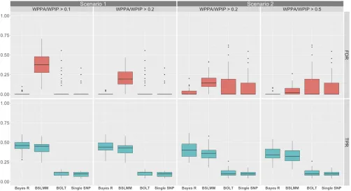
Methods were assessed across simulation scenarios for their ability to identify genomic regions containing simulated causal SNPs. Two performance measures were used to sum-marize the results namely: the true positive rate (TPR) for detecting a 1-Mb window containing a simulated causal variant and the FDR for detecting a 1-Mb window containing a simulated causal variant. For the BOLT-LMM and PLINK association analyses, a 1-Mb window was deemed to be a true positive if it contained an SNP that passed genome-wide signiﬁcance and was a member of the simulated windows that contained a causal SNP. For Bayes R and BSLMM, a 1-Mb window was deemed to be a true positive if it had a WPPA (of explaining .1% of the genetic variance) or WPIP greater than a thresholdaand was one of the simulated windows that contained a causal SNP. For each method, the TPR was calculated as the number of true positive regions/number of simulated regions containing a causal SNP. The FDR was calculated as the (number of regions that passed the threshold 2number of true positives)/number of regions

that passed the threshold. These measures were summa-rized for each scenario for all methods with different a thresholds on WPPA and WPIP for Bayes R and BSLMM explored.

Furthermore, we investigated the control of the PFP for varying thresholds on the Bayes R WPPA. To achieve this, for each a threshold on the WPPA in the set

ð0:05;0:1;0:2;0:3;0:4;0:5;0:6;0:7;0:8;0:9;0:95Þwe calcu-lated the observed PFP across the 50 replicates for each simulation scenario. A region was declared a false positive if it passed the aWPPA threshold but did not contain a simulated causal variant.

Simulation two: In the second simulation we focused on investigating the PVE for large-effect loci and again summa-rized the ability of each method to estimate total PVE with an altered genetic architecture. This simulation investigated the hypothesis that confounding contributes less to loci that explain a substantial amount of the genetic variance. The sum of the contribution of only highly associated regions is but a portion of the total genetic variance because it ignores the contribution from loci that may explain genetic variance but do not show strong evidence for association. Therefore, it is hypothesized that the sum of the estimated PVE for highly associated regions should be a reasonable lower bound to the total PVE for a trait and should be relatively free of confounding. We test this hypothesis with simulation in order to guide the conclusions made about the contribution to PVE for the top loci detected for eye and skin color in the Cape Verde population.

(7)

Data availability

Tables S7–S12 contain detailed results on detected loci for eye and skin color for the Bayes R, BSLMM, and BOLT-LMM methods and can be found inFile S2. The following freely available programs were used to complete the analyses: BayesR (www.github.com/syntheke/bayesR), BOLT-LMM (www.hsph.harvard.edu/po-ru-loh/software/), GCTA (www. cnsgenomics.com/software/gcta/), GEMMA (http://www. xzlab.org/software.html), and PLINK (www.cog-genomics. org/plink2).

Results

Simulation study

Simulation one: Bayes R and BSLMM performed substan-tially better (higher TPRs) than BOLT-LMM and single SNP analysis for more highly heritable traits and in the absence of confounding due to stratiﬁcation (scenarios one and three, Figure 1 and Figure S4 inFile S1), but persisted even in the presence of confounding (scenarios two and four, Figure 1 and Figure S4 inFile S1). Thresholding on the WPPA con-trolled the proportion of false positives to be ,(12a) but appeared to be too stringent with a WPPA threshold of 0.5 leading to a PFP between 0.05 and 0.1 across simulation scenarios (Figure S5 inFile S1). For each of the simulation scenarios anathreshold of 0.95 resulted in an approximate PFP of 1% and at 0.92%. These results suggest that a WPPA and WPIP threshold of 0.5 is reasonable for concluding that a region has evidence that it is associated with the eye and skin color traits in these data. This conclusion rests on the assump-tion that pigmentaassump-tion traits are moderately heritable and are driven by loci that are in part differentiated along the ances-tral gradient in the Cape Verde population.

For estimates of PVE (Figure S6 inFile S1), two general trends emerged. In the absence of confounding due to strati-fication (scenarios one and three), all four methods exhibited upward bias with regard to PVE estimation (more apparent in scenario three). However, in the presence of confounding due to stratification (scenarios two and four), all four methods overestimated PVE, consistent with what was originally de-scribed for BOLT-LMM (Lohet al.2015a). Second, PVE es-timates from BOLT-LMM and GCTA showed much more variance than that of Bayes R or BSLMM. Taken together, the results of simulation one suggest that applications of BLMM approaches in the Cape Verde population are most useful for gene discovery and identification of causal vari-ants, as we describe below.

Simulation two:Simulation two again suggests that BLMM/ LMMs exhibit an upward bias (when simulated with geno-types from Cape Verde) with regard to PVE estimation espe-cially in the presence of confounding due to stratiﬁcation (Figure S7 inFile S1). Potential reasons for the upward bias from the BLMMs across simulations are the inclusion of many small effects, as there exists a nonzero probability that any

one SNP can be included in the model, and thus given the small sample size, the Bayesian methods include many small effects that cannot be set to 0 with certainty. This is likely to reflect overfitting given the large number of parameters rel-ative to the sample size. This upward bias is hypothesized to be exacerbated when the effects are aligned with ancestry, as observed, due to markers capturing the population stratifica-tion. However, for these scenarios no individual noncausal SNP had a high inclusion probability or large effect across all iterations (i.e., posterior mean), and thus in each iteration there is a different set of null effects that sum to a nonzero heritability. These conclusions also apply to results from sim-ulation one. For thefive causal loci of large effect, the BLMMs have a small downward bias in the PVE when compared to estimates from PLINK (Figure S8 inFile S1). However, the simulation shows that summing the proportion of phenotypic variance for regions surrounding the causal variant achieves a reasonable lower bound for the true PVE for large-effect loci and thus for the total PVE.

Loci associated with eye and skin color

For Bayes R, the rank of the top loci and WPPA, distributions of the genetic variance for the top regions, the posterior means of the PVE, and the number of loci in the largest variance class all remained stable for both eye and skin color when the results from the longer chain were compared with the shorter chain (Figures S9–S12 and Tables S2 and S3 in File S1). For BSLMM, we saw a similar stability in the rank and WPIP of the top loci for eye and skin color and the posterior mean of the PVE between the long and short chains (Figures S13 and S14 and Tables S4 and S5 inFile S1). We therefore treat the results from the longer chains as a representative sample from the target distribution for each of the parameters of interest. Results from the Bayes R model are based on the longer chain run (200,000 iterations with 40,000 burn in), which includes 16,000 iterations after thinning (1 in 10). Similarly for BSLMM, posterior estimates were generated from the longer chain of 2 M iterations with 200,000 ele-ments from the longer chain after thinning.

(8)

rs12913832 and rs1426654 SNPs (HERC2 and SLC24A5) (Table 1). The rs1426654 SNP has an LDR2 _{of 0.99 with} the rs2470102 SNP reported as the top association in Beleza

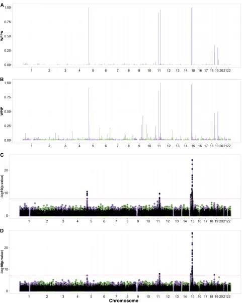
et al. (2013). Within the chromosome 5 locus, the rs7736 SNP showed smaller PIPs of 0.06 and 0.05 for the top SNP (Table 1). The results from Bayes R and BSLMM show that there are many variants contributing to the regional associ-ation signal on chromosome 5 with smaller PIPs spread across many SNPs (Figure S15A inFile S1and Table S7 in

File S2). Additionally, Bayes R and BSLMM show high PIPs for the SNP rs1635166 (0.67 and 0.90, respectively) sug-gesting that for the HERC2 locus there may be.1 causal SNP generating associations (Figure S15B inFile S1). The LDR2 _{of the rs1635166 SNP with rs12913832 is relatively} small (0.25), further supporting this hypothesis (Table S6 in

File S1). BOLT-LMM reportedlGCstatistics of 0.99 for the

inﬁnitesimal statistics and 0.99 for the noninﬁnitesimal sta-tistics (Figure S16 in File S1). The standard linear model analysis corrected for 10 PCs reported similar top loci to those of Beleza et al. (2013) (Figure 2D). The standard linear model analysis reported rs7736 (5:731027_{) as the} top SNP at the chromosome 5 locus.

The degree of allelic differentiation across the ancestral gradient, summarized by theD2statistics, for the most highly associated SNPs showedP-values that did not pass genome-wide significance suggesting that these SNPs are not mark-edly differentiated across thefirst PC (Table 1). However, no SNP passed genome-wide significance for the allelic differen-tiation across the ancestral gradient analysis with the top SNP having an associationP-value of 3:631026_:_{This shows that} the associated SNPs for eye color are not the most differen-tiated across the ancestral gradient.

Each of the three BLMM methods showed moderate evi-dence for an association on chromosome 5 not reported in Belezaet al.(2013). The locus zoom plots showed a strong LD pattern extending across a region of several hundred kilobases that includes six genes of which one,AHRR (aryl-hydrocarbon receptor repressor), is a plausible candidate (Figure S15A inFile S1). Originally recognized as a homo-log of the arylhydrocarbon receptor (AhR) gene,AHRR en-codes a bHLH-PAS protein that binds to the same response element as AhR but represses AhR signaling.AHRRis widely expressed, and in zebraﬁsh embryos, morpholinos against anAHRRparalog,AHRRa, elicit changes in gene expression

(9)

(10)

thought to reﬂect a role in eye development and function (Aluruet al.2014).

Skin color: In the original GWAS, Belezaet al.(2013) re-ported four loci for skin color on chromosomes 5, 11, and 15 with candidate genesSLC45A2,GRM5/TYR,APBA2, and

SLC24A5. Bayes R, BSLMM, and BOLT-LMM all reported these regions as showing evidence for association and, in addition, revealed evidence for a new region on chromo-some 11. Bayes R and BSLMM reported WPPA and WPIP values .0.92 for the four loci identiﬁed in Beleza et al.

(2013) with BOLT-LMM reporting SNPs passing the genome-wide signiﬁcance for each of the regions (Figure 3 and Table 1). Among the genes present in the additional region on chromosome 11 recognized by the BLMM methods, the

DDB1gene is a plausible candidate for regulating variation in skin color (Figure S15C inFile S1).DDB1is involved in nucleotide excision repair following UV-induced DNA dam-age, and therefore could play a role in the tanning response and/or photosensitivity (Liuet al.2000; Bekker-Jensenet al.

2010). Bayes R and BSLMM reported strong evidence for this locus with a WPPA = 0.91 and a WPIP = 0.86 that this region is associated with skin color. The SNP with the smallest

P-value from BOLT-LMM (rs2513329) did not reach genome-wide signiﬁcance (P-value = 5:231027_{). The Bayes R and} BSLMM PIPs for the rs2513329 SNP (Table 1) in theDDB1

region were smaller than those for a second SNP located in the same region (rs10792312 PIP = 0.46 and 0.76), which has an LDR2 _{of 1.0 with rs2513329 (Table S6 in}_{File S1}_). Similar to the chromosome 5 locus for eye color, theGRM5/

TYRlocus showed many variants contributing to the regional association with no one variant showing a PIP.0.3 (Tables S10 and S11 inFile S2).

BOLT-LMM only reported the inﬁnitesimal model statistics for skin color with alGCvalue of 1.04 (Figure S16 inFile S1).

The linear association analysis corrected for 10 PCs reported similar top loci to those by Belezaet al.(2013) (Figure 3D). The degree of allelic differentiation across the ancestral

gradient analysis, summarized by theD2 statistics, for the most highly associated SNPs showed allelic differentiation

P-values that did not pass genome-wide, suggesting that these SNPs are not markedly differentiated across theﬁrst PC (Table 1).

Proportion of phenotypic variance explained by highly associated regions:Given the evidence from the three mod-els, three regions for eye color showed the most evidence for association. These were the AHRRgene region on chromo-some 5, and theHERC2/OCA2andSLC24A5gene on chro-mosome 15. The distribution of the genetic variance was generated as a by-product of the WPPA calculation and thus from these analyses we calculated the posterior means for the PVE by dividing the estimated genetic variance for each re-gion for each iterationtby the estimated phenotypic variance s2

gþs2e for each iteration. The three regions for eye color

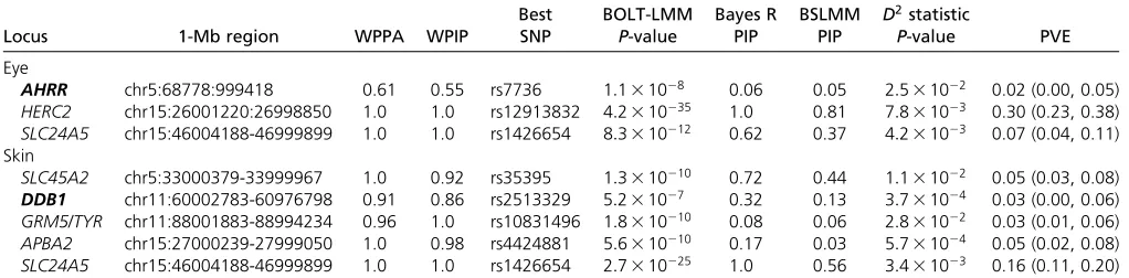
(AHRR,HERC2/OCA2,SLC24A5) explained 2.0% (0.0, 5.0), 30% (23, 38), and 7.0% (4.0, 11) of the phenotypic variance for eye color, respectively (intervals in parentheses indicate the 95% credible interval for these estimates calculated using quantiles). These three regions explained 39% (32, 46) of the phenotypic variance for eye color (Table 1).

For skin color, theﬁve regions with the most evidence for association wereSLC45A2,GRM5/TYR,APBA2, andSLC24A5, and the additional region ofDDB1. These regions explained 5.0% (3.0, 8.0), 3.0% (1.0, 6.0), 5.0% (2.0, 8.0), 16% (11, 20), and 3.0% (0.0, 6.0) of the phenotypic variance, respec-tively (Table 1). The total proportion of genetic variation explained by the topﬁve regions with evidence for association was 32% (26, 38).

Discussion

The use of BLMMs in the heavily admixed Cape Verde pop-ulation has led to evidence for additional associations for eye and skin color when compared to those reported by Beleza

et al.(2013). The results from the BLMMs are consistent with

Table 1 Summary of the top loci from Bayes R, BSLMM, and BOLT-LMM

Locus 1-Mb region WPPA WPIP

Best SNP

BOLT-LMM P-value

Bayes R PIP

BSLMM PIP D

2_statistic

P-value PVE Eye

AHRR chr5:68778:999418 0.61 0.55 rs7736 1:131028 _0.06 _0.05 ₂_:₅₃₁₀22 _{0.02 (0.00, 0.05)} HERC2 chr15:26001220:26998850 1.0 1.0 rs12913832 4:2310235 _1.0 _0.81 ₇_:₈₃₁₀23 _{0.30 (0.23, 0.38)} SLC24A5 chr15:46004188-46999899 1.0 1.0 rs1426654 8:3310212 _0.62 _0.37 ₄_:₂₃₁₀23 _{0.07 (0.04, 0.11)} Skin

SLC45A2 chr5:33000379-33999967 1.0 0.92 rs35395 1:3310210 _0.72 _0.44 ₁_:₁₃₁₀22 _{0.05 (0.03, 0.08)}

DDB1 chr11:60002783-60976798 0.91 0.86 rs2513329 5:231027 _0.32 _0.13 ₃_:₇₃₁₀24 _{0.03 (0.00, 0.06)} GRM5/TYR chr11:88001883-88994234 0.96 1.0 rs10831496 1:8310210 _0.08 _0.06 ₂_:₈₃₁₀22 _{0.03 (0.01, 0.06)} APBA2 chr15:27000239-27999050 1.0 0.98 rs4424881 5:6310210 _0.17 _0.03 ₅_:₇₃₁₀24 _{0.05 (0.02, 0.08)} SLC24A5 chr15:46004188-46999899 1.0 1.0 rs1426654 2:7310225 _1.0 _0.56 ₃_:₄₃₁₀23 _{0.16 (0.11, 0.20)} The WPPA and WPIP are reported for the stated 1-Mb regions with hg18 bp coordinates. For each region the best SNP refers to the SNP in the region with the smallest P-value from BOLT-LMM. For the eye colorHERC2locus the PIP for Bayes R is with reference to the SNP rs1129038, which has an LDR2_{of 0.98 with the rs12913832 SNP. For}

Bayes R the PIP for each SNP is that of being in the model,i.e., the sum of the PIP of being in any of the nonzero variance classes and for BSLMM the PIP corresponds to the SNP having an effect above the polygenic background. Rows containing bold gene names are potentially novel relative to those found by Belezaet al.(2013). TheD2_statistic

(11)

(12)

the top regions presented in Belezaet al.(2013), and avoid the choice of the number of PCs required to control for spu-rious associations (as do frequentist versions of the LMM) due to ancestral differences. The use of concordant evidence across the three BLMM methods, coupled with biological an-notation, indicates a potential involvement of theAHRRgene region for eye color and theDDB1gene region for skin color. The moderate WPPA and WPIP values for the AHRR gene locus were reinforced by a genome-wide signiﬁcant result for the rs7736 SNP from BOLT-LMM. Given the high WPPA and WPIP for the locus in theDDB1 gene, and the central role in DNA repair post UV damage that the protein product of this gene encodes, we argue that this is statistically the most suggestive locus for an effect on skin color not detected by the PC-corrected linear model approach.

The results for eye and skin color are further supported by the simulations where for highly heritable traits, Bayes R and BSLMM retained higher TPRs for the same FDRs than the BOLT-LMM and standard GWAS methods (at a genome-wide significance threshold), which is likely derived from their ability to jointly capture the effect of a causal variant using multiple SNPs simultaneously (Guan and Stephens 2011; Segura et al.2012; Moser et al.2015). This loss in power was seen in the results for the chromosome five locus for eye color, where PC adjustment resulted in associations not being genome-wide significant relative to the BOLT-LMM re-sults. This suggests that for discovery of new associations, BLMMs may be a potential improvement over currently implemented LMM methodology in structured populations. The results from simulation 1, scenarios 1 and 2 show that Bayes R has a higher median TPR and a lower median FDR than BSLMM for a given WPPA and WPIP threshold. This may be driven by the ability of Bayes R to better model the large genetic effects for these simulated traits, which are generated by the high PVE in these scenarios. This is further reinforced by the convergence of the median TPR and FDR for Bayes R and BSLMM in scenarios 3 and 4, which have a simulated PVE = 0.5. This suggests that for more polygenic traits, Bayes R and BSLMM are expected to perform equally well at map-ping loci, a result observed in Moseret al.(2015). As BSLMM does not allow for the calculation of the WPPA statistics, the comparisons made between the median TPR and FDR across simulation scenarios are not optimal. It is difficult to evaluate how much of this difference is due to practical rather than fundamental (such as the prior distribution on the genetic effects) reasons. We also demonstrated that for each of the simulation scenarios that the PFP was controlled to be be-tween 5 and 10% when a WPPA threshold of 0.5 was applied. This lends further evidence to the association results in the

AHRRandDDB1loci, which had a WPPA/WPIP of 0.6/0.55 and 0.91/0.86 respectively.

Previous estimates of PVE indicate that eye and skin color are highly heritable with estimates for both traits ranging between 0.7 and 0.9 (Bräuer and Chopra 1978; Byard 1981). One consequence of the deﬁnition of heritability is that it is a population-speciﬁc parameter, because both the variation in

additive genetic factors (and nonadditive), as well as the environmental variance, are population speciﬁc (Visscher

et al.2008). For traits simulated using the Cape Verde geno-types, the median estimates of PVE from BSLMM/LMMs were upwardly biased and showed large variation, with medians hitting the boundary at unity in some scenarios. These results suggest that PVE estimation using BLMM/LMMs is unreliable for the Cape Verde data set. The LD score regression method (Bulik-Sullivanet al.2015) is a recent development for dis-tinguishing between inﬂated test statistics due to confound-ing bias and polygenicity. This method suggests one avenue for removing confounding from population structure from the heritability estimate but is yet to be extended to admixed populations (Bulik-Sullivanet al.2015). Bayesian LMMs cou-pled with PC correction, or a generalized LD score regression, may be avenues for unbiased PVE estimation, which would require extensive simulations in a much larger data set with empirical data to validate. However, estimates of PVE from regions surrounding purported highly associated loci should provide a reasonable lower bound for the narrow-sense her-itability as seen in simulation two. The results from the PVE for top associated loci are very similar to those reported for skin color in Belezaet al.(2013), which concluded that the four major loci contribute a total of 35% to skin color varia-tion. Our results suggest that the PVE for the topﬁve loci was 32% (26, 38) with the SLC24A5locus contributing16% and theDDB1locus explaining an additional 3%. This high-lights that although BLMMs and marginal linear regression both provide comparable estimates of PVE for an individual locus of large effect, the BLMMs allow for additional loci to be detected.

The posterior probability that a polymorphic site affects the trait conditional on the data is a very natural statistic to interpret in the context of QTL identiﬁcation (Viallefont

(13)

of effects and the sensitivity to prior assumptions are mitigated by using a regional measure of association such as the WPPA, where uncertainty is averaged across the region. Alternatively, Wen (2015) derived Bayes factors for results generated from the LMM methodology, which could also be used as a primary statistical device for model comparison. It is important to point out thatP-values convey a strength of evidence that depends on factors that affect power, which is not a concern for the posterior probability of association statistics provided by the Bayesian methods (Stephens and Balding 2009). We believe that the results of this paper suggest that Bayesian LMM-based methods coupled with a theoretically justiﬁed method for con-trolling the false-positive rate could be a very effective tool for mapping new genetic loci. However, more rigorous frame-works for prior choice and assessment of signiﬁcance and un-certainty in genetic effects from Bayesian LMMs are needed, which is an interesting open question.

Acknowledgments

This work was supported by the Australian National Health and Medical Research Council (1080157 to G.M.) and US National Institutes of Health (NIH) (R01MH100141). ARIC: The Atherosclerosis Risk in Communities Study (dbGaP accession number phs000090.v1.p) is carried out as a collab-orative study supported by National Heart, Lung, and Blood Institute contracts (HHSN268201100005C, HHSN26820-1100006C, HHSN268201100007C, HHSN268201100008C, HHSN268201100009C, HHSN268201100010C, HHSN26820-1100011C, and HHSN268201100012C), R01HL087641, R01HL59367, and R01HL086694; National HumanGenome Research Institute contract U01HG004402; and National Institutes of Health contract HHSN268200625226C. The authors thank the staff and participants of the ARIC study for their important contributions. Infrastructure was partly sup-ported by grant number UL1RR025005, a component of the NIH and NIH Roadmap for Medical Research.

Literature Cited

Abraham, G., and M. Inouye, 2014 Fast principal component

analysis of large-scale genome-wide data. PLoS One 9: e93766.

Aluru, N., M. J. Jenny, and M. E. Hahn, 2014 Knockdown of a

zebraﬁsh aryl hydrocarbon receptor repressor (AHRRa) affects expression of genes related to photoreceptor development and hematopoiesis. Toxicol. Sci. 139: 381–395.

Bekker-Jensen, S., J. R. Danielsen, K. Fugger, I. Gromova, A. Nerstedt

et al., 2010 HERC2 coordinates ubiquitin-dependent assembly of DNA repair factors on damaged chromosomes. Nat. Cell Biol. 12: 80_–86.

Beleza, S., N. A. Johnson, S. I. Candille, D. M. Absher, M. A. Coram

et al., 2013 Genetic architecture of skin and eye color in an African-European admixed population. PLoS Genet. 9: e1003372.

Blom, G., 1958 Statistical estimates and transformed beta-variables. Ph.D. Thesis, Stockholm College, Stockholm, Sweden.

Bräuer, G., and V. P. Chopra, 1978 Estimation of the heritability of hair and eye color. Anthropol. Anz. 36: 109_–120.

Bulik-Sullivan, B. K., P.-R. Loh, H. K. Finucane, S. Ripke, J. Yang

et al., 2015 LD score regression distinguishes confounding from polygenicity in genome-wide association studies. Nat. Genet. 47: 291–295.

Bustamante, C. D., M. Francisco, and E. G. Burchard,

2011 Genomics for the world. Nature 475: 163–165. Byard, P. J., 1981 Quantitative genetics of human skin color. Am.

J. Phys. Anthropol. 24: 123–137.

Carbonetto, P., and M. Stephens, 2012 Scalable variational infer-ence for Bayesian variable selection in regression, and its accu-racy in genetic association studies. Bayesian Anal. 7: 73–108. Chang, C., C. Chow, L. Tellier, S. Vattikuti, S. Purcell et al.,

2015 Second-generation PLINK: rising to the challenge of

larger and richer datasets. Gigascience 4: 7.

Chen, G.-B., S. H. Lee, Z.-X. Zhu, B. Benyamin, and M. R. Robinson,

2016 Eigengwas: _ﬁnding loci under selection through

ge-nome-wide association studies of eigenvectors in structured populations. Heredity 117: 51_–61.

Devlin, B., and K. Roeder, 1999 Genomic control for association studies. Biometrics 55: 997_–1004.

Erbe, M., B. Hayes, L. Matukumalli, S. Goswami, P. Bowmanet al., 2012 Improving accuracy of genomic predictions within and between dairy cattle breeds with imputed high-density single nucleotide polymorphism panels. J. Dairy Sci. 95: 4114–4129. Fan, B., S. K. Onteru, Z.-Q. Du, D. J. Garrick, K. J. Stalder et al.,

2011 Genome-wide association study identiﬁes loci for body composition and structural soundness traits in pigs. PLoS One 6: e14726.

Fernando, R. L., A. Toosi, D. J. Garrick, and J. C. M. Dekkers,

2017 Application of whole-genome prediction methods for

genome-wide association studies: a Bayesian approach, in Pro-ceedings, 10th World Congress of Genetics Applied to Livestock Production. J. Agric. Biol. Environ. Stat. pp. 1–22.

Fernando, R. L., and D. Garrick, 2013 Bayesian methods applied to GWAS, pp. 237–274 inGenome-Wide Association Studies and Genomic Prediction, edited by C. Gondro, J. van der Werf, and B. Hayes. Springer, Berlin.

Fernando, R., D. Nettleton, B. Southey, J. Dekkers, M. Rothschild

et al., 2004 Controlling the proportion of false positives in multiple dependent tests. Genetics 166: 611_–619.

Galinsky, K. J., G. Bhatia, P.-R. Loh, S. Georgiev, S. Mukherjeeet al., 2016 Fast principal-component analysis reveals convergent evolution of ADH1B in Europe and East Asia. Am. J. Hum. Genet. 98: 456_–472.

Gianola, D., G. de los Campos, W. G. Hill, E. Manfredi, and R. Fernando, 2009 Additive genetic variability and the Bayesian alphabet. Genetics 183: 347_–363.

Goddard, M. E., B. J. Hayes, and T. H. Meuwissen, 2010 Genomic selection in livestock populations. Genet. Res. 92: 413–421. Guan, Y., and M. Stephens, 2011 Bayesian variable selection

re-gression for genome-wide association studies and other large-scale problems. Ann. Appl. Stat. 5: 1780–1815.

Habier, D., R. L. Fernando, K. Kizilkaya, and D. J. Garrick, 2011 Extension of the Bayesian alphabet for genomic selec-tion. BMC Bioinformatics 12: 1.

International HapMap 3 Consortium; D. M. Altshuler, R. A. Gibbs, L. Peltonen, D. M. Altshuler, R. A. Gibbset al., 2010 Integrating common and rare genetic variation in diverse human popula-tions. Nature 467: 52–58.

Jablonski, N. G., and G. Chaplin, 2000 The evolution of human skin coloration. J. Hum. Evol. 39: 57–106.

Kang, H. M., J. H. Sul, S. K. Service, N. A. Zaitlen, S.-y. Konget al., 2010 Variance component model to account for sample structure in genome-wide association studies. Nat. Genet. 42: 348–354. Liu, W., A. F. Nichols, J. A. Graham, R. Dualan, A. Abbaset al.,

2000 Nuclear transport of human DDB protein induced by

(14)

Loh, P.-R., G. Bhatia, A. Gusev, H. K. Finucane, B. K. Bulik-Sullivan

et al., 2015a Contrasting genetic architectures of schizophre-nia and other complex diseases using fast variance-components analysis. Nat. Genet. 47: 1385–1392.

Loh, P.-R., G. Tucker, B. K. Bulik-Sullivan, B. J. Vilhjalmsson, H. K. Finucaneet al., 2015b Efﬁcient Bayesian mixed-model analy-sis increases association power in large cohorts. Nat. Genet. 47: 284–290.

Meuwissen, T. H. E., B. J. Hayes, and M. E. Goddard,

2001 Prediction of total genetic value using genome-wide

dense marker maps. Genetics 157: 1819_–1829.

Moser, G., S. H. Lee, B. J. Hayes, M. E. Goddard, N. R. Wrayet al., 2015 Simultaneous discovery, estimation and prediction anal-ysis of complex traits using a Bayesian mixture model. PLoS Genet. 11: e1004969.

Need, A. C., and D. B. Goldstein, 2009 Next generation disparities in human genomics: concerns and remedies. Trends Genet. 25: 489–494.

Parra, E. J., 2007 Human pigmentation variation: evolution, ge-netic basis, and implications for public health. Am. J. Phys. Anthropol. 134: 85–105.

Price, A. L., N. J. Patterson, R. M. Plenge, M. E. Weinblatt, N. A. Shadicket al., 2006 Principal components analysis corrects for stratiﬁcation in genome-wide association studies. Nat. Genet. 38: 904–909.

Rakitsch, B., C. Lippert, O. Stegle, and K. Borgwardt, 2013 A Lasso multi-marker mixed model for association mapping with population structure correction. Bioinformatics 29: 206–214. Segura, V., B. J. Vilhjálmsson, A. Platt, A. Korte, . Seren et al.,

2012 An ef_ﬁcient multi-locus mixed-model approach for genome-wide association studies in structured populations. Nat. Genet. 44: 825_–830.

Setakis, E., H. Stirnadel, and D. J. Balding, 2006 Logistic regres-sion protects against population structure in genetic association studies. Genome Res. 16: 290–296.

Stephens, M., and D. J. Balding, 2009 Bayesian statistical methods for genetic association studies. Nat. Rev. Genet. 10: 681–690. Tibshirani, R., 1996 Regression shrinkage and selection via the

lasso. J. R. Stat. Soc. B 58: 267–288.

Viallefont, V., A. E. Raftery, and S. Richardson, 2001 Variable selection and Bayesian model averaging in case-control studies. Stat. Med. 20: 3215–3230.

Vilhjálmsson, B. J., and M. Nordborg, 2013 The nature of con-founding in genome-wide association studies. Nat. Rev. Genet. 14: 1–2.

Visscher, P. M., W. G. Hill, and N. R. Wray, 2008 Heritability in the genomics era – concepts and misconceptions. Nat. Rev. Genet. 9: 255–266.

Wang, Y., R. Localio, and T. R. Rebbeck, 2005 Bias correction with a single null marker for population stratiﬁcation in candi-date gene association studies. Hum. Hered. 59: 165–175. Wen, X., 2015 Bayesian model comparison in genetic association

analysis: linear mixed modeling and SNP set testing. Biostatis-tics 16: 701–712.

Yang, J., B. Benyamin, B. P. McEvoy, S. Gordon, A. K. Henderset al., 2010 Common SNPs explain a large proportion of the herita-bility for human height. Nat. Genet. 42: 565–569.

Yang, J., S. H. Lee, M. E. Goddard, and P. M. Visscher, 2011 GCTA: a tool for genome-wide complex trait analysis. Am. J. Hum. Genet. 88: 76–82.

Yang, J., N. A. Zaitlen, M. E. Goddard, P. M. Visscher, and A. L. Price, 2014 Advantages and pitfalls in the application of

mixed-model association methods. Nat. Genet. 46: 100–

106.

Zeng, J., 2015 Whole genome analyses accounting for structures in genotype data. Ph.D. Thesis, Iowa State University, Iowa. Zhang, S., X. Zhu, and H. Zhao, 2003 On a semiparametric test

to detect associations between quantitative traits and candi-date genes using unrelated individuals. Genet. Epidemiol. 24: 44–56.

Zhao, K., M. J. Aranzana, S. Kim, C. Lister, C. Shindo et al., 2007 An Arabidopsis example of association mapping in struc-tured samples. PLoS Genet. 3: e4.

Zhou, X., P. Carbonetto, and M. Stephens, 2013 Polygenic mod-eling with Bayesian sparse linear mixed models. PLoS Genet. 9: e1003264.