University of Windsor University of Windsor
Scholarship at UWindsor
Scholarship at UWindsor
Electronic Theses and Dissertations Theses, Dissertations, and Major Papers
2009
Dynamic analysis of synchronous machine using neural network
Dynamic analysis of synchronous machine using neural network
based characterization clustering and pattern recognition
based characterization clustering and pattern recognition
Rashed Mazhar
University of Windsor
Follow this and additional works at: https://scholar.uwindsor.ca/etd
Recommended Citation Recommended Citation
Mazhar, Rashed, "Dynamic analysis of synchronous machine using neural network based characterization clustering and pattern recognition" (2009). Electronic Theses and Dissertations. 8101.
https://scholar.uwindsor.ca/etd/8101
DYNAMIC ANALYSIS OF SYNCHRONOUS
MACHINE USING NEURAL NETWORK BASED
CHARACTERIZATION, CLUSTERING &
PATTERN RECOGNITION
By
Rashed Mazhar
A Thesis
Submitted to the Faculty of Graduate Studies
Through the Department of Electrical and Computer Engineering
in Partial Fulfillment of the Requirements for the
Degree of Master of Applied Science at the
University of Windsor
Windsor, Ontario, Canada
2009
1*1
Library and Archives CanadaPublished Heritage Branch
395 Wellington Street OttawaONK1A0N4 Canada
Bibliotheque et Archives Canada
Direction du
Patrimoine de I'edition 395, rue Wellington OttawaONK1A0N4 Canada
Your file Votre inference ISBN: 978-0-494-82079-7 Our file Notre reference ISBN: 978-0-494-82079-7
NOTICE: AVIS:
The author has granted a
non-exclusive license allowing Library and Archives Canada to reproduce, publish, archive, preserve, conserve, communicate to the public by
telecommunication or on the Internet, loan, distribute and sell theses
worldwide, for commercial or non-commercial purposes, in microform, paper, electronic and/or any other formats.
L'auteur a accorde une licence non exclusive permettant a la Bibliotheque et Archives Canada de reproduce, publier, archiver, sauvegarder, conserver, transmettre au public par telecommunication ou par I'lnternet, preter, distribuer et vendre des theses partout dans le monde, a des fins commerciales ou autres, sur support microforme, papier, electronique et/ou autres formats.
The author retains copyright ownership and moral rights in this thesis. Neither the thesis nor substantial extracts from it may be printed or otherwise reproduced without the author's permission.
L'auteur conserve la propriete du droit d'auteur et des droits moraux qui protege cette these. Ni la these ni des extraits substantiels de celle-ci ne doivent etre imprimes ou autrement
reproduits sans son autorisation.
In compliance with the Canadian Privacy Act some supporting forms may have been removed from this thesis.
Conformement a la loi canadienne sur la protection de la vie privee, quelques formulaires secondaires ont ete enleves de cette these.
While these forms may be included in the document page count, their removal does not represent any loss of content from the thesis.
Bien que ces formulaires aient inclus dans la pagination, il n'y aura aucun contenu manquant.
1+1
A U T H O R ' S D E C L A R A T I O N OF O R I G I N A L I T Y
I hereby certify that I am the sole author of this thesis and that no part of this thesis has been published or submitted for publication.
I certify that, to the best of my knowledge, my thesis does not infringe upon
anyone's copyright nor violate any proprietary rights and that any ideas, techniques,
quotations, or any other material from the work of other people included in my thesis,
published or otherwise, are fully acknowledged in accordance with the standard
referencing practices.
I declare that this is a true copy of my thesis, including any final revisions, as
approved by my thesis committee and the Graduate Studies office, and that this thesis has
ABSTRACT
Synchronous generators form the principal source of electric energy in power
systems. Dynamic analysis for transient condition of a synchronous machine is done
under different fault conditions. Synchronous machine models are simulated numerically
based on mathematical models where saturation on main flux was ignored in one model
and taken into account in another. The developed models were compared and scrutinized
for transient conditions under different kind of faults - loss of field (LOF), disturbance in
torque (DIT) & short circuit (SC). The simulation was done for LOF and DIT for
different levels of fault and time durations, whereas, for SC simulation was done for
different time durations. The model is also scrutinized for stability stipulations.
Based on the synchronous machine model, a neural network model of
synchronous machine is developed using neural network based characterization. The
model is trained to approximate different transient conditions; such as - loss of field,
disturbance in torque and short circuit conditions. In the case of multiple or mixture of
different kinds of faults, neural network based clustering is used to distinguish and
identify specific fault conditions by looking at the behaviour of the load angle. By
observing the weight distribution pattern of the Self Organizing Map (SOM) space,
specific kinds of faults is recognized. Neural network patter identification is used to
identify and specify unknown fault patterns. Once the faults are identified neural network
pattern identification is used to recognize and indicate the level or time duration of the
DEDICATION
Dr. %ashida JAkhter
Dr Md. MazharuCJ-fuque Xfian
Mushfiq MohammadMazhar
MusaBhir Mohammed Mazhar
ACKNOWLEDGEMENT
I wish to express my sincere gratitude to my advisor Dr. Narayan Kar for his
assistance at every step of the way. His guidance has had an immense influence on my
professional growth and without his technical expertise, reviews, and criticism it would
not have been possible to shape this thesis. It was a rewarding experience working with
him. I would also like to thank my committee members Dr. Lee and Dr. Khalid for their
valuable suggestions and guidance in the completion of this work.
I would like to show my appreciation for my adorable brothers and my dear
friends who made strenuous times seem easy and turned stressful days into fun. Their
love and support will always be invaluable.
In the end I want to thank my fellow graduate students in the Electric Machines
and Drives Research Lab for their support and encouragement. Working in their friendly
TABLE OF CONTENTS
AUTHOR'S DECLARATION OF ORIGINALITY Ill
ABSTRACT IV
DEDICATION V
ACKNOWLEDGEMENT VI
LIST OF FIGURES XII
LIST OF TABLES XVI
NOMENCLATURE XVII
1 INTRODUCTION 1
1.1 Background 1
1.2 Research Objectives 5
1.3 Thesis Outline 5
1.4 References 6
2 SYNCHRONOUS MACHINE MODELING 8
2.1 Introduction 8
2.2 Theory and Modeling of Synchronous Machine 8
2.2.1 Constructional features 8
2.2.2 Operating principles 9
2.2.3 Reference frame theorem 12
2.2.4 Per unit system 13
2.3 Mathematical Modeling 13
2.3.1 d-axis mathematical modeling 14
2.3.2 q-axis mathematical modeling 15
2.3.3 Steady-state operation 16
2.3.4 Mechanical equations 17
2.3.6 Internal control system 18
2.4 Saturation 19
2.4.1 Unsaturated model 20
2.4.2 Saturated model 20
2.5 Rotor Angle 21
2.6 References 22
3 ARTIFICIAL NEURAL NETWORK (ANN) 24
3.1 Introduction 24
3.2 Overview of ANN 25
3.2.1 Model 25
3.2.2 Learning 27
3.2.3 Learning paradigms 28
3.2.4 Learning algorithms 30
3.3 Real Life Applications 30
3.3.1 Applications of artificial neural networks 31
3.3.2 Application areas of artificial neural networks commonly spotted 31
3.4 Types of Neural Networks 31
3.4.1 Feedforward neural network 31
3.4.2 Radial basis function (RBF) network 36
3.4.3 Kohonen self-organizing network 37
3.4.4 Recurrent network 38
3.4.5 Stochastic neural networks 39
3.4.6 Modular neural networks 39
3.4.7 Other types of networks 40
3.5 Theoretical Properties 42
3.5.1 Computational power 42
3.5.2 Capacity 42
3.5.3 Convergence 42
3.5.5 Dynamic properties 44
3.6 Corroboration 44
3.6.1 Approximation 44
3.6.2 Clustering 44
3.6.3 Pattern recognition 45
3.7 References 45
4 SYNCHRONOUS MACHINE SIMULATION 48
4.1 Introduction 48
4.2 Synchronous Machine Commotions 49
4.2.1 Loss of excitation/field (LOF) 49
4.2.2 Disturbance in Torque (DIT) 49
4.2.3 Short circuit (SC) 50
4.3 System Deliberates 50 4.3.1 Machine parameters 50
4.3.2 Operating conditions 51
4.3.3 Process flow 51
4.4 Simulation and Results 56
4.4.1 Loss of excitation/field (LOF) 56
4.4.2 Disturbance in torque (DIT) 62
4.4.3 Short circuit (SC) 67
4.5 References 70
5 NEURAL NETWORK CHARACTERIZATION 73
5.1 Introduction 73
5.2 Overview of Function Approximation 73
5.2.1 Known target function approximation 74
5.2.2 Unknown target function approximation 74
5.3 Implementation of Function Approximation 75
5.3.2 Neural network specifications 75
5.3.3 Neural network training conditions 77
5.4 Simulation and Results 78
5.4.1 Loss of excitation/field (LOF) 78
5.4.2 Disturbance in torque (DIT) 87
5.4.3 Short circuit (SC) 95
5.5 References 99
6 NEURAL NETWORK CLUSTERING 101
6.1 Introduction 101
6.2 Overview of Clustering 101
6.3 Implementation of Clustering 103
6.3.1 Neural network 103
6.3.2 Neural network specifications 104
6.3.3 Neural network training conditions 105
6.4 Simulation and Results 105
6.5 References 108
7 NEURAL NETWORK PATTERN RECOGNITION 110
7.1 Introduction 110
7.2 Overview of Pattern Recognition 110
7.3 Implementation of Pattern Recognition 112
7.3.1 Pattern recognition between loss of excitation, disturbance in
torque and short circuit 112
7.3.2 Pattern recognition between 20%, 40%, 60%, 80% & 100% loss
of excitation 115
7.3.3 Pattern recognition between 20%, 40%, 60%, 80% & 100% loss
in torque 117
7.3.4 Pattern recognition between 0.05 s, 0.10 s, 0.15 s, 0.20 s & 0.212
sSC 119
7.4.1 Pattern recognition between loss of excitation, disturbance in
torque and short circuit 121
7.4.2 Pattern recognition between 20%, 40%, 60%, 80% & 100% loss
of excitation 124
7.4.3 Pattern recognition between 20%, 40%, 60%, 80% & 100% loss
in torque 127
7.4.4 Pattern recognition between 0.05 s, 0.10 s, 0.15 s, 0.20 s & 0.212
sSC 130
7.5 References 133
8 CONCLUSIONS AND FUTURE WORK 134
8.1 Conclusions 134
8.2 Future Work 135
LIST OF PUBLICATION 136
LIST OF FIGURES
Figure 1 1 The first three-phase synchronous machine built by Fnednch August Haselwander m
1887 (Photo Deutsches Museum, Munich) 1 Figure 2 1 Synchronous machine operation (a) Motoring mode (b) Generating mode 9
Figure 2 2 Three-phase AC signal 9 Figure 2 3 Field winding in the rotor 10 Figure 2 4 Rotating magnetic field of a synchronous machine 11
Figure 2 5 Synchronous machine rotation 11 Figure 2 6 Reference frame 12
Figure 2 7 d-axis circuit diagram 14 Figure 2 8 q-axis circuit diagram 15 Figure 2 9 Phasor diagram for calculating initial conditions 16
Figure 2 10 Simplified circuit diagram 17 Figure 2 11 Internal control loop 19 Figure 3 1 Artificial Neural Network (ANN) 25
Figure 3 2 ANN dependency graph 25 Figure 3 3 Recurrent ANN dependency graph 26
Figure 3 4 Feed forward neural network 32 Figure 3 5 A two-layer neural network capable of calculating XOR 35
Figure 4 1 Initial value calculation flowchart for unsaturated model 53 Figure 4 2 Initial value calculation flowchart for saturated model 54 Figure 4 3 Calculation of transient values after LOF fault for unsaturated model 55
Figure 4 4 Calculation of transient values after LOF fault for saturated model 56
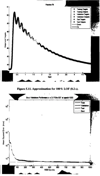
Figure 4.9. 100% LOF for 0.2 s 60 Figure 4.10. 100% LOF for 0.5 s 61 Figure 4.11. 100% LOF for 1 s 61 Figure 4.12. 50% loss of DIT for 0.1 s 63 Figure 4.13. 100% loss of DIT for 0.1 s 63 Figure 4.14. 50% over-excitation of DIT for 0.1 s 64
Figure 4.15. 100% over-excitation of DIT for 0.1 s 64
Figure 4.16. 100% loss of DIT for 0.2 s 66 Figure 4.17. 100% loss of DIT for 0.5 s 66 Figure 4.18. 100% loss of DIT for 1 s 67
Figure 4.19. SC for 0.075 s 68 Figure 4.20. SC for 0.150 s 68 Figure 4.21. SC for 0.212 s (Marginally Stable) 69
Figure 4.22. SC for 0.213sec (Unstable) 69 Figure 4.23. Comparison of SC for 0.075 s, 0.150 s, 0.212 s (Marginally Stable) & 0.213sec
(Unstable) 70 Figure 5.1. Approximation in blue and actual signal in red (a) log(x) (b) exp(x) 74
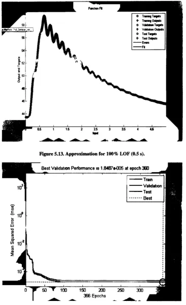
Figure 5 13 Approximation for 100% LOF (0 5 s) 85 Figure 5 14 Error curve for 100% LOF (0 5 s) 85 Figure 5 15 Approximation for 100% LOF (Is) 86 Figure 5 16 Error curve for 100% LOF (Is) 86 Figure 5 17 Approximation for 50% loss in DIT (0 1 s) 88
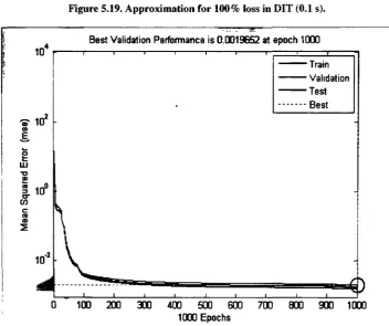
Figure 5 18 Error curve for 50% loss m DIT (0 1 s) 88 Figure 5 19 Approximation for 100% loss in DIT (0 1 s) 89 Figure 5 20 Error curve for 100% loss in DIT (0 1 s) 89 Figure 5 21 Approximation for 50% over-excitation in DIT (0 1 s) 90
Figure 5 22 Error curve for 50% over-excitation in DIT (0 1 s) 90 Figure 5 23 Approximation for 100% over-excitation in DIT (0 1s) 91 Figure 5 24 Error curve for 100% over-excitation in DIT (0 1s) 91 Figure 5 25 Approximation for 100% loss in DIT (0 2 s) 92 Figure 5 26 Error curve for 100% loss in DIT (0 2 s) 93 Figure 5 27 Approximation for 100% loss in DIT (0 5 s) 93 Figure 5 28 Error curve for 100% loss in DIT (0 5 s) 94 Figure 5 29 Approximation for 100% loss in DIT (Is) 94 Figure 5 30 Error curve for 100% loss in DIT (1 s) 95 Figure 5 31 Approximation for SC for 0 075 s 96 Figure 5 32 Error curve for SC for 0 075 s 97 Figure 5 33 Approximation for SC for 0 150 s 97 Figure 5 34 Error curve for SC for 0 150s 98 Figure 5 35 Approximation for SC for 0 212 s (Marginally Stable) 98
Figure 5 36 Error curve for SC for 0 212 s (Marginally Stable) 99
Figure 6 1 SOM weight plane 106 Figure 6 2 SOM neighbor weight distances 107
LIST OF TABLES
Table 4.1. Machine parameters 51 Table 4.2. Operating conditions 51 Table 5.1. Neural network 76 Table 5.2. Neural network specification 76
Table 5.3. Neural network training conditions 77
Table 6.1. Neural network 104 Table 6.2. Neural network specification 104
Table 6.3. Neural network specification 105
Table 7.1. Neural network 112 Table 7.2. Neural network specifications 113
Table 7.3. Neural network training conditions 114
Table 7.4. Neural network 115 Table 7.5. Neural network specifications 116
Table 7.6. Neural network training conditions 116
Table 7.7. Neural network 117 Table 7.8. Neural network specifications 118
Table 7.9. Neural network training conditions 118
Table 7.10. Neural network 119 Table 7.11. Neural network specifications 120
Table 7.12. Neural network training conditions 120
NOMENCLATURE
Generally symbols have been defined locally. The list of principle symbols is
given below.
Ra Stator winding resistance
Rkdi, Rkqi d- and q-axis 1st damper resistances
Rkd2, Rkq2 d- and q-axis 2nd damper resistances
Rfd, Rkqs Field and 3rd q-axis damper resistances
Lj, Lq d- and q-axis synchronous Inductances
Lkdi, Lkqi d- and q-axis 1st damper Inductances
Lkd2, ^2 d- and q-axis 2nd damper Inductances
Lfd, ^3 Field and q-axis 3rd damper Inductances
1 INTRODUCTION
1.1 Background
The synchronous machine has long been the most important of the
electromechanical power-conversion devices, playing a key role both in the production of
electricity and in certain special drive applications. The history of the synchronous
machine is now more than 100 years old. Within this span of time its power capacity has
grown enormously, and it has established itself as a major player in the conversion of
energy. Its beginnings are found in the closing decades of the 1800s, when innovatory
engineers in several different countries showed courage, conviction and far-sightedness
as they worked on its early development.
The beginning was in the 1880s. At first, stationary poles were used, with the
poles surrounding a rotating ring armature. This was known as the external-pole type. An
important milestone was the 'three-phase dynamo' derived from the direct-current
machine with the Thomson-Houston armature. In 1887. the first three-phase synchronous
generator shown in Figure 1.1 was built, which produced about 2.8 kW at 960 rev/min.
corresponding to a frequency of 32 Hz.
1891 was the year in which the three-phase synchronous machine passed its first
big test and made its actual breakthrough. The scene was the Frankfurt Exposition, the
event the great experiment whereby 300 hp was transmitted from the hydroelectric power
plant at Lauffenam Neckar, 175km away, via three-phase current transmission. It was an
event that drew worldwide attention and acclaim. The appearances of powerful steam
turbines are at about the beginning of the 20th century. In 1901, the first actual
turbogenerator was built by Charles E. Brown [1].
We have to thank the Americans for building the first hydrogen-cooled machines.
They started in 1928 with a synchronous compensator, and in 1936 they put the first
3,600 rev/min hydrogen-cooled turbogenerator into commercial operation [1]. The first
hydrogen-cooled turbine generator developed by the GE Company went into service in
1937, and hydrogen-cooled machines were able to satisfy the power output needs for
many years. Between 1950 and 1960, manufacturers developed a broad range of direct
cooling methods.
A milestone of the 1970s was the appearance of superconducting (SC)
synchronous generator technology. A prototype of two-pole "utilitytype" generator was
built during the early 1970s using low temperature superconducting (LTS) wires. A
5-MVA generator was developed and successfully tested in 1972. The purpose of these
activities was to assess the technical feasibility of SC generators for long-term reliable
operation on electric power systems. In 1979 a 20 MVA two-pole 3,600 r/min turbine
generator for utility applications was designed, built, and load tested which was the
largest SC generator to be fully load tested.
This LTS conductor technology was used in the design of an SC rotor for a
synchronous turbo-generator. This rotor was essentially designed as a 250 MW machine
with an active length of 2 m and an overall length of 3 m, but used a larger diameter of a
1200-MW machine (1.06 m) [2].
Great improvements of computers mark the 90's; powerful softwares were
developed to design and analyze the synchronous generators. In 1995, K.W. Cowan
presented advanced computational techniques involving computational fluid dynamics
performance of prototype hydrogen cooled generator. During the last years of 1990s, the
SuperGM project, which was launched by the Japan New Energy and Industrial
Technology Development Organization in 1988, resulted in three models of
superconducting rotors and a conventional stator. Between October 1998 and June 1999,
this model machine was connected to a commercial power grid for the first time in the
world to study basic performance in an actual electric power system.
Application of high temperature superconducting (HTS) materials in synchronous
generators was a great milestone in this technology. In the mid-1990s, GE conducted
design studies on HTS generators and built and tested an HTS prototype coil [2]. Last
years of 1990s encountered the appearance of the powerformer technology. The idea of
electrical generation in high voltages was proposed in the beginning of 1998 by Dr Mats
Leijon from the ABB Corporate Research in Sweden. A new type of generator offered a
possibility to build high voltage generators, which could be directly connected to the
power transmission systems without any step-up transformer. In 1998, the first
powerformer was installed in the Porjus power plant in the north of Sweden with the
rating voltage of 45 kV and the rating power of 11 MVA [3].
Synchronous generators form the principal source of electric energy in power
systems. Many large loads are driven by synchronous motors. Synchronous condensers
are sometimes used as a means of providing reactive power compensation and controlling
voltage. These devices operate on the same principle and are collectively referred to as
synchronous machines. The power system stability problem is largely one of keeping
interconnected synchronous machines in synchronism. Therefore, an understanding of
their characteristics and accurate modeling of their dynamic performance are of
fundamental importance to the study of power system stability.
The modeling and analysis of the synchronous machine has always been a
challenge. The problem was worked on intensely in 1920s and 1930s [4]. [5] and has
been the subject of several more recent investigations [5]. [7]. The theory and
performance of synchronous machines have also been covered in a number of books [8],
Synchronous machines while generating power are usually connected to a grid.
As one of the prime requirements of synchronous machines is to run them in synchronous
speed, as any distortion from synchronism can lead to instability of the grid i.e. the
system. Synchronous machines while operating in generation mode are subjected to
different kinds of faults or disturbances which can lead to potential speed distortion and
ultimately instability of the system. To prevent this there are different kinds of precaution
that have been taken. A lot of these precautions invohe implementation of protection
relays which depends on fault detection and analysis.
Nowadays, to connect a synchronous machine to a system for testing purposes are
not so practical. Same goes for analyzing and investigating it for fault detection for the
enormity and complexity of the machines as well as the complexity of the power system
and the importance of its stability. With the rapid and vast development of computer
based analysis tools the solution has to come as a package where the system is already
analyzed the outcome is expected. In the field of fault detection there are different kinds
of common occurrences in faults under which the machine behaviors should be analyzed
and possible solution should be in effect. Of the faults very common occurrences are loss
of field or excitation, disturbances in input torque, short circuit faults etc. For the sake of
power system stability is absolutely nonnegotiable to have a proper understanding of how
a machine going to behave under any of the faults and as well to identify what kind of
fault is in incidence.
For the purpose synchronous machine computer aided analysis is done by
simulating synchronous machine models and observing its dynamic behavior if different
kinds of fault is initiated. It is also of utmost importance to detect what kind of fault is in
occurrence by just looking at the machine activities. Under certain situation if there are
multiple fault occurrences it is also essential to filter different kinds of faults to
distinguish and identify them.
Up to the point different type of synchronous machine models are in effect, which
are good approximations of the actual system. They are at most of the cases being
machine model solution. Fault detection and distinguishing can be tricky under certain
situations where fault specific behaviors are not very well known.
1.2 Research Objectives
The objective of this research is to understand and realize synchronous machine
dynamic performances and to propose and design a better modeling of synchronous
machine for the purpose; to understand behavior of synchronous machine performance
under different kinds of fault and study system stability under these conditions; to
identify and to be able to distinguish between different kinds of faults.
In this research work, artificial neural network has been used as a tool for the
purpose:
> For approximation and characterization of synchronous machine dynamic
behavior under different fault conditions
> For fault distinguishing and filtering under mixed or multiple fault occurrence
> For fault detection and identification to various details by looking at machine
behavior
To achieve these purposes neural network based characterization, clustering and pattern
recognition has been used.
1.3 Thesis Outline
This thesis is organized as follows:
Chapter 2: In this chapter, synchronous machine and its model details is being defined. Here synchronous machine is described from its operational point
of view, constructional point of view and other theories related to it.
Synchronous machine mathematical model is being depicted which is later
used in chapter 4 for simulation purposes.
Chapter 3: Artificial neural network with its understanding and different aspects is focus of the chapter. Special types of artificial neural networks and there
attributes being scrutinized to comprehend there implicational and
contextual properties.
Chapter 4: Synchronous machine model described in chapter 2 is simulated and
dynamic analysis is performed. Simulation and result from the simulation
is presented with detailed description and explanation.
Chapter 5: In this chapter, neural network characterization is used to approximate synchronous machine model using neural networks. The simulation of the
approximation is presented under various dynamic conditions.
Chapter 6: In this chapter, neural network clustering is used to filter and distinguish between different kinds of faults in the case of multiple fault situations.
The simulation results are presented.
Chapter 7: In this chapter, neural network pattern recognition technique is used to detect faults by looking at machine behaviors. Fault detection is done
between different kinds and levels of faults. The simulations and findings
are presented in end of the chapter.
Chapter 8: Findings of this research work is summarized in this chapter.
1.4 References
[1] G. Neidhofer, "The evolution of the synchronous machine," Engineering
Science and Education Journal, pp. 239-248, October 1992.
[2] S. Kalsi, K. Weeber, H. Takesue, C. Lewis, "Development status of rotating
machines employing superconducting field windings," Proceeding of the IEEE.
vol. 92, no. 10, pp. 1688-1704, October 2004.
[3] M. Leijon, M. Dahlgren, L. Walfridsson, L. Ming and A. Jaksts, "A recent
development in the electrical insulation systems of generators and transformers,"
IEEE Electrical Insulation Magazine, vol. 17. no. 3, pp. 10-15, May/June 2001.
[4] R.H. Park, "Two-Reaction Theory of Synchronous Machines - Generalized
[5] R.H. Park, "Two-Reaction Theory of Synchronous Machines - Part II," AIEE
Trans., vol. 52, pp. 352-355, 1933.
[6] G. Shackshaft and P.B. Henser. "Model of Generator Saturation for Use in
Power System Studies," Proc. IEE (London), vol. 126, no. 8, pp. 759-763. 1979.
[7] EPRI Report EL-3359, "Improvement in Accuracy of Prediction of Electrical
Machine Constants, and Generator Model for Subsynchronous Resonance
Conditions," Final Report of EPRI Projects RP 1288-1 and RP. vols. 1, 2 and 3.
(Prepared by General Electric Company), 1984.
[8] E.W Kimbark, Power System Stability, Vol. Ill: Synchronous Machines. John
Wiley & Sons, 1956.
[9] A.E. Fitzgerald and C. Kingsley, Electric Machinery, Second Edition,
McGraw-Hill, 1961.
2 S Y N C H R O N O U S M A C H I N E MODELING
2.1 Introduction
Synchronous machine is the most used machine in the purpose of electric power
generation in the world. That is most of the energy com ersion where mechanical power
is converted into electrical power, large scale s\nchronous machine are in use. It's an AC
machine where the rotor of the machine is in synchronism with the rotating stator
magnetic field which refers its being in synchronism to the electrical frequency.
To understand the modeling of machine one has to understand a machine's
construction, the fundamentals it operates on, mathematical model etc. To be able to
analyze a machine one have to realize their underlying relationships. In the next section
the key aspects of synchronous machine is portrayed and an effort was made to interrelate
them. Also a synchronous machine mathematical model is described which is developed
based on a standard IEEE model [1].
2.2 Theory and Modeling of Synchronous Machine
2.2.1 Constructional features
From mechanical point of view a synchronous machine has basically two parts:
stator and rotor. The stator is the stationary part which has a three phase winding which is
spatially distributed and either Y-connected or A-connected. Stator in a synchronous
machine is the armature as the larger current flows through it. The rotor is the rotating
part of the machine which has a DC winding. That is a DC power supply powers the rotor
to make it act as an electromagnet. Hence, the rotor in a synchronous machine is the field
[2]-2.2.2 Operating principles
Synchronous machine is an electromechanical energy conversion unit, which can
convert mechanical energy to electrical and electrical energy to mechanical. When it
converts electrical energy to mechanical energy it is said to be operating in motoring
mode shown in Figure 2.1(a) and when it is converting mechanical energy to electrical it
is called to be operating in generating mode shown in Figure 2.1(b). In most of the cases
they are used as generators because of their high efficiency.
To understand the operating principles of synchronous machine it is assumed that
the machine is operating in motoring mode. Once understood the motoring mode the
generating mode works in the same way. except the direction of the operation is
completely opposite. In motoring mode, a three phase AC power is supplied as in Figure
2.2. The three phase power supply creates a rotating magnetic field. The speed of the
rotating magnetic field is synchronous to the frequency of the AC power supply and the
speed depends on the number of poles in the rotor. As the electrical frequency and the
number of poles in a synchronous machine are constant, the speed is as well [2]. The
speed of the magnetic field can be calculated as,
• .1 r' ^
(a) (b)
Figure 2.1. Synchronous machine operation, (a) Motoring mode (b) Generating mode.
Figure 2.2. Three-phase AC signal.
St
Figure 2.3. Field winding in the rotor.
(2.1)
Where,
is the electrical frequency in per second (Hz)
P is the number of poles
N is the synchronous speed in revolution per minute (rpm)
The DC power supply in the rotor winding as in Figure 2.3 makes the rotor act as
an electromagnet; hence the magnetic field is created. The rotating magnetic field in the
stator circuit cuts the magnetic field from that field winding of the stator; as a result they
try to align with each other. As the rotating magnetic field continuous to rotate the rotor
(g) (h) (i) 0) (k) (1)
Figure 2.4. Rotating magnetic field of a synchronous machine.
(g) (h) (i) ()) (k) (1)
Figure 2.5. Synchronous machine rotation.
Rotation of the magnetic field in the stator circuit is shown in Figure 2.4(a)-(l).
The rotation of the rotor because of the electromagnetic induction is shown in Figure
2.5(a)-(l). It is evident from the Figures 4 and 5 that the rotation of synchronous machine
2.2.3 Reference frame theorem
The understanding of synchronous machine mathematical model one needs to
have a proper understanding of reference frame theorem. Before getting in to the details
of the reference frame theorem of a synchronous machine let us look at the machine
equations from organizational point of view. From one point of view the mathematical
model has two basic sets of equation describing the whole model - the electrical
equations and the mechanical equations.
Now looking at the electrical part of the machine, the model as per machine
structural construction has two distinct parts - the rotor and stator, thus, a set of equations
that describes the stator part and another set of equations that describes the rotor part.
Since, the rotor and stator of the machine are linked through magnetic flux while
operating, the equations describing both stator and rotor are interconnected.
In describing the mathematical model problem arises as the stator is stationary
and the rotor is rotating, and one has to inter-link the equation to make sense out of them;
which calls for taking either stator or rotor as reference. In describing these equations
whether the rotor or the stator or any other variable is taken as a reference is realized is
expressed through reference frame theory.
^ d-axis
Like many other coordinate system the reference frame theory is primarily defined
by two axes as shown in Figure 2.6: direct and quadrature axes. All the vectors in the
mathematical model of a synchronous machine are dissolved to these two axes. So, as in
Figure 2.6, if an arbitrary vector X is assumed with an angle 9 with respect to direct axis,
it will have to be dissolved in two components - the d-axis component: Xd = X cosG and
the q-axis component: Xq = X sin9. All the vectors in the space which describe the machine operation are thus resolved into d and q axis components.
2.2.4 Per unit system
A per-unit system is the expression of system quantities as fractions of a defined
base unit quantity. Calculations are simplified because quantities expressed as per-unit
are the same regardless of the voltage level. Similar types of apparatus will have
impedances, voltage drops and losses that are the same when expressed as a per-unit
fraction of the equipment rating, even if the unit size varies widely. Conversion of
per-unit quantities to volts, ohms, or amperes requires knowledge of the base that the per-per-unit
quantities were referenced to.
A per-unit system provides units for power, voltage, current, impedance, and
admittance. Only two of these are independent, usually power and voltage. All quantities
are specified as multiples of selected base values. Per unit system is a way of normalizing
machine parameters so that one can make a comparison between machines with different
specification. In this research work all the values are calculated in per unit system [3].
Actual value Per unit value = — ;
Base value
2.3 Mathematical Modeling
Mathematical model of a machine is realizing the machine in terms of a set of
differential equation and polynomials. To understand a machine model and to relate and
realize the relationship between the machine constructions, their broken down parts,
operating principles and how the electrical and the mechanical vectors and variables in
same story using different point of views. This includes the circuit diagram, machine
equations, phasor diagram etc. In this model synchronous reference frame is used to
depict the machine equations.
2.3.1 d-axis mathematical modeling
The d-axis circuit diagram of the synchronous machine model is shown in Figure
2.7 which describes the d-axis electrical model [1], [2]. In this model, one field winding
and two damper windings are considered in d-axis rotor circuit. The machine is assumed
to be in a generation mode. All the currents in the machine should be assumed in an
outward direction that is anti clockwise in the loops.
Looking at the circuit diagram to describe the relationship two sets of equations is
being used. The first set are the voltage equations, which are differential equations
relating voltage and flux. The second set of equations is flux equations which relates
current and flux. The first equation in each set represents to the stator electrical model
and the later three the rotor electrical model. The second equation in each set is
representing the field circuit and the later two the damper circuit.
+A
Ra U>r¥q Ll Lfld-Lad
Jc
+
PVd
v _
\L ad T +
'Id \L 2d
P¥ld%Rld P¥2d^R2d
+A
twv^O^w-_ *
PWa
v _
k.
•lq
7 T T
I , .
PVl^
Rlq PW2^
RZq
'-*?
/J, ^ *
Voltage equations:
Flux equations:
Figure 2.8. q-axis circuit diagram.
efd=Rfdifd+PVfd o = Ruhd + pvld
0 = Rldha + PVld
Vd = (Lad + Ll h "" Ladtfd - Ladhd
Wfd = Lra\fd + LJ irf'lj - Ladld
^\d ~ L/\d'fd +L\)dhd ~^ad'd
V2a ~ ^fld'fd + Lzidhd ~ ^ad'd
(2.2)
(2.3)
23.2 q-axis mathematical modeling
The q-axis circuit diagram of the s)rnchronous machine model is shown in Figure
2.8 which describes the q-axis electrical model [1]. [2]. In this model, three damper
windings are considered in q-axis rotor circuit. The machine is assumed to be in a
generation mode. Looking at the circuit diagram to describe the relationship t\\ o sets of
equations is being used. The first set are the voltage equations, which are differential
equations relating voltage and flux. The second set of equations is flux equations which
relates current and flux. The first equation in each set represents to the stator electrical
Voltage equations:
Flux equations:
Q = R\qi\q+PV\q
^ = R2qi2q+P^>2q
0 = R3qhq + PViq
Vq = {La„ + L,)i„ + Laqhq + Laqhq
¥xq = Lnqhq + Laq(hq + »3, J " Laq'q
W2q = LaA, + i,,)+ LnL - Li
Viq=L<l+i2Q) + L2 - LJ
(2.4)
(2.5)
2.3.3 Steady-state operation
The phasor diagram of a synchronous machine shows the relationship of
synchronous machine voltage and current with the phase differences. It is necessarily
useful for realizing the steady state condition of a synchronous machine, which is used as
an initial condition of the machine simulation. From the voltage diagram in Figure 2.9,
d-and q-axis terminal voltages can be found which later are being used to calculate the load
angle [4], [5]. The load angle is used to calculate the initial conditions for machine
operation.
..•• q-axrs
•>J d-axis
-W-
•o£,ZOc0
E
*
ZS
>
Figure 2.10. Simplified circuit diagram.
Calculation of load angle:
Vd=Vtsmb,Vq=Vtcosh
5 = tan /, .Lq. cos 9 - /, .Ra. sin 0
Vt +IrLrsmQ + IrRa.cos6
(2.6)
Where, ©0 = 2nf, f = 60 Hz, p
dt
2.3.4 Mechanical equations
The mechanical part of the mathematical model describes the mechanical
phenomenon of the machine as well as relates the mechanical effect with speed and load
angle. As the electrical model of the machine depends on load angle and speed to
calculate different parameters, the load angle and the speed are the relating factor
between mechanical and electrical model.
d8
— = COnAO),
dt W
^ = -L(r
-T)
dt 2HKm e).
2.3.5 Current flux relationship in matrix form
Another way of looking at machine equations is a matrix form. Matrix form is just
manipulation of the existing equations and representing in terms of matrix multiplication
[6]. This is especially useful when programs are written in the purpose of numerical
simulation. In matrix form the whole model is portrayed in three distinct matrixes; the
current, flux and inductance matrix:
Where:
1 = L 1y
I ~ Vd *kd\ ikdl ifd *q %\ ikql *kq3 \
H> = [Vd Vkd\ Vkdl Vfd Vkq\ Vkql M>fc,3 f
(2.8)
Lmd umd
~Lmd hnd+Lkd Lmd Lmd
Lmd 0
-L, 'md Lmd 0 0 0 0 Lmd Lmd 0 0 0 0
Lmd+LkdL Lmd °
Lmd Lmd+Lfd ° °
" ~Lq hnq
0 -Lmq Lmq+Lk4
0 0 0 0 ^mq X, mq 0 0 0 0 hnq *-Tnq
hnq hnq hnq+^kql hnq
~hnq hnq hnq hnq+hkqi
2.3.6 Internal control system
Synchronous generators are usually connected to the grid. This means that they
have constant terminal voltage with a specific loading condition. While synchronous
machine is operating under a grid it is usually generating power while running in
synchronous speed. It is important to understand that synchronism in speed of a
synchronous machine is a requirement, as any distortion in synchronism can lead to
disturbance it usually gives away its extra kinetic energy as electrical energy to the grid
and tends to comes back to synchronous speed. On the other hand, if it goes to a
sub-synchronous speed, it absorbs some of the electrical energy and tends to speed up to go to
the synchronous speed [2]. This tendency of synchronous machine to operate in
synchronous speed is can be views as the internal control system which is shown in
Figure 2.11. The control equations are:
COnA, A . J0-,N
T =^ofnt C0„
(2.9)
(2.10)
2.4 Saturation
Saturation is one of the most common occurrences in the nature; it is also true for
electric machines with no exception in synchronous machines. It has been seen that
taking saturation into account gives more accurate and realistic results [7], [8]. Two
models of synchronous machine are developed in this research work. In the first model
saturation is ignored and in the second model it's taken into account.
M a c h i n e M o d e l
2.4.1 Unsaturated model
In the unsaturated mode the d-axis saturation and the q-axis saturation ignored,
that is the d- and q-axis magnetizing reactances, Xm(j and Xmq. are assumed to be equal to their unsaturated values.
2.4.2 Saturated model
In electric machines, saturation is of basic two kinds: leakage flux saturation and
main flux saturation.
2.4.2.1 Leakage flux saturation
Leakage flux saturation is defined by the saturation in the leakage flux of a
machine. In this research work the leakage flux saturation is ignored. This is because it
has negligible effect on the machine performance in comparison to the machine main flux
saturation.
2.4.2.2 Main flux saturation
In this case, both d- and q-axis saturation are considered. The unsaturated d- and
q-axis magnetizing reactances are replaced by their corresponding saturated values.
These d- and q-axis saturated magnetizing reactances, X^ and Xmqs, are obtained by modifying the corresponding unsaturated values, Xmdu and XmgU, with two saturation factors calculated from the polynomials fitting the saturation curves. The d- and q-axis
magnetizing ampere-turns {ATa, ATq) are used to locate the operating points on the d- and q-axis saturation characteristics respectively [9]-[ll].
By applying the procedure described above, the transient performance of
synchronous machines considering the saturation along the direct and quadrature axes
can be calculated. However, in this case, an iterative technique has to be applied to
determine the transient performance as the saturated d- and q-axis magnetizing reactances
d-axis saturation
\yds = f(ATd) = -0.1501 AT] +0.03S3 AT] +1.0283 ATd -0.0007
X = v*
mds irp
A1d (2.11)
q-axis saturation
V = j\AT) = - 0 . 0 1 5 5 A Tqs 3- 0 . 2 2 4 6 A T2 +1.066AT -0.0012
Vqs X —
i (2.12)
2.5 Rotor Angle
The electrical angular displacement of the rotor relative to its terminal is defined
as the rotor angle. The rotor angle is the displacement of the rotor generally referenced to
the maximum positive value of the fundamental component of the terminal voltage.
Therefore, the rotor angle expressed in radian is,
6 = 9r- 9e (2.13)
Where,
9r is the rotor angle
6eis the angle of electrical magnetic field
Speed (GO) of a synchronous machine can be found by differentiating 9; hence any
disturbance in the speed of the machine can be interpreted as change in 8. In steady state
condition the speed of a synchronous machine is a constant. As a result 8 is constant. Any
change in speed in the machine thus can be interpreted from change in 8.
In this research work, in disturbance introduced in the machine is realized by
looking at 8 as an output. Regardless of what the disturbance is, how much the machine is
affected and how much the stability of the machine is disturbed is analyzed and
2.6 References
[I] IEEE Guide for Synchronous Generator Modeling Practices in Stability
Analyses, Std. 1110-1991.
[2] P Kundur, Power System Stability and Control, McGraw Hill, 2004.
[3] A.E.Fitzgerald, C. Kingsley, and S.D. Umans, Electric Machinery.
McGraw-Hill, 1991.
[4] L. Wang; J. Jatskevich, and H.W. Dommel, "Re-examination of synchronous
machine modeling techniques for electromagnetic transient simulations," IEEE
Transactions on Power Systems, vol. 22. no. 3, pp. 1221 - 1230, Aug. 2007.
[5] M. Kakiuchi, S. Nagano, D. Hiramatsu, K. Koyanagi. K. Hirayama, Y. Uemura,
T. Satoh, and K. Nagasaka, "A study of synchronous machine modeling about
synchronizing phenomena," IEEE International Conference on Electric
Machines and Drives, pp. 890 - 895. 15-15 May 2005.
[6] C. Ellis, H. Nouri, R. Ciric, and B. Miedzinsky, "Overview of the development,
simplification and numerical analysis of synchronous machine models for
stability studies," 42" International Universities Power Engineering
Conference, pp. 1019 - 1023, 4-6 Sept. 2007
[7] N.C. Kar and A.M. El-Serafi, "Effect of the main flux saturation on the transient
short-circuit performance of synchronous machines,"' IEEE Canadian
Conference on Electrical and Computer Engineering, pp.629 - 632, May 1-4,
2005.
[8] A.M. El-Serafi and A.S. Abdallah. "Saturated synchronous reactances of
synchronous machines," IEEE Transactions on Energy Conversion, vol.7, no. 3.
pp.570 - 579, Sept. 1992.
[9] F.P. Mello, "Representation of saturation in synchronous machines," IEEE
Trans, on Power Engineering Society, vol. PWRS-1, no. 4, p.8, 1986.
[10] E. Levi, "Modeling of magnetic saturation in smooth air-gap synchronous
machine," IEEE Trans, on Energy conversion, Vol. 12, no. 2. pp. 151-156, June
1997.
representing saturation in physical variable models of synchronous machines",
IEEE Trans, on energy conversion, vol.14, no. 1, pp. 72-79, March 1999.
[12] D. Hiramatsu, K. Hirayama, T. Tokumasu, Y. Uemura, M. Takabatake, Y
Ishikawa, and A. Iwai, "Analysis of damper saturation characteristic on
synchronous machine transient condition," IEEE Power Engineering Society
3 ARTIFICIAL N E U R A L N E T W O R K (ANN)
3.1 Introduction
An artificial neural network (ANN) as shown in Figure 3.1, often just called a
"neural network" (NN), is a mathematical model or computational model based on
biological neural networks. It attempts to simulate the structure, interconnections and
interactions of the nerve cells of a biological brain, while have the capability to update its
knowledge from experience. It consists of an interconnected group of artificial neurons
and processes information using a connectionist approach to computation. In most cases
an ANN is an adaptive system that changes its structure based on external or internal
information that flows through the network during the learning phase.
In more practical terms neural networks are non-linear statistical data modeling
tools. They can be used to model complex relationships between inputs and outputs or to
find patterns in data.
Neural network as an idea comes from observing central nervous system and its
construction. The neurons in central nervous system along with their axons, dendrites and
synapses constitutes for the most sophisticated information processing entity. In a neural
network model, replicating the central nervous system, simple nodes called "neurons",
"neurodes", "PEs" ("processing elements") or "units" are connected together to form a
network of nodes. Hence it is called "neural network" These neural networks of simple
processing elements (neurons), can exhibit complex global behavior, whereas its
complexity and capability is determined by the number of connections, connections
paradigm between the processing elements, and element parameters. The practical use of
a neural network comes with algorithms designed to alter the strength (weights) of the
connections in the network to produce a desired signal flow [l]-[4].
Even though, in the crams of theoretical neuroscience neural networks models are
designed with an intention to emulate that of a central nervous system (CNS), artificial
neural network as a term in concurrency is a subject to utilization to design models in
Input Layer
'V-*/
•i Hidden Layer
±^^^r^ "^H^g^ ^ ^ ^ ^ ^
-L
"i-Output Layer
>o—
V;
# :
Figure 3.1. Artificial Neural Network (ANN).
Devoid of any qualm, biology has inspirited the invention of artificial neural
network. In modern numerical implementation the approach is more or less discarded to
fit the practical implicational needs based on signal processing and statistics. Both
adaptive and non-adaptive elements are considered as used to realize large systems;
though adaptive approach is more contextual in practical implementation which has a
basis of non-linearity, distribution, parallelism, and local processing and adaptation.
3.2 Overview of ANN
3.2.1 Model
Artificial neural networks (ANNs) are in essence simple mathematical models
defining a function, f:X^>Y Any ANN model corresponds to a class of such functions.
Figure 3.3. Recurrent ANN dependency graph.
Figure 3.2 illustrates essentials of a fundamental network structure with arrows
depicting dependencies between variables, whereas_/[*) is defined as,
(3.1)
In this case f[x) is a composite of a function g,{x) which can be represented as a
simple vector,
It is a widely used type of composition known as the nonlinear weighted sum.
In similar fashion g,(x) can be shown as composite of other function depending on
the network structure.
Interpretation of dependencies of the variables indicated by the arrows can be
scrutinized in two ways, as in Figure 3.3 in case of function/
Functional view: Input x is transformed into a 3-dimensional vector h, which is
then transformed into a 2-dimensional vector g, which is finally transformed into/ This
view is most commonly encountered in the context of optimization.
Probabilistic view: Random variable F = fiG) depends upon the random variable G = g(H), which depends upon H = h(X), which depends upon the random variable X.
This view is most commonly encountered in the context of graphical models.
Either of the views while implementation accord, has a naturally inhabited
capability of enabling parallelism in some extent, which refers to the fact of them being
independent of their inherited variables, hence, more or less equivalent quite to an extent;
The network with acyclic configuration in Figure 3.2 is usually known as
feedforward neural network and the one with cyclic organization in Figure 3.3 is known
as recurrent neural network [4]-[7].
3.2.2 Learning
No matter how interesting a neural network is with functions defining its
structural paradigm, the most intriguing and captivating possibility lies in its
competencies in learning ability [8]. Learning implementing a neural network optimally
by observation means, given a specific task to solve a class of functions F, in order to
find fe F.
This entails defining a cost function which is defined by C: F -> M such that, for
the optimal solution/*,
C(/*) < C(f)Vf E F (3.2)
That is, no solution has a cost less than the cost of the optimal solution.
Cost function C is an evaluation process through which it can determined to what
extent a network is successful to learn a problem, in other words, how far the network is
from the optimal solution of the problem dataset it is suppose to learn. The learning
algorithm searches through the solution space with the intention of finding that of a
smallest possible cost as appropriate.
For applications where the solution is dependent on some data, the cost must
necessarily be a function of the observations; otherwise we would not be modeling
anything related to the data. It is frequently defined as a statistic to which only
approximations can be made. As a simple example considering the problem of finding the
model/which minimizes C as, C = E[(f(x) — y)2] for data pairs (xj/) drawn from some distribution!).
In practical situations, TV samples from T) will be available and thus, for the above
example, we would only minimize, C = -££Li(/(*f) - y*)2 Thus, the cost is
For online learning parameter N -» oo; as the learning progresses through time,
the cost function is partially minimized with ingression of new data. Online learning is
often used when T) is fixed. In the case of finite dataset various customized versions of
online learning are often being used [9], [10].
The use of problem specific cost functions is a frequent practice, although
assigning ad hoc cost function in an arbitrary fashion can do the job. Obviously choosing
problem specific cost function has its advantages in terms if addressing problem specific
approximation; i.e. convexity in a model or probabilistic formulation the posterior
probability of the model used as an inverse cost. In the end, choice of cost function is
coherent to the task.
3.2.3 Learning paradigms
There are three major learning paradigms, for any given type of network
architecture, each corresponding to a particular abstract learning task:
• Supervised learning
• Unsupervised learning
• Reinforcement learning.
3.2.3.1 Supervised learning
In supervised learning, a given set of example pair is (x,y), where x E X,y 6 Y
and the aim is to find a function f:X -> Y in the allowed class of functions that matches
the examples. In other words, it is inferred that the mapping is implied by the data; the
cost function is related to the mismatch between the mapping and the data and it
implicitly contains prior knowledge about the problem domain.
A commonly used cost is the mean-squared error which tries to minimize the
average squared error between the network's output, fix), and the target value y over all
the example pairs. When one tries to minimize this cost using gradient descent for the
class of neural networks called Multi-Layer Perceptrons, one obtains the common and
Pattern recognition (also known as classification) and regression (also known as
function approximation) are the tasks which fall under the paradigm of supervised
learning. The supervised learning paradigm is also applicable to sequential data (e.g., for
speech and gesture recognition). This occurs in the form of a function that provides
continuous feedback on the quality of solutions obtained up to that point [11].
3.2.3.2 Unsupervised learning
In unsupervised learning, some data x is given, and the cost function to be
minimized can be any function of the data x and the network's output,/ The cost function
is dependent on the task and as a priori assumption. For example, considering a model
fix) = a, where a is a constant and the cost C = E[(x -fix))2]. Minimizing this cost will give a value of that is equal to the mean of the data. The cost function can be in a form
dependent on the application: In compression it could be related to the mutual
information between JC and y. In statistical modeling, it could be related to the posterior
probability of the model given the data [12], [13].
Tasks that fall within the paradigm of unsupervised learning are in general
estimation problems; the applications include clustering, the estimation of statistical
distributions, compression and filtering [14].
3.2.3.3 Reinforcement learning
In reinforcement learning, data x is usually not given, but generated by an agent's
interactions with the environment. At each point in time t, the agent performs an action yt
and the environment generates an observation x, and an instantaneous cost C,, according
to some dynamics. The aim is to discover a policy for selecting actions that minimizes
some measure of a long-term cost, i.e. the expected cumulative cost. The environment's
dynamics and the long-term cost for each policy are usually unknown, but can be
estimated.
More formally, the environment is modeled as a Markov decision process (MDP)
with states s1,...,snEs and actions a1; . . . , amE a with the following probability
distributions: the instantaneous cost distribution P(ct\s,), the observation distribution
distribution over actions gi\en the observations. Taken together, the two define a Marko\
chain (MC). The aim is to discover the polic> that minimizes the cost. i.e. the MC for
which the cost is minimal.
ANNs are frequenth used in reinforcement learning as part of the o\erall
algorithm. Tasks that fall within the paradigm of reinforcement learning are control
problems, games and other sequential decision making tasks.
3.2.4 Learning algorithms
Most of the training algorithms can be scrutinized as a fundamental use of
optimization theory statistical estimation. Presently there are numerous optimization
algorithms are available for training a neural network, whereas choosing a model implies
to selection of one from a set of allowed one, criteria being minimization of the cost
function.
Gradient descent algorithm is a widespread tactics used when it comes to train an
artificial neural network. In this method the derivath e of the cost function with respect to
the network parameters are considered and the change is done to those parameters in
accordance with gradient-related direction. Among the other frequently used method
evolutionary methods, simulated annealing and expectation-maximization and
non-parametric methods are common!} used methods for training neural networks. Temporal
perceptual learning relies on finding temporal relationships in sensory signal streams In
an environment, statistically, salient temporal correlations can be found by monitoring the
arrival times of sensory signals. This is done by the perceptual networks [6]. [9].
3.3 Real Life Applications
The utility of artificial neural network models lies in the fact that they can be used
to infer a function from observations. This is particularly useful in applications where
3.3.1 Applications of artificial neural networks
One of the most powerful applications of neural networks is function
approximation, or regression analysis. Time series prediction and system modeling are
typical examples of approximations or regressions. Classification is another popular
neural network application paradigm. Pattern recognition, sequence recognition, novelty
detection and sequential decision making are common type of classification example.
In the field of data processing neural networks are also used for various
application processes. Typical data processing application are filtering, clustering, blind
source separation and compression.
3.3.2 Application areas of artificial neural networks commonly spotted
Neural networks are applied in various fields to address different problems.
Commonly spotted application areas of artificial neural networks are observed in system
identification and control i.e. vehicle control, process control etc.; game-playing and
decision making i.e. backgammon, chess, racing etc; pattern recognition i.e. radar
systems, face identification, object recognition etc.; sequence recognition i.e. gesture,
speech, handwritten text recognition etc.; medical diagnosis; financial applications i.e.
automated trading systems; data mining i.e. knowledge discovery in databases ("KDD");
visualization; e-mail spam filtering; and many others.
3.4 Types of Neural Networks
3.4.1 Feedforward neural network
A feedforward neural network is an artificial neural network where connections
between the units do not form a directed cycle. In this network, the information moves in
only one direction, forward, from the input nodes, through the hidden nodes (if any) and
to the output nodes. There are no cycles or loops in the network. In a feedforward
Inputs Output
Figure 3.4. Feedforward neural network.
3.4.1.1 Single-layer perceptron
The earliest kind of neural network is a single-layer perceptron network, which
consists of a single layer of output nodes; the inputs are fed directly to the outputs via a
series of weights. In this way it can be considered the simplest kind of feedforward
network. The sum of the products of the weights and the inputs is calculated in each
node, and if the value is above some threshold (typically 0) the neuron fires and takes the
activated value (typically 1); otherwise it takes the deactivated value (typically -1).
Neurons with this kind of activation function are also called artificial neurons or linear
threshold units. In the literature, the term perceptron often refers to networks consisting
of just one of these units. A similar neuron was described by Warren McCuIloch and
A perceptron can be created using any values for the activated and deactivated
states as long as the threshold value lies between the two. Most perceptrons have outputs
of 1 or -1 with a threshold of 0 and there is some evidence that such networks can be
trained more quickly than networks created from nodes with different activation and
deactivation values. Perceptrons can be trained by a simple learning algorithm that is
usually called the delta rule. It calculates the errors between calculated output and sample
output data, and uses this to create an adjustment to the weights, thus implementing a
form of gradient descent.
Single-unit perceptrons are only capable of learning linearly separable patterns; in
1969 in a famous monograph entitled Perceptrons Marvin Minsky and Seymour Papert
showed that it was impossible for a single-layer perceptron network to learn an XOR
function. They conjectured (incorrectly) that a similar result would hold for a multi-layer
perceptron network. Although a single threshold unit is quite limited in its computational
power, it has been shown that networks of parallel threshold units can approximate any
continuous function from a compact interval of the real numbers into the interval [-1,1].
A single-layer neural network can compute a continuous output instead of a step
function. A common choice is the so-called logistic function:
y = —^r (3-3)
With this choice, the single-layer network is identical to the logistic regression
model, widely used in statistical modeling. The logistic function is also known as the
sigmoid function. It has a continuous derivative, which allows it to be used in
backpropagation. This function is also preferred because its derivative is easily
calculated: y' = y{\ ~y) (times dfldX, in general form, according to the Chain Rule)
3.4.1.2 Multi-layer perceptron
This class of networks consists of multiple layers of computational units, usually
interconnected in a feedforward way. Each neuron in one layer has directed connections
to the neurons of the subsequent layer. In many applications the units of these networks