Flow Modeling through an Electro-statically Charged Monolith Filter

ABSTRACT

GIRISAN, VIVEK. Flow Modeling through an Electro-statically Charged Nano-Particle Filter. (Under the direction of Dr. Andrey Kuznetsov).

The modeling of flow through regular sized channels is a relatively easy task. However, when the channel size reduces to the order of micro and nanometers the physics of the

particle motion changes. Many other factors have to be taken into consideration, such as Brownian Motion and Vander-Waal forces. At such a small scale it is hard to determine the a dominant force, i.e. we do not know whether the drag force is greater than the electrostatic force or the electrostatic force is greater than the Brownian force. The aim of this thesis is to solve some of these problems and try to create a better understanding of the forces in

question. The application of such a filter is in capturing nano-sized particles such as viruses. Since these particles are small, it is hard to capture them by physical means. Therefore we have to devise new techniques to capture these particles.

Flow Modeling through an Electro-statically Charged Monolith Filter

by Vivek Girisan

A thesis submitted to the Graduate Faculty of North Carolina State University

in partial fulfillment of the requirements for the degree of

Master of Science

Mechanical Engineering

Raleigh, North Carolina 2009

APPROVED BY:

_______________________________ ______________________________

Dr. T.Fang Dr. W.Roberts

DEDICATION

BIOGRAPHY

ACKNOWLEDGMENTS

I would like to thank my advisor Dr. Andrey Kuznetsov and the project leader Dr. Warren Jasper for guiding me at every step during the project. I would also like to thank Dr. W. Roberts and Dr. T. Fang for being on my thesis committee.

I would like to extend my gratitude to my fellow researchers, Ankit Lad, Mitesh Ghelani and Mengbai Wu. Special thanks to my sisters Radhika and Jayashree who have always

TABLE OF CONTENTS

LIST OF TABLES ……….. vi

LIST OF FIGURES……… vii

1. Introduction ……… 1

2. Drag Force on a Sphere ……… 7

3. Determining the Pressure Drop ……… 16

4. Determining Initial Parameters ……… 22

4.1 The Slip Condition ………. 30

5. Simple Models……… 35

6. Multi-Channel Model ……… 46

7. Determining Filter Strength……… 57

8. Experimental Setup ……… 64

9. Results ……… 71

9.1 Conclusions ……… 80

9.2 Future Work ……… 81

LIST OF TABLES

Chapter 7

Table 7.1 Boundary Conditions ……… 58

Chapter 9

LIST OF FIGURES

Chapter 1 – Introduction

Figure 1.1 SEM image of a membrane at 1630x ……… 5

Figure 1.2 SEM image of a membrane at 80,100x ………... 6

Chapter 4 - Determining Initial Parameters Figure 4.1 Developing velocity profiles………. 25

Figure 4.2 Pressure drop across channel length ……… 26

Figure 4.3 Velocity profiles across channel length ……… 27

Figure 4.4 Human breathing rates ……….. 28

Figure 4.5 The slip and no slip velocity profiles ………... 32

Figure 4.6 Velocity field with no-slip condition ……… 33

Figure 4.7 Velocity field with slip condition ………. 34

Chapter 5 - Simple Models Figure 5.1 Mesh Consisting of 1520 elements ……….. 38

Figure 5.2 Slice plot of pressure distribution ………. 38

Figure 5.3 Sub-domain plot of electric field……… 39

Figure 5.4 Particle trace in a single channel ……….. 40

Figure 5.5 Brownian motion (no initial velocity) ……….. 43

Figure 5.6 Particle with 0.5m/s initial velocity in y-direction……… 44

Figure 5.7 Particle with 0.5m/s initial velocity in z-direction……… 45

Chapter 6 - Multi-channel Model Figure 6.1 Multi-channel model geometry ……… 46

Figure 6.2 Mesh consisting of 41382 elements ……… 47

Figure 6.3 Electric line charge distributed on filter rings ……… 48

Figure 6.4 Electric potential rings on filter surface ……… 49

Figure 6.5 Brief overview of EFM process ……… 50

Figure 6.6 Arrow showing EFM probe path ………. 50

Figure 6.7 EFM measurement results ……… 51

Figure 6.8 Variation of electric field across filter surface ……….. 52

Figure 6.10 Arrow plot of velocity field ……… 54

Figure 6.11 Multi-Channel Filter Geometry ………. 55

Figure 6.12 Filter with 100 particle traces …..………... 56

Chapter 7 - Determining the Filter Strength Figure 7.1 Membrane mesh and geometry ……… 58

Figure 7.2 Contour plot showing stress distribution ………. 59

Figure 7.3 Square membrane with a tetrahedral mesh ……….. 60

Figure 7.4 Circular membrane with a tetrahedral mesh ……… 61

Figure 7.5 Stress distribution for the circular filter ……… 62

Figure 7.6 Stress distribution for a similar size square filter ……… 63

Chapter 8 - Experimental Setup Figure 8.1 Diffusion Dryer ……… 65

Figure 8.2 Electrostatic classifier ……….. 66

Figure 8.3 Differential mobility analyzer ……….. 67

Figure 8.4 The Impactor………. 68

Figure 8.5 Condensation particle counter………... 69

Figure 8.6 Block Diagram of Experimental Setup ……….... 70

Chapter 9 - Results and Conclusions Figure 9.1 Particle trace through a multi channel filter……….. 71

Figure 9.2 Positively charged particle repelled away ……… 72

Figure 9.3 Five positively charged particles ……….. 73

Figure 9.4 Particle charge increased to +3 electrons ………. 74

Figure 9.5 Particle charge increased to +7 electrons ………. 75

Figure 9.6 Particle with -3 electron charge ……… 76

Figure 9.7 Particles with no mass and electric charge ……… 77

Figure 9.8 Particle oscillating in an inviscid medium ……… 78

Chapter 1

Introduction

The study of particle transport involving advanced physics has been going on for over 100 years now. The Brownian diffusion theory was developed by Einstein in the year 1903 [1]. Uhlenbeck and Ornstein [2] further researched this theory. A two dimensional analysis was performed by Kim and Zydney [3]. Their study incorporated the effects of the drag force, electrostatic force and the Brownian force on the particle. They studied the effect of these forces on the particle trajectories in a flow regime that was normal to the filter face. The same group also performed an analysis on a cross flow filtration system as well. While a two dimensional analysis may give us a qualitative idea and lead us in the right direction, it is not sufficient when it comes to modeling real world cases. For example the three dimensional trajectory of the particle is critical in determining the performance of a filter that is trying to filter out these particles.

drop and filtration efficiency of the nano fiber filter. They also performed simulations with variation in temperature and determined the corresponding filtration efficiency. In this study, it has been assumed that once the particle makes contact with the filter it sticks and there will be no rebound. Gulijk et al. performed a study [7] to determine whether nano particles

ranging from a size of 7-20 nm would stick to a metal grid. They determined that the sticking probability varies with the particle material and particle charge played an important role in determining the sticking probability.

Boskovic et al. [11] performed experiments to determine the variation in fibrous filter capture efficiency with the change in nano-particle velocity and shape. They used nano-particles having different densities. They also compared their results to the single fiber filtration theory. Shin et al. [12] performed experiments to determine the filtration efficiency of a fiber filter at elevated temperatures of about 500K for particles ranging 3-20nm. At such elevated temperatures and for a particle size of 3nm, thermal rebound is likely to occur but their measurements did not detect any such rebound.

Wang and Pui [13] performed simulations that determined the efficiency of fibrous filters having non-circular fibers. They determined that circular fibers are more effective in capturing particles that are usually captured by the effects of impaction and interception whereas elliptical or slim fibers helped in capturing particles that are more susceptible to the effects of diffusion i.e. nano-particles.

involved and the second way is to use a commercial solver that has most of the code written already and helps save a lot more time. However there are certain limitations to these commercial solvers. They are not completely flexible and they are relatively slower than FORTRAN code. As mentioned earlier in this chapter the current problem is a multi-physics problem. It involves three main kinds of physics- Drag Force, Electrostatic Force and

Brownian Force.

Out of these three forces only two forces have been included, they are the Drag force and Electrostatic force. Brownian motion is a lot more complicated to model, this study will include Brownian motion model but it has not been included as one of the physics involved. Brownian motion becomes significant when the size of the particle becomes comparable to the size of air molecules. When this happens, the particle is bombarded in all directions by air molecules leading to its complete random motion.

Drag force is the force that acts in the direction opposite to the motion of the particle. It is in fact proportional to the velocity of the particle. The drag force varies parabolically along the cross section of the pipe since the velocity profile for a fully developed flow is parabolic. If the drag force is not considered while performing calculations the particle would just follow the streamlines and invariably not be captured by the filter.

precise micro-machined ones. Filters that occur in nature do not have such a regular array of holes. In fact, naturally occurring filters do not have cylindrical pores that are parallel to each other. They are quasi elliptical in nature and are interconnected. So a typical real membrane has an arbitrary distribution of networked and irregularly shaped holes [14].

Figure 1.1 SEM image at 1630x of a PES UF membrane [14]

Figure 1.2 SEM image at 80,100x of a PES UF membrane

Chapter 2

Drag force on a Sphere

This problem as stated before is a multi-physics problem. There are many forces that must be carefully taken into account for accurate representation of the particle motion. The particle being taken into consideration is a spherical one. The following derivation will give us an expression for the drag force over a sphere [15]. The flow over a sphere can be represented by the superposition of a doublet and a uniform stream. The resulting equation after including a constant C is

2 2 sin sin 4 Ur C r μ ψ θ θ π

= − + (2.1)

The radial velocity component is given by

2 3

1

2 cos

sin 2 4

r

d U

v

r d r

ψ _θ μ

θ θ π

⎛ ⎞

= = _⎜ − _⎟

⎝ ⎠ (2.2) Now when we consider the negative axis i.e. when θ=π the flow is only radial and the uniform stream is completely cancelled out by the doublet. This happens at the position

0

r which is represented by 1/3 0 2 r U μ π ⎛ ⎞ = ⎜_⎝ ⎟_⎠

Inserting the previous expression in equation 1 and solving for C by taking ψ =0,

0

We get

2

2 2 0

0 0 1 sin 2 r r r U r r ψ = θ⎡⎢⎛_⎜ ⎞_⎟ −⎛ ⎞_{⎜ ⎟}⎤⎥ ⎝ ⎠ ⎢⎝ ⎠ ⎥ ⎣ ⎦ (2.3)

The corresponding velocity potential is 2 0 0 0 1 cos 2 r r r U r r φ = θ⎡⎢ + ⎛ ⎞_{⎜ ⎟} ⎤⎥ ⎝ ⎠ ⎢ ⎥

⎣ ⎦ (2.4) The velocity components associated with this flow are given by

3 0 cos 1 r r v U r θ⎡ ⎛ ⎞ ⎤ = ⎢ −_{⎜ ⎟} ⎥ ⎝ ⎠ ⎢ ⎥

⎣ ⎦ (2.5) 3 0 sin 2 2 r U v r θ θ ⎡ _{⎛ ⎞} ⎤ = − ⎢ +_{⎜ ⎟} ⎥ ⎝ ⎠ ⎢ ⎥

⎣ ⎦ (2.6) When the flow velocity is small the flow has some interesting characteristics. Let us consider a point at infinity, at this point the vorticity of the stream is zero but as the Reynolds number

0

Re≡U r2 /v→0

The viscous diffusion becomes dominant and the vorticity is sent far away from the body. The analysis of such flows produces a singular perturbation problem where the singularity is at an infinite distance.

As derived before the velocity components can be rewritten as 2 1 sin r v r ψ θ θ ∂ =

∂ (2.7)

1 sin v r r θ ψ θ ∂ =

∂ (2.8)

From the above relations the no slip condition at the surface will be satisfied by

0

0

(r r ) 0, |_{r r} 0 r

ψ

ψ = = ∂ ₌ =

∂ (2.9)

At infinity, it is seen that the flow approaches a uniform stream, Therefore we can say that r

v ~−Ucos ,θ v_θ~ Usin θ as r→ ∞ (2.10) For a uniform stream the corresponding stream function will be

ψ ~ 2

2

sin r 2

r

U θ as

− _{→ ∞}

(2.11)

Let us assume the form of the stream function is

2 2

0 sin F r

r U r

ψ _θ ⎛ ⎞

= _{⎜ ⎟}

⎝ ⎠ (2.12)

The above equation has the same θ dependence as in equation (2.11). Since we are dealing with a sphere all we need is the sin2θ term. Objects that are shaped differently would require additional terms. Substituting this in the following equation

2 2

2 2

2 2

sin 1

E E 0

sin r r θ ψ ψ θ θ θ ⎡ ∂ ∂ ⎛ ∂ ⎞⎤ =_⎢ + _{⎜ ⎟⎥} = ∂ ∂ ⎝ ∂ ⎠

We get

(

)

(

)

(

)

( ) '' '

2 3 4

0 0 0

4 8 8

0

/ / /

iv

F F F F

r r r r r r

− − − = (2.14)

The solutions of this equation are of the form F ~C_n

(

)

1 2 4

2

1 1 2 4

2

0 0 0 0 0

sin C r C r C r C r

r U r r r r

ψ _θ − − ⎡ _{⎛ ⎞ ⎛ ⎞ ⎛ ⎞ ⎛ ⎞} ⎤ ⎢ ⎥ = _{⎜ ⎟} + _{⎜ ⎟}+ _{⎜ ⎟} + _{⎜ ⎟} ⎢ ⎝ ⎠ ⎝ ⎠ ⎝ ⎠ ⎝ ⎠ ⎥ ⎣ ⎦ (2.15)

If we have to match the Free Stream B.Cs in equation 2.11 ₂ 1 2

C = − and C₄ =0 The term

containing C−1 as the coefficient can be called the ideal flow doublet. C1 is called a Stokeslet because it is unique to viscous flow. At the surface of the sphere ψ =0 we can write a relation associating the coefficients

1 1 1 0

2 C₋ C

= + −

The other condition associated is the no slip condition v_θ~

0

|_r 0 r

ψ

∂ =

∂ . This yields

1 1 0=C₋ +C −1

After we solve these relations we get ₁ 1 4

Finally we get

1 2

2 2

0 0 0 0

1 3 1

sin

4 4 2

r r r

r U r r r

ψ _θ⎡ ⎛ ⎞− ⎛ ⎞ ⎛ ⎞ ⎤ ⎢ ⎥ = − _{⎜ ⎟} + _{⎜ ⎟}− _{⎜ ⎟} ⎢ ⎝ ⎠ ⎝ ⎠ ⎝ ⎠ ⎥ ⎣ ⎦ (2.16)

The corresponding velocity components are determined as

3 1 1 1 0 0 1 2 cos 2 r

v r r

C C

U θ r r

− − − ⎡ _{⎛ ⎞ ⎛ ⎞} ⎤ ⎢ ⎥ = _{⎜ ⎟} + _{⎜ ⎟} − ⎢ ⎝ ⎠ ⎝ ⎠ ⎥ ⎣ ⎦ (2.17) 3 1 0 0 1 3 cos 1 2 2 r r r r θ − − ⎡ _{⎛ ⎞ ⎛ ⎞} ⎤ ⎢ ⎥ = − _{⎜ ⎟} + _{⎜ ⎟} − ⎢ ⎝ ⎠ ⎝ ⎠ ⎥ ⎣ ⎦ (2.18) And 3 1 1 1 0 0 sin 1

v r r

C C

U r r

θ _θ − − − ⎡ _{⎛ ⎞ ⎛ ⎞} ⎤ ⎢ ⎥ = − − _{⎜ ⎟} + _{⎜ ⎟} − ⎢ ⎝ ⎠ ⎝ ⎠ ⎥ ⎣ ⎦ (2.19) 3 1 0 0 1 3 sin 1 4 4 r r r r θ − − ⎡ _{⎛ ⎞ ⎛ ⎞} ⎤ ⎢ ⎥ = − _{⎜ ⎟} − _{⎜ ⎟} + ⎢ ⎝ ⎠ ⎝ ⎠ ⎥ ⎣ ⎦ (2.20)

The velocity obtained is symmetric and does not have a wake. At Re=0, 3-D closed bodies do not have wakes. The viscous effects are extended equally i.e. both upstream and

downstream.

To calculate vorticity we use the following formula 2 1 0 0 2 sin / r C

U r r

φ ω θ − ⎛ ⎞ = _{⎜ ⎟}

⎝ ⎠ (2.21) 2 0 3 sin 2 r r θ − ⎛ ⎞ = _{⎜ ⎟}

If we consider a sphere in a flow there will be two stagnation points. A forward one at θ=0 and a rear one at θ=π. The vorticity is zero at these points and is maximum at the shoulders. As we approach the free stream it dies out as function ofr−2. The pressure can be calculated using by integrating dp= ∇ ⋅p dx where

2

p v

∇ = ∇ is used with the already known velocity components. Another way would be to use the relation∇ = − ∇×p μ ω. We get-

3

1

0

( p)_r p ( )_r 4C cos r

r μ ω θ r

− ⎛ ⎞ ∂

∇ = = − ∇× = − _{⎜ ⎟}

∂ _{⎝ ⎠} (2.23) 3

1

0 1

( p) p ( ) 2C sin r

r r θ _θ μ ω θ θ − ⎛ ⎞ ∂ ∇ = = − ∇× = − _{⎜ ⎟}

∂ _{⎝ ⎠} (2.24)

, 0 0, r

r

p p

p p dr d

r θ θ θ θ ∞ _{∞ =} ∂ ∂ − = + ∂ ∂

∫

∫

2

1

0 2C cos r r

θ

− ⎛ ⎞

= _{⎜ ⎟}

⎝ ⎠ (2.26) 2 0 3 cos 2 r r θ − ⎛ ⎞ = _{⎜ ⎟}

⎝ ⎠ (2.27)

Stokes flow. The magnitude of pressure is greatest at the forward stagnation point is lowest at

the rear stagnation point. The values are 0

0 3 2 U p p r μ ∞

− = ± (2.28)

From this equation we can infer that in a given particular velocity field the pressure is proportional to the viscosity of the fluid. We can recast the previous equation in the form of the pressure coefficient.

0 2 6 1 Re 2 p p U ρ ∞ −

= (2.26)

The above non-dimensional form is valid for high or moderate Reynolds numbers, it shows us that when the Reynolds number is low the forward stagnation pressure on a sphere becomes much larger than the ideal flow value i.e. unity.

The viscous stresses associated with the flow are given by

4 2

1 1

0 0 0

2 2 4 cos 3

rr

U r r

C C

r r r

θθ ϕϕ μ τ τ τ θ − − − ⎡ _{⎛ ⎞ ⎛ ⎞} ⎤ ⎢ ⎥ = − = − = − _{⎜ ⎟} − _{⎜ ⎟} ⎢ ⎝ ⎠ ⎝ ⎠ ⎥ ⎣ ⎦ (2.27) 4 2

0 0 0

3 U cos r r

r r r

μ _θ⎡⎛ ⎞− ⎛ ⎞− ⎤ ⎢ ⎥ = _{⎜ ⎟} −_{⎜ ⎟} ⎢⎝ ⎠ ⎝ ⎠ ⎥ ⎣ ⎦ 0 rϕ τ = 4 4 1

0 0 0 0

3

6 sin sin

2 r

U r U r

C

r r r r

θ μ μ τ θ θ − − ⎛ ⎞ ⎛ ⎞ = − _{⎜ ⎟} = _{⎜ ⎟}

Stokes flow, they help in determining flow patterns. An alternate way to find drag is by using the global force balance. We can assume the far boundary to be a sphere and we use spherical coordinates. We can assume an area element is a disk with a radius rsinθ and widthrdθ. The surface stresses and pressure have a component in the x-direction f_x

2 sin

dS= πr θ θrd

( ) cos sin

x rr r

f = − +p τ θ τ− _θ θ

The drag force will be

2 0

0 2 0 1

0

lim 12 cos sin

r

x D

f r dS

F r U Ur C d

U r π π θ θ μ μ π θ θ θ μ →∞

= −

∫

∫

0 1

8 U

D

F = πμr C (2.30) The above relation is a special case of a more generic formula.

In the year 1960 Payne and Pell proved that

2 8 lim sin r D F r ψ ψ πμ θ →∞ ∞ − =

The resulting equation is 0

6 U

D

Chapter 3

Determining the pressure drop

The flow of air through a filter channel can be considered as a case of Poiseuille flow or viscous flow through a circular pipe. The Hagen Poiseuille equation is helpful in finding a few parameters for the flow through the filter. One of the most important parameters this equation can help us determine is the pressure drop required across the filter if the filter were to be used for a certain application. Another significant use of this equation is to determine the amount of shear stress exerted by the air flow on the channel walls. This stress in addition to the pressure on the filter face will contribute to the deformation of the filter. If this stress were too high i.e. beyond the yield strength of the filter it would break the filter and render it useless. The Reynolds number for a flow through a channel is given by the expression [16]

Re ρvD

μ

= (3.01)

If pressure ‘p’ is acting on face ‘A’ then the pressure intensity of face ‘B’ will

be p p x

x ∂ ⎛ _{+ Δ} ⎞

⎜ _∂ ⎟

⎝ ⎠.

The forces acting on the fluid element will be 2

p×πr on face ‘A’

2 p

p x r

x π

∂

⎛ _{+ Δ ×}⎞

⎜ _∂ ⎟

⎝ ⎠ on face ‘B’

The surface of the fluid element will experience a shear force of τ×2πr× Δx. Since acceleration is zero the summation of forces in the flow direction must be zero i.e.

2 2

2 0

p

p r p x r r x

x

π −⎛_⎜ +∂ Δ ⎞_⎟π −τ π Δ =

∂

⎝ ⎠ (3.02)

⇒ 2

2 0

p

x r r x

x π τ π ∂

− Δ − Δ =

∂ (3.03) ⇒ p r 2 0

x τ

∂

− ⋅ − =

∂ (3.04) ⇒

2 p r x

τ = −∂

∂ (3.05) The above expression is helpful in calculating the shear stress in the walls of the filter when a certain pressure difference is applied. The shear stress τ varies linearly across the pipe

section.

Let us substitute du dy

τ μ= in equation (3.05)

In the relation du dy

y= −R r and dy= −dr du

dr

τ = −μ

Now substituting this in equation 2.5 we have

2 du p r

dr x

μ ∂

− = −

∂ (3.06)

Or we can say that 1 2

du p

r dr μ x

∂ =

∂ (3.07) If we integrate the above equation with respect to ‘r’ we get

2 1 4

p

u r C

x

μ

∂

= +

∂ (3.08) C is the integration constant, we obtain its value by applying the boundary conditions, at r=R and u=0

Therefore we get 0 1 2 4 p R C x μ ∂ = +

∂ (3.09)

2 1 4 p C R x μ ∂ ⇒ = −

∂ (3.10)

Now using the value of C in equation 2.08 we get

2 2

1 1

4 4

p p

u r R

x x

μ μ

∂ ∂

= −

∂ ∂ (3.11)

2 2 1

[ ]

4 p

u R r

x

μ

∂

= − −

The above equation gives the velocity distribution across the channel radius. This is an equation of a parabola and it will be shown later that the flow thorough the filter channel is indeed parabolic.

From equation 3.12 it is clear that the velocity in the center of the channel will be the highest and it will be zero at the walls. This boundary condition is known as the no-slip boundary condition.

The discharge (Q) is obtained in the following manner

dQ=velocity at a radius r area of ring element×

2

u πr dr

= × 2 2 1 2 4 p

R r r dr

x π

μ ∂ ⎡ ⎤

= − _⎣ − _⎦×

∂ (3.13)

2 2

0 0

1

2 4

R R p

Q dQ R r r dr

x π

μ ∂ ⎡ ⎤

= = − _⎣ − _⎦×

∂

∫

∫

(

)

0 1 2 4 R p

R r rdr

x π μ −∂ ⎛ ⎞ = _{⎜ ⎟}× − ∂

⎝ ⎠

∫

(

)

0 1 2 4 R p

R r r dr

x π μ −∂ ⎛ ⎞ = _{⎜ ⎟}× − ∂

⎝ ⎠

∫

2 2 4 4 4

1 1

2 2

4 2 4 4 2 4

p R r r p R r

x π x π

μ μ ⎡ ⎤ ⎡ ⎤ −∂ −∂ ⎛ ⎞ ⎛ ⎞ = _{⎜ ⎟}× _⎢ − _⎥ = _{⎜ ⎟}× _⎢ − _⎥ ∂ ∂

⎝ ⎠ ⎣ ⎦ ⎝ ⎠ ⎣ ⎦ (3.17)

4 4 4 1 2 4 8

p R p

R

x r x

π π μ μ −∂ −∂ ⎛ ⎞ ⎛ ⎞ = _{⎜ ⎟}× × = _{⎜ ⎟} ∂ ∂

⎝ ⎠ ⎝ ⎠ (3.18)

4 2 8 , p R Q x

Average velocity u

area R π μ π −∂ ⎛ ⎞ ⎜ _∂ ⎟ ⎝ ⎠

2 1 8 p u R x μ −∂ ⎛ ⎞ = _{⎜ ⎟} ∂

⎝ ⎠ (3.20) To obtain the pressure drop for a given length of the channel

From equation 3.20, we have

2 1 8 p u R x μ −∂ ⎛ ⎞ = _{⎜ ⎟} ∂

⎝ ⎠ or 2

8 p u x R μ −∂ ⎛ _{⎞ =} ⎜ _∂ ⎟

⎝ ⎠ (3.21)

Integrating the above equation with respect to ‘x’ we have

1 1 2 2 2 8 u dp dx R μ

−

_∫

_∫

[

]

[

]

(

)

[

]

8 u 8 u

p p x x or p p x x

R R

μ μ

− − = − − = − (3.23)

2 8 u L R μ =

(

)

(

)

32 uL p p

D

μ

− = (3.24)

But we know that u Q Area =

(

)

1 2 2

32 Q L

r p p

D

μ π

⇒ − = (3.25)

(

)

1 2 2

32 4 Q L r p p r μ π

4 8 LQ P

r

μ π

⇒ Δ = (3.27)

The previous equation is used to calculate the pressure drop across the filter channel [17]. .

Chapter 4

Determining Initial Parameters

One of the first challenges of modeling the filter was to determine whether the flow in the cylinder will be developing or fully developed. First we will have to derive a relation for a fully developed velocity profile in a channel. Let us consider a section of the filter channel, i.e. a section running through the center of the channel. It is assumed that the flow is fully developed and since it is a two dimensional case we consider only the x and y directions. When these assumptions are used in the continuity equation we get

0 y

x v z

v v

x y z

∂

∂ _{+ +}∂ ₌

∂ ∂ ∂ (4.1)

It reduces to the following,

0 y v y ∂ =

∂ (4.2)

If we integrate the above equation partially we realize thatv_y =v x only_y( ). Since the no slip boundary condition is being used it means that vy =0for all

x

According to the y-direction momentum equation we have

2 2

2 2

y y y y

x y

v v _p v v

v v g

x y y x y

ρ ∂ +ρ ∂ = −∂ −ρ +μ∂ +μ ∂

Since

v

g

y ρ

∂ _{= −}

∂ (4.4)

Upon partial integration we get, ( )

p= −ρgy+P x (4.5)

The pressure gradient in the x-direction is a function of

x

=

∂ .

We use the above fact and write the x-momentum equation as

2 2

2 2

x x x x

x y

v v dp v v

v v g

x y dx x y

ρ ∂ +ρ ∂ = − −ρ +μ∂ +μ∂

∂ ∂ ∂ ∂ (4.6)

Simplifying the above equation we get, 2

2

0 dP vx

dx μ y

∂

= − +

∂ (4.7)

Integrating the above equation twice with respect to ‘y’ we get, 2 1 2 1 2 x dP

v y C y C

dx

μ

= + + (4.8)

Now, the no-slip boundary conditions are

0 0 0

v

v

Using the above boundary conditions we get

2 0

C = and ₁ 1 2

C

dP

dx

μ

2 2

2 x

h dP y y

v

dx h h

μ

⎡_{⎛ ⎞ ⎛ ⎞}⎤ = _{⎢⎜ ⎟} −_{⎜ ⎟⎥} ⎝ ⎠ ⎝ ⎠

⎢ ⎥

⎣ ⎦ (4.10)

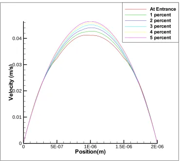
The previous equation is the equation for a fully developed flow in a channel with no slip. The above equation yields a parabolic velocity profile and this result was verified using COMSOL.

After performing several simulations with COMSOL it was determined that the velocity profile became fully developed around 5% of the channel length, which means that a developing profile need not be taken into consideration when performing calculations. A developing profile will not have a parabolic velocity profile while a fully developed flow will have a perfect parabolic velocity profile, proof of this will be shown later. The results

Position(m)

Ve

lo

ci

ty

(m

/s

)

0 5E-07 1E-06 1.5E-06 2E-06

0 0.01 0.02 0.03 0.04

At Entrance 1 percent 2 percent 3 percent 4 percent 5 percent

Figure 4.1 The developing velocity profiles.

Channel Length (m)

P

res

su

re

(P

a)

0 2E-06 4E-06 6E-06 8E-06 1E-05 101280

101290 101300 101310 101320

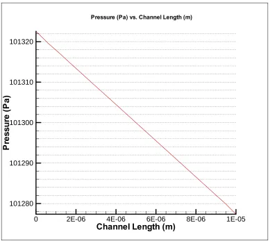
Pressure (Pa) vs. Channel Length (m)

Figure 4.2 Pressure drop across channel length

Figure 4.3 Velocity profiles across the channel length.

The velocity profile plot also indicates that the flow is developed for a majority of the channel. Hence it is safe to assume developing flow while performing our calculations. This assumption is very important as it is required while performing drag force calculations on the particle. It is necessary to know the particle velocity as well as the fluid velocity in order to compute the drag force accurately.

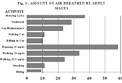
doing some light work. This data was obtained from research conducted by Dr. John R. Holmes titled ‘Measurement of Breathing Rate and Volume in Routinely Performed Activities’ in the California Environmental Protection Agency.[18]

Figure 4.4 Human breathing rates.

Source: http://www.arb.ca.gov/research/resnotes/notes/94-11.htm

The pressure drop was determined using the Hagen Poiseuille equation which was derived in Chapter 3. The following boundary conditions were used to calculate the pressure drop

• Air density: 1.1933×10-5 kg/m3

• Air viscosity : 1.983×10-5 kg ·/ms

Now only 34% of the filter area is holes. So a filter with a 1cm radius would approximately have 34×106 holes with a radius if micron each. Now the mass flow of air will be split equally among all these holes hence the discharge Q will be equal to 7.3529×10-12m3/s. Plugging all the above values in the following equation

4 8 LQ P

r

μ π

Δ =

We get Δ ≈P 3500Pa

This would be the required amount of pressure drop in order to use the filter in a breathing device. The problem with such a high pressure drop is that the filter might not be able to handle it. It has to be determined whether the filter can actually withstand such a high pressure drop.

4.1 The Slip Condition

This model does not take slip into consideration. The slip boundary condition becomes significant when the Knudsen Number lies between 0.01 and 0.1. The Knudsen number is the ratio of the mean free path of the media ( In this case air) and the characteristic length scale.

Or we can say that

Kn

h

λ

=

length scale of the filter is 2 microns. After substituting the values we get Kn as 0.0325. This means that this flow will lie in the slip regime. The effect of the slip boundary condition has to be determined, and also we will have to estimate the error that will be introduced due to the exclusion of this boundary condition. First let us derive the equation including the effect of the slip boundary condition.

We know that 2

2 x

v dP

dx μ y

∂ =

∂ (This equation will be derived in Chapter 4) (4.1.1)

Upon integrating twice with respect to ‘y’ we get 2 1 2 1 2 x dP

v y C y C

dx

μ

= + + (4.1.2)

2 0 s At y U C ⇒ = = And At y=h

2 1 1 2 s s dP

v h C h v

dx

μ

= ⋅ + + (4.1.3)

2 1

1 2

dP

C h h

dx

μ

− = ⋅ (4.1.4)

1 1 2 dP C h dx μ

⇒ = − ⋅ (4.1.5)

Using the constants in Eq. 2.1.2 we get, 2

1 1

2 2

x s

dP dP

v y hy v

dx dx

μ μ

= − + (4.1.6)

2 2

2

x s

h dP y y

v v

dx h h

μ

⎡_{⎛ ⎞ ⎛ ⎞}⎤ ⇒ = _{⎢⎜ ⎟} −_{⎜ ⎟⎥}+

⎝ ⎠ ⎝ ⎠

⎢ ⎥

⎣ ⎦ (4.1.7) Where v_sis the slip velocity denoted by the following equation,

2 ( / ) x s dv v Kn

d y h

σ σ

−

= (4.1.8)

Also from Eq. 2.1.7 2

2 1 ( / ) 2

x

dv h dP y

d y h μ dx h

⎡ ⎤

= _⎢ − _⎥

Using the previous equation in Eq. 4.1.8 we get 2

2 2

1 2

s

h dP y

v Kn

dx h

σ

σ μ

− ⎡ ⎤

= _⎢ − _⎥

⎣ ⎦ (4.1.10)

The constant σ is determined experimentally and generally has a value of 0.85 to 1.0, some experiments in micro-channels conducted by Arkilic et al. yielded values ranging from 0.75 to 0.85. Using the above equation the slip velocity is obtained as 0.019 m/s for a centerline velocity of 0.05m/s [15]. The effect of the slip velocity on the velocity profile is shown in the following figure.

Figure 4.5 The slip and no slip velocity profiles.

considered) compared to the no slip condition (where the particle gets deposited as soon as it touches the wall). This is a small inaccuracy that has not been taken into consideration in this model.

Figure 4.6 Velocity field with no-slip condition

Figure 4.7 Velocity field with slip condition.

Chapter 5

Simple Models

To achieve the kind of modeling described in Chapter 4 first we have to create certain

geometry. This geometry will be representative of a portion of the filter i.e. about 5 channels. Since in this case we are assuming the filter to be isotropic to start with it would be wise to consider modeling only a certain area of the filter. This is because a filter may have say more than one thousand holes in an extremely small area. Therefore meshing and solving this geometry would require a tremendous amount of computing time and power.

The problem we are dealing with is a coupling of two different physics i.e. Electrostatics and Laminar Flow. The solver in COMSOL Multi-physics uses a general version of the Navier Stokes equation to account for variable viscosity, even though we consider only

incompressible flow [19].

[ ( ( ) ]T ( ) u

u u u u p F

t

ρ∂ − ∇ ∇ + ∇η +ρ ∇ + ∇ = ∂

0

u

∇ ⋅ =

To start with, we consider one channel (a channel is considered in the shape of a cylinder) and apply the following boundary conditions.

• One face is considered as inlet and the other face is considered as outlet.

• The inlet and outlet rings of the cylinder are imparted with a uniform line charge of density of 2.64×10-11 C/m

• No slip condition is assumed at the walls.

• Channel radius =1×10-6 m

• Channel length = 1×10-5 m

At the outlet there are two types of boundary conditions that can be specified - • Pressure, no viscous stress

• Pressure

The first boundary condition can admit total control of pressure level at the whole boundary. This condition is also numerically stable. This boundary condition is used when the flow is more or less normal to the face of the channel. If the flow is not normal to the channel face this boundary condition is an over specified one [19]. Since in this case the flow is more or less normal to the channel face this boundary condition is used.

εis the permittivity of the medium, εr is a dimensionless constant known as relative permittivity.εois a constant having a value of 8.854 ×10-12F/m.

E is the electric field intensity required to produce the electric flux density D in a given medium or material of permittivityε. For all linear materials the directions of E and D are the same.

In the previous plot we can see the distribution of pressure inside the channel. As imposed in the boundary condition we can see there is a relatively higher pressure at the inlet and a lower pressure at the outlet.

Figure 5.3 Subdomain plot of the Electric Field

models in COMSOL have been made as close to the actual filter in terms of geometry, charge distribution and material properties.

Figure 5.4 Particle Trace in a Single Channel

This may be done by solving the Langevin Equation [21]

+

D E B

du

m F F F

dt = + (5.1)

D

F =Drag Force acting on the particle = 6πμa K u[ _{p p}−K u_{f f}]

E

F

2 2

0 2 exp( [ ]) ( )

2

[ ]

exp(2 [ ]) 1

p m p m

r h a

g h a

ψ ψ κ ψ ψ πκε ε κ − − + − − B

F

t

π μ ς

Δ

Where, K_pand K_f are the additional hydrodynamic hindrances described by diagonal matrices, u_p is the unperturbed velocity vector for the particle, u_f is the fluid velocity, κ is the inverse Debye length,ε_r is the dielectric constant,ε₀ is the permittivity of free space, h

is the distance of closest approach, ψ_pis the surface potentials of the particle, ψ_mis the surface potential of the membrane, k _B is the Boltzmann constant, Δt is the time step taken

ς is a Gaussian random number with unit mean and zero variance, a is the particle radius,μ is the dynamic viscosity and Tis the temperature

Equation (5.1) is a modified version of Newton’s second law. Newton’s second law states- The rate of change of linear momentum is directly proportional to the net force applied on the object and inversely proportional to its mass.

Mathematically we can say thatF ∝a.

F = ⋅m a

It is known that acceleration ‘a’ is the second derivative of displacement i.e. 2

2 d x a

dt

= or we can say that F m du

dt

= ⋅ (since it is known thatu dx dt = )

Out of these three forces only the Brownian force was successfully modeled. Incorporating the drag force is a little bit harder since the fluid velocity varies parabolically along the channel diameter and that is hard to take into account while solving six sets of differential equations simultaneously. There are six sets since each direction i.e. x y and z will have two sets of equations. The second order equation is broken into two first order equations as shown below.

+ ; x

D E B x

du dx

m F F F u

dt = + dt =

Figure 5.5 Brownian motion of the particle (no initial velocity)

Figure 5.6 With 0.5m/s initial velocity in Y direction

Figure 5.7 With 0.5m/s initial velocity in Z direction

Chapter 6

Multi-channel Model

The multi channel model of the filter gave much better results. Even though solving it took extremely large amounts of time the results obtained were excellent.

Figure 6.1 Multi channel model geometry.

domains is air having a density if 1.165 kg m/ 3. The filter material used was nylon having a density of 1150 kg m/ 3 and having an electrical permittivity of 4. The density of air was taken as 1.165 3

/

kg m and the coefficient of dynamic viscosity was taken as 5

1.9 10× − kg ms/ .

Figure 6.2 Mesh consisting of 41382 elements

Figure 6.3 Electric line charge distributed on filter rings

Figure 6.4 Electric potential rings on filter surface

Figure 6.5 The above figure gives a brief overview of the EFM process.

The above figure shows the holes that were scanned across during the actual EFM measurements.

-5 0 5 10 15 20 25

0 2 4 6 8 10 12

X (μm )

P

h

ase Shi

ft

A

n

gl

e (

D

egr

ee) -10V_-5V

0V 5V 10V

Figure 6.7 EFM measurement results [22]

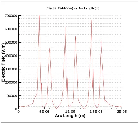
Figure 6.7 show the results from the actual EFM measurements [22]. The plot shows how the phase shift angle varies with the variation in applied bias voltage. The above plot gives a qualitative idea of how the field across the filter will vary. The derivative of the phase shift angle is proportional to the electirc field. A similar simulation was carried out using

Arc Length (m)

El

e

ct

ri

c

F

ie

ld

(V

/m

)

0 5E-06 1E-05 1.5E-05 2E-05

0 100000 200000 300000 400000 500000 600000 700000

Electric Field (V/m) vs. Arc Length (m)

Figure 6.8 Variation of electric field across filter surface

Arc Length (m)

E

le

ct

ric

P

o

te

n

tia

l(

V

)

0 5E-06 1E-05 1.5E-05 2E-05

0 1 2 3 4 5

Electric Potential (V) vs. Arc Length (m)

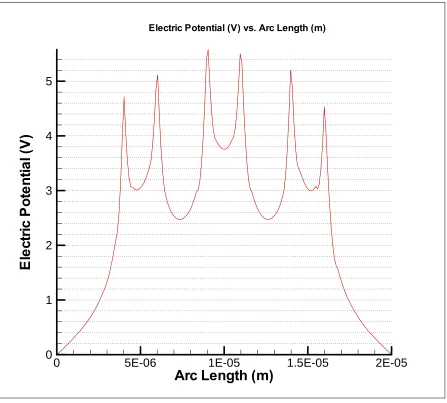
Figure 6.9 Variation of Electric Potential Across Filter Surface

Figure 6.9 shows the variation in electric potential across the filter surface. It can be seen that the peaks represent the rings of charge on the filter surface and the small depressions

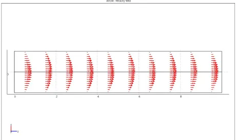
Figure 6.10 Arrow plot of velocity field.

Figure 6.10 shows us the velocity profile of the air flow inside the channel. We can see that the flow becomes fully developed in a very short period of time. As proved for the single channel model it is safe to neglect developing flow since the flow is developed for a major portion of the channel length.

Figure 6.11 Multi-Channel Filter Geometry.

Figure 6.12 Filter with 100 particle traces.

Chapter 7

Determining the Filter Strength

The filter being taken into consideration can have many applications and it has to be

determined whether it will be suitable for them. For example one of the potential applications of this filter would be for breathing purposes. This has been explained in detail in Chapter 4. In that chapter it was derived that the pressure drop required for a breathing application would be around 3500Pa . Now it has to be determined whether a filter with such limited thickness will actually be able to withstand such a high pressure drop. This can be done using any FEA commercial package such as COMSOL Multi-physics.

The experiment will require a filter of a reasonable diameter of about 0.5cm to 1cm. It has to be determined what size and shape will be appropriate. This task is not easy since the length scales involved in this problem are huge. The diameter of the filter is in the range of

0.5~1cm, the thickness of the filter is only 10 micrometers and the hole size is only 1 micrometer. When such a geometry is meshed in COMSOL it takes a huge amount of memory since the mesh will be extremely fine near the holes and near the filter length. This makes the problem nearly impossible to solve. Therefore we have to make certain

approximations before such an analysis is performed. Since the holes are only 1 micrometer in diameter they are the hardest to mesh. Therefore only the filter membrane is modeled without the holes. After this some sort of scaling has to be performed in order to estimate the stresses in the filter with the holes present.

Table 7.1 Boundary Conditions

Young’s Modulus Poissons Ratio Density (Polypropylene)

2 GPa 0.34 0.9g/cc

The following boundary conditions were used.

Sides 1, 2, 5 and 6 are fixed and have zero displacement in all directions. Side 3 has a pressure of 50 Pa spread uniformly.

Side 4 is left as is.

Sides 1, 2, 5 and 6 are the sides (of length 0.5cm) of the square filter and sides 3 and 4 represent the face. The following figure illustrates the filter mesh and geometry.

The geometry is meshed using a tetrahedral mesh. The total number of boundary elements was limited to only around 500. The total number of elements in the mesh was 41837

elements. Figure 7.1 shows the mesh that was used to perform the analysis. Results from the analysis are shown below.

Figure 7.2 Contour Plot Showing Stress Distribution (Max Stress 2.9MPA)

increased four times. Therefore even a 1 cm by 1 cm membrane would be safe under a pressure of 50 Pa.

It is interesting to note that the shape of the filter also determines the amount of stress it can handle. Again an analysis had to be performed to determine what shape would be able to handle a greater amount of stress. The size of the filter is extremely large compared to the size of the holes. Meshing a full size filter with the holes would require an extremely fine mesh and would require a very fast computer with a large amount of memory. To make initial rough estimates with the limited amount of computing power available a membrane was considered without any holes. Two shapes considered were a square and a circle. Since the computation time for a circle was extremely long, smaller dimensions were considered, i.e. both geometries were scaled down while keeping their respective areas the same.

Figure 7.3 shows the mesh used for the square membrane. The number of elements in the mesh is about 18000. The above picture shows the mesh and the geometry of the membrane considered. The membrane has sides of length 0.0018 m.

Figure 7.4 Circular membrane meshed using a tetrahedral mesh.

Figure 7.5 Stress distribution for the circular filter (Max stress 0.32MPa)

Figure 7.6 Stress distribution for a similar size square filter (Max Stress 0.41MPa)

Chapter 8

Experimental setup

In order to verify all the theoretical predictions it is necessary to conduct experiments. The experimental setup involved uses state of the art equipment. It consists of

• Diffusion Dryer/Atomizer

• Electrostatic Classifier

• Condensation Particle Counter

• Transparent Plastic Tubes (4inch diameter)

• Tube Flanges and Mountings

• Polypropylene Filter

• Polystyrene particles

• Digital Pressure Gauge

Diffusion Dryer

The diffusion dryer is a device used to remove water vapor from the particulate flow. The dyer consists of a removable extractor and a desiccant. The removable extractor collects large water droplets while the desiccant removes excess moisture by diffusional capture.

Figure 8.1 Diffusion Dryer

Source www.tsi.com [24]

Since the desiccant never comes in contact with the flow the particle loss is reduced to a minimum and the desiccant can be reused again by heating it to a temperature of 120 degrees Celsius. After leaving the diffusion dryer the particle airstream enters the electrostatic

Electrostatic Classifier

The main function of the electrostatic classifier is to separate out highly mono-disperse aerosols ranging from 2-1000 nm in particle diameter. The particles used in this experiment are polystyrene particles, these may have varying sizes and it is necessary to separate out or classify these particles such that only the required range of particles are released to the filter.

Figure 8.2 Electrostatic classifier

This classifier mainly consists of a Kr 85 Bi-Polar charger, Differential Mobility Analyzer (DMA) and an impactor. The Kr 85 Bi-Polar charger neutralizes the particle charge by exposing the aerosol particles to a high concentration of Bi-Polar ions. This leads to frequent collisions between the particles due to the random thermal nature of the ions. Because of this the particles reach a state of equilibrium where the charge on the particles is known.

The inner cylinder receives the particles and the outer cylinder receives sheath air. Both the streams flow downwards in a laminar flow regime and do not mix. The inner cylinder known as the collector is maintained at a controlled negative voltage while the outer cylinder is grounded electrically. This charge distribution on the cylinders creates an electric field. Now the negatively charged particles are attracted towards the collector i.e. the inner cylinder.

Figure 8.3 Differential mobility analyzer (DMA)

The particles are collected at different portions of the collector based on their electrical mobility. Particles with high mobility are precipitated along the upper portion of the collector and particles with lower mobility are collected at the lower half. Particles with limited

The main function of the impactor is to remove particles that may be larger and carry more than a single charge. It does this by using the principle on inertial impaction. When the stream enters the impactor its velocity is increased by a converging section which is directed towards a flat plate. Upon impacting the plate the streamlines in the flow turn by an angle of 90 degrees. Heavier particles which have more inertia are not able to follow the streamlines. Lighter and smaller particles, which much lesser inertia, continue to follow the streamlines and enter the classifier.

The impactor also functions as a flow meter; this is because the square root of the pressure drop across the impactor is proportional to the flow rate.

Figure 8.4 The impactor.

Figure 8.4 shows the impactor connected to the aerosol inlet of the Classifier.

Condensation particle counter

The condensation particle counter is a water based continuous laminar flow instrument. It helps to determine the particle concentration for particles as small as 5nm. It draws in a sample of air and counts the number of particles and displays the results in terms of the number of particles per cubic centimeter of air. It does this by using a laser and an optical detector. The particles are illuminated by the laser and their size is amplified by using water vapor. It would be hard to detect particles without increasing their size since their diameter is extremely small. The particle stream first enters a region where it is wetted. The stream then passes through a growth section where its temperature is increased to produce and elevated vapor pressure.

Figure 8.5 Condensation particle counter.

continues to condensate on the particles as it moves up the growth tube and the enlarged particles are then detected by the particle counter. The condensation particle counter is connected to the inlet and the outlet of the filter test section. The particle counter counts the number of particles released into the stream before filtration and then also counts the number of particles downstream. This helps in calculating the filtration efficiency [25].

Chapter 9

Results and Conclusions

Figure 9.1 shows the behavior of the particle (weighing 4.3×10-18 Kgs and having a radius of 1×10-7m) as it enters and tries to exit the channel. The particle has a charge of -1e and the filter is positively charged. This leads to an attraction force between the filter and the particle and this helps in further accelerating the particle as it moves through the channel. Since the particle momentum is increased by such a large factor it fails to get captured by the filter. The particle acceleration is shown by the colors in the particle trace.

In the following figure, the particle density is left unchanged and the particle charge is changed from -1e to +1e. 

Figure 9.2 Positively charged particle repelled away from the filter.

Here we can see that the particle does not even get near the filter face and gets repelled by the electric field. It can also be seen that the maximum velocity is also significantly smaller since the particle is not accelerated the way it was in the previous case.

Here is a summary of the boundary conditions used. Table 9.1 Boundary Conditions.

Particle Mass (Kgs)

Particle Radius (m)

Pressure Drop (Pa)

Charge on Particle

Charge on Filter Ring (C/m)

Figure 9.3 Five positively charged particles released at once.

Figure 9.4 Particle charge increased to +3 electrons.

Figure 9.5 Particle charge increased to +7 electrons.

Figure 9.6 Particles with -3electrons charge

Figure 9.7 Particles with no mass and electric charge.

Figure 9.8 Particle oscillating in an inviscid medium

A second multi-channel model was described in Chapter 6; this model was created such that it could accommodate larger particle sizes which would be immune to the effects of

Brownian motion. This model is also capable of handling a large number of particles during a single simulation and was used to determine the variation of filtration efficiency with

increase in particle radius. The results obtained from the simulation are shown below.

Figure 9.9 Variation of filtration capture efficiency with particle radius

consequence, i.e. it also shows that larger particles are not affected by the electric field of the filter, whereas in the first multi channel model the particles were strongly repelled by the filter since the particle mass was much smaller.

9.1 Conclusions

From the results derived from the previous chapters the following conclusions can be drawn. • The governing equations for the flow in the channels are the Navier Stokes Equations

with the Slip Boundary Condition.

• The flow in the filter channels becomes fully developed after roughly 5% of the channel length.

• This filter cannot be used for breathing purposes unless the material is changed from poly-propylene to something that has much higher yield strength.

• The ideal pressure drop for conducting experiments with this filter would be less than 50Pa.

• A circular filter with the same area as a square filter will be able to handle a slightly higher pressure drop.

• The electric field and the drag force play a strong role in capturing particles.

• The filter capture efficiency increases with increase in particle charge.

• Particles having a mass larger than 1×10-15 Kgs are not affected by the electric field of the filter surface.

• The charge concentration on the filter rings is affected by the surrounding rings and hence the rings in the center will have a greater charge compared to the outer rings. • If the filter was used in a vacuum the particles would oscillate in and out of the filter.

9.2 – Future work

• Include the effects of Brownian motion by using the differential equation module in COMSOL Multi-Physics.

• Include the slip boundary condition and determine whether the inclusion of this boundary condition affects the filtration efficiency.

• Include the effects of dendrite formation.

REFERENCES

[1] Lemons, D.S. (2002), “An Introduction to Stochastic Processes in Physics,” The John Hopkins University press.

[2] Uhlenbeck, G.E and L.S.Ornstein (1930): "On the theory of Brownian Motion," Phys.Rev. 36:823–41.

[3] Kim, M. and Zydney, A.L (2003) “Effect of electrostatic, hydrodynamic, and Brownian forces on particle trajectories and sieving in normal flow filtration,” Journal of Colloid and Interface Science.

[4] Kim, M. and Zydney, A.L (2004) “Particle –particle interactions during normal flow filtrations: Model simulations.

[5] Oh, Y.W, Jeon, K. J, A.I, Jung, Y.W, Jung (2002) “A Simulation Study on the Collection of Submicron Particles in a Unipolar Charged Fiber,” Journal of Aerosol Science and

Technology.

[6] Mazé, B. and Pourdeyhimi, B (2008) “Case Studies of Air Filtration at Microscales: Micro- and Nanofiber Media,” Journal of Engineered Fibers and Fabrics.

[7] Gulijk, C.V and Bal, E. (2008) “Experimental evidence of reduced sticking of nanoparticles on a metal grid,” Journal of Aerosol Science and Technology.

[8] Belfort, G. and Nagata, N. (1985) “Fluid Mechanics and Cross-Flow Filtration,” Elsevier Science Publisher.

[9] Bowen W.R. and Sharif A.O. (1997) “Hydrodynamic and Colloidal Interactions effects on the rejection of a particle larger than a pore in microfiltration and ultra-filtration

membranes,” Chemical Engineering Science.

[10] Bowen W.R.et al. (1999) “A Model of the Interaction Between a Charged Particle and a Pore in a charged membrane Surface,” Advances in Colloid Interface Science.

[11] Boskovic et al. (2008) “Filter efficiency as a function of nano-particle velocity and shape,” Journal of Aerosol Science.

[13] Wang.J and Pui D.Y.H (2008) “Filtration of aerosol particles by elliptical fibers: a numerical study,” Springer Science and Business Media.

[14] Zeman L.J. and Zydney A.L. (1996) “Microfiltration and Ultrafltration” Marcel Dekker Inc.

[15] Panton, R (2003), “Incompressible Flow,” John Wiley and Sons Inc.

[16] Kasiraman, G. (2006) “Advanced Fluid Mechanics,” S.R.M University, unpublised. [17] Bansal, R.K. (2006) “Fluid Mechanics and Hydraulic Machines,” Laxmi Publications Pvt. Ltd.

[18] Holmes, J.R. (1994) “Measurement of Breathing Rate and Volume in Routinely Performed Activities,” National Technical Information Service.

[19] FEMLAB 3 user guide (2003) COMSOL Inc.

[20] Cook, R.D. (2001) “Concepts and Applications of Finite Element Analysis,” John Wiley and Sons Inc.

[21] Kim, M. and Zydney, A.L (2003) “Effect of electrostatic, hydrodynamic, and Brownian forces on particle trajectories and sieving in normal flow filtration,” Journal of Colloid and Interface Science.

[22] Zhu, H. (2009) “Modeling Of Flow Containing Nano-particles Through Electro-statically Charged Monolith Filters,” unpublished raw data.

[23] Tensile strength, http://en.wikipedia.org/wiki/Tensile_strength.