Generalized Eigenvalue Problems: Algorithms and Applications.

(1)

ABSTRACT

MIN, EUN JEONG. Generalized Eigenvalue Problems: Algorithms and Applications. (Under the direction of Dr. Hua Zhou.)

Nowadays we encounter massive data from various fields, and there are growing de-mands for efficient methods to transform data into the useful information. Especially, most data from various research areas contain observations of more than two variables, which we call “multivariate data”. Many statistical methods have been developed to extract useful information under the category “multivariate data analysis”. As dimen-sionality of the data gets bigger with the development of technologies, many statisticians are striving to keep pace with this change by proposing updated methods that are appro-priate for those data. There are at least two characteristics of the recent data. One is high dimensionality, the data gets bigger and bigger. In many cases the number of variables is much larger than the sample size. The other one is the complexity. Multi-dimensional array data, known as a tensor, is emerging. The imaging data is the representative one. Only a few statistical methods exist to handle these data. In this dissertation, we study some tools to deal with the data with these characteristics.

In Chapter 2, we suggest a unifying approach for many constrained multivariate anal-ysis methods. It is well known that many multivariate analanal-ysis methods are based on the generalized eigenvalue problem, which can be formulated as an optimization problem. Building on this relationship, we can solve constrained multivariate analysis problem using existing optimization algorithms. We introduced five classes of optimization algo-rithms to solve the constrained generalized eigenvalue problem and tested their effective-ness on some sparsity or nonnegativity constrained statistical problems.

(2)

(3)

(4)

Generalized Eigenvalue Problems: Algorithms and Applications

by Eun Jeong Min

A dissertation submitted to the Graduate Faculty of North Carolina State University

in partial fulfillment of the requirements for the Degree of

Doctor of Philosophy

Statistics

Raleigh, North Carolina 2015

APPROVED BY:

Dr. Brian Reich Dr. Eric Laber

Dr. Yichao Wu Dr. Hua Zhou

(5)

DEDICATION

(6)

BIOGRAPHY

(7)

ACKNOWLEDGEMENTS

I would like to express my sincerest gratitude and appreciation to my advisor Dr. Hua Zhou, for his immense help and concerns about me. His intuitive instructions and generous support was my driving force in the PhD research. It was a tremendous fortune to me that I could watch and learn his profound insight and professionalism for the last three years. Time that I could spent with him in NCSU will be a nourishment for my future academic achievement.

I also would like to express my dearest gratitude and appreciation to my mentor Dr. Hoon Hong and Pauline Hong, for their endless love, help and concerns about me. Their continued concerns were great motive power for me to finish my research. Especially extremely valuable advice from Dr. Hoon Hong will be a spiritual nourishment for the future research.

I am grateful to Drs. Yichao Wu, Brian Reich and Eric Laber for being committee members for my PhD study. Their insight was a great help to my PhD research. I am grateful to Dr. Huixia Judy Wang. For the first two years in NCSU, she was a great guide to my study. Her valuable advice and warm words were great help to me, and the fuel for my study. Also, I thank Dr. Charlie Smith. For almost two years, I got his warm concerns and greetings while I worked as his teaching assistant. Also, I would like to thank Drs. Kim Weems and Howard Bondell for their great help as a graduate program director.

Thanks to my friends in our department. Great time we had together made me happy whenever I feel hard and tired. Their support and encouragement would be a great memory forever. Also thank to friends in my homeland. Their continued contacts and phone calls were a great pleasure during my PhD study.

(8)

Their sacrificial devotion and prays towards me are beyond price; I know I am a beloved person.

(9)

LIST OF TABLES

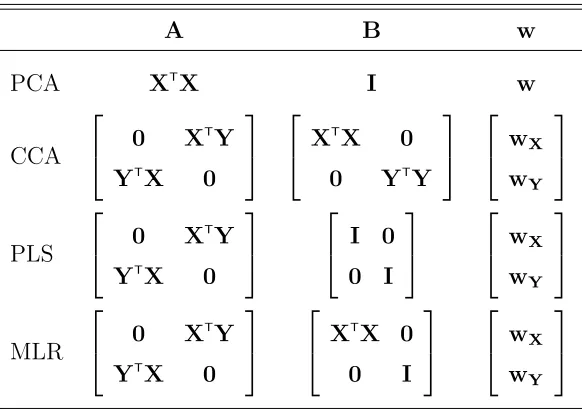
Table 2.1 Reformulation from multivariate problems to GEP. X and Y rep-resent observed datasets from same objects. Since PCA deals only one data set, its expression only contains X. . . 11 Table 2.2 True values of v1 and v2 for generating synthetic data under each

combination of n and p. . . 31 Table 2.3 Boxplots for time consumed and optimized canonical correlation

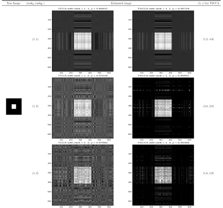
val-ues are displayed for each combination ofn and p. . . 32 Table 3.1 Results of TCCA and TSCCA for the square image. First column

shows a true image, and the rest of 6 images are recovered image by TCCA and TSCCA. Among estimated 6 images, left three images are recovered by TCCA, while right three are by TSCCA. We can observe that rank-1 structured coefficientB catches the signal well enough, higher rank shows overfitting. Also we can observe that image from TSCCA is much clearer than the one from the TCCA. 64 Table 3.2 Results of TCCA and TSCCA for the cross image. First column

shows the true image, and the rest of 6 images are recovered images by TCCA and TSCCA. Among estimated 6 images, left three im-ages are recovered by TCCA, while right three are by TSCCA. We can observe that higher rank structure imposed model shows better signal recovery. Also, we can observe that image from TSCCA is much clearer than the one from the TCCA. . . 65 Table 3.3 Results of TCCA and TSCCA for the circle image. First column

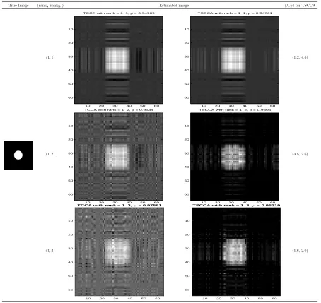
shows the true image, and the rest of 6 images are recovered images by TCCA and TSCCA. Among estimated 6 images, left three im-ages are recovered by TCCA, while right three are by TSCCA. We can observe that higher rank structure imposed model shows better signal recovery. Also, we can observe that image from TSCCA is much clearer than the one from the TCCA. . . 66 Table 3.4 Results of TCCA and TSCCA for the triangle image. First column

(12)

Table 3.5 Results of TCCA and TSCCA for the butterfly image. First column shows the true image, and the rest of 6 images are recovered im-ages by TCCA and TSCCA. Among estimated 6 imim-ages, left three images are recovered by TCCA, while right three are by TSCCA. We can observe that higher rank structure imposed model shows better signal recovery, but we may need higher rank to get better recovery of the triangle signal. Similarly with previous examples, we can observe that image from TSCCA is much clearer than the one from the TCCA. . . 68 Table 3.6 Results of TCCA SEP and TSCCA SEP for the square image. First

column shows a true image, and the rest of 6 images are recovered image by TCCA SEP and TSCCA SEP. Among estimated 6 images, left three images are recovered by TCCA SEP, while right three are by TSCCA SEP. Same as TCCA and TSCCA, we can observe that rank-1 structured coefficientB catches the signal well enough, higher rank shows overfitting. Also, we can observe that image from TSCCA SEP is much clearer than the one from the TCCA SEP. . 70 Table 3.7 Results of TCCA SEP and TSCCA SEP for the cross image. First

column shows a true image, and the rest of 6 images are recovered image by TCCA SEP and TSCCA SEP. Among estimated 6 images, left three images are recovered by TCCA SEP, while right three are by TSCCA SEP. It seems to be enough with rank-2 of the coefficient

B, we can see that the model with rank-3 ofB gives us a overfitted result. Also we can observe that image from TSCCA SEP is much clearer than the one from the TCCA SEP. . . 71 Table 3.8 Results of TCCA SEP and TSCCA SEP for the circle image. First

(13)

Table 3.9 Results of TCCA SEP and TSCCA SEP for the triangle image. First column shows a true image, and the rest of 6 images are re-covered image by TCCA SEP and TSCCA SEP. Among estimated 6 images, left three images are recovered by TCCA SEP, while right three are by TSCCA SEP. We can see that higher ranked mode gives better recovered results. It seems that rank bigger than 3 may required for better recovered image. And we can observe again that image from TSCCA SEP is much clearer than the one from the TCCA SEP. . . 73 Table 3.10 Results of TCCA SEP and TSCCA SEP for the butterfly image.

(14)

LIST OF FIGURES

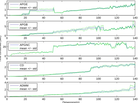
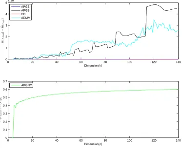
Figure 2.1 Time consumed for getting result from five algorithms. . . 26 Figure 2.2 Plots for comparison between analytical solution and optimal

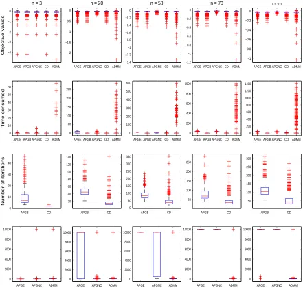
solu-tion from four algorithms. . . 27 Figure 2.3 Boxplot of final optimized value, time consumed (in sec), and total number of

iterations undern= (3,20,50,70,100) for five algorithms. For the number of

iterations, we draw separate boxplots for APGE, APGNC, and ADMM in the

fourth row. . . 29

(15)

Chapter 1 Introduction

1.1 Multivariate Data Analysis

Researchers gather data to answer scientific questions. Most data sets collected in various research areas contain observations of more than two variables. Analysis methods on those multivariate data are highly demanded. To fulfill those demands, statisticians have developed various methodologies to analyze the multivariate data. Multivariate analysis can be thought as a general term to call those methodologies. Multivariate analysis deals with the data that includes simultaneous measurements on more than two variables to get useful information or answers of the scientific inquiries.

(16)

2007; Maletić-Savatić et al., 2008). NMR spectroscopy is the technique that produces a spectrum of a mixture of metabolites in biological samples, resulting high-dimensional data.. For example, the data from Manganas et al. (2007), which is studied in Allen and Maletić-Savatić (2011), has more than 2000 variables from 27 samples. By studying those NMR data, one can determine what kinds of metabolites are contained in the understand biological patterns. Principal Components Analysis (PCA) proposed by Hotelling (1936) is the one of the most widely used dimensional reduction methods. Linear Discriminant Analysis (LDA) and Factor Analysis are also dimension reduction methods. Recently, sparse PCA are also produced to further reduce the dimensionality and aid interpretation Zou et al. (2006); Shen and Huang (2008); Johnstone and Lu (2009).

Another question of interest to researchers is the relationship between several vari-ables. This problem arises in many areas such as social science, chemometrics, biology, and image genetics. For example, Joyner et al. (2009) study relationship between 4 brain size measures and 11 single nucleotide polymorphisms (SNPs). For a high dimensional example, Stein et al. (2010) study the relationship between 31,622 voxels and 448,293 SNPs. Canonical Correlation Analysis proposed by Hotelling (1936) is the one of the popular methods to find the relationship between two sets of variables. Also, grouping similar variables or objects may be the main task of researchers. Logistic Regression, Support Vector Machine (Vapnik and Vapnik, 1998), Discriminant Analysis, and many other clustering or classification methods are proposed for this purpose.

As discussed above, various multivariate methods exist to address different questions. Interestingly several analysis methods such as PCA, CCA, and MLR share same struc-ture. They can be written as the generalized eigenvalue problem. Consider a square matrix

A∈_Rn×n_{. Eigenvalue problem seeks the eigen vector} _x_∈

(17)

satisfies

Ax=λx.

The generalized eigen problem considers two matrices, A ∈ _Rn×n _and _B _∈

Rn×n. The

goal is to find the generalized eigen vector x ∈ _Rn _{and generalized eigen value} _λ _∈

R

that satisfies

Ax=λBx. (1.1)

If the matrixBis the identity matrix, then the generalized eigenvalue problem is reduced to the eigenvalue problem. This means many multivariate methods can be solved by a uni-fying algorithm for the generalized eigenvalue problem such as the QZ algorithm (Golub and van Van Loan, 1996). But in many applications, we want to find solutions that satisfy certain constraints. In this thesis, we investigate a unifying approach for solving constrained multivariate analysis.

(18)

1.2 Tensor Data Analysis

Beyond high dimensionality, data with more than two dimensions have been gathered. Multi-dimensional array, also called a tensor, frequently occurs in many areas such as computer vision, gene expression, engineering, and neuroimaging.

Consider brain imaging data as an example. Electroencephalography (EEG) measures voltage fluctuations of ionic current flows within the neurons of the brain (Niedermeyer and da Silva, 2005). Voltages are recorded by a number of electrodes over a short period at high frequencies. Therefore the data is two dimensional, taking form a matrix. Positron emission tomography (PET) produces a three-dimensional image of functional activities in the body (Valk, 2003). Magnetic resonance images (MRI), which is used to visualize the brain, produces three dimensional data as well. And a neuroimaging procedure us-ing MRI technology, known as functional magnetic resonance images (fMRI), measures brain activity by detecting changes in blood flow (Huettel et al., 2004). This technology produces more than 102 _{MRI images for each subject.}

There have been few methods in literature for handling tensor data, in contrast to the enormous literature on high-dimensional or even ultra high dimensional vector data. One approach is to simply vectorize tensor data and then apply existing methods. But this approach has at least two drawbacks. First, simply vectorizing tensor data yields extremely high dimensional data.. For example, MRI data typically has 128×128×128 voxels and produces more than 2 million variables if we vectorize them. Even worse, fMRI produces 102 _{to 10}3 _{MRI images for each subject, which is almost impossible to analyze}

after vectorization. The second problem is even more serious; vectorization looses the spatial information contained in its own structure.

(19)

struc-ture have been proposed. In the regression context, matrix regression (Zhou and Li, 2014), CP tensor regression that utilizes CP decomposition of tensor (Zhou et al., 2013), Tucker tensor regression that utilizes Tucker tensor decomposition (Li et al., 2013), and tensor partition regression model (TPRM) (Miranda et al., 2015) have been proposed. These methods utilize tensor decompositions to achieve significant reduction in the num-ber of parameters while preserving the array structure of the data. More recently, Li and Zhang (2015) proposed parsimonious tensor response regression for the data containing vector predictive variables and tensor response variables. To achieve the sparsity of the coefficient, they impose existence of irrelevant linear combination of variables instead of irrelevant individual variables.

Following these, several more approaches are proposed. Tensor sliced inverse regres-sion Ding and Cook (2015b) and higher-order sliced inverse regresregres-sions (Ding and Cook, 2015a) deal with tensor dimension reduction problem. Generalized estimating equation for tensor covariates (Zhang et al., 2014), logistic regression for classification of tensor data (Tan et al., 2013), tensor linear support vector machines (Li, 2014) are other pro-posed statistical analysis methods for tensor data.

(20)

1.3 Thesis Organization

The rest of this dissertation is organized in two chapters. In Chapter 2, a unifying approach for finding constrained solution of multivariate analysis is proposed.

There are some proposed algorithms to get a sparse solution of PCA (Zou et al., 2006; Shen and Huang, 2008; Witten et al., 2009; Journ´ee et al., 2010; Allen and Maleti´ c-Savati´c, 2011). And three algorithms proposed by Waaijenborg et al.; Parkhomenko et al.; Witten et al. are most widely known methods to get a sparse solution of CCA. However, these methods are specific to the method and constraint and do not generalized to other constraints rather than sparsity.

We focus on the fact that several multivariate analysis such as PCA and CCA can be represented in one simple form, the generalized eigenvalue problem. And the generalized eigen value problem can be written as an optimization problem of a function, namely the Rayleigh quotient. Based on these relationships, we propose to utilize existing constrained optimization algorithms to solve the problem. Thus, we can freely add constraints to any multivariate problem that can be represented as the generalized eigenvalue problem and solve those problems using one numerical algorithm. In specific, we investigate five numerical optimization algorithms and focus on utilizing those algorithms to constrained multivariate analysis problem. In the simulation study, CCA has been considered with non-negativity and sparsity constraint to show the usefulness of this approach. Numerical studies in Chapter 2 also form the basis of sparse tensor CCA in Chapter 3.

(21)

then introduced.

(22)

Chapter 2 Constrained Generalized Eigenvalue

Problem

2.1 Introduction

(23)

constraints are frequently added for easier interpretation or better reflection of the data structure. Thus the need for the new methods to solve those constrained problems has increased.

For certain methods and constraints, there exist several proposed approaches to han-dle the problem. In the audiovisual source separation problem that uses CCA, the non-negativity constraint is required to interpret the result as energy signals (Wold et al., 2001; Sigg et al., 2007). In this context, algorithm for the non-negative CCA has been proposed (Sigg et al., 2007). On the other hand, sparsity is another representative con-straint required when we deal with the high dimensional data. We seek a sparse solution that helps us to understand and interpret the underlying phenomena better. There are many proposed algorithms for PCA/CCA with sparsity constraint (Zou et al., 2006; Sigg et al., 2007; Sigg and Buhmann, 2008; Waaijenborg et al., 2008; Kim and Cipolla, 2009; Witten et al., 2009; Hardoon and Shawe-Taylor, 2011). In some applications, both non-negativity and sparsity constraints are simultaneously added (Hoyer, 2004; Zass and Shashua, 2006; Allen and Maleti´c-Savati´c, 2011). Besides these, other constraints could be adopted for the better results or applications.

(24)

numeri-cal optimization methods to most constrained multivariate problem instead of developing specific algorithm for specific constrained problem.

For constrained optimization, we consider gradient descent, coordinate descent, and alternating direction method of multipliers. In the simulation study, we compare the performance of these algorithms under two most common constraints: non-negativity and sparsity.

This chapter is structured as follows. In Section 2.2, the problem is formally formu-lated and the relation to multivariate statistical analysis is explained. In Section 2.3, five algorithms for optimization and several algorithms for projection and acceleration are described. In Section 2.4, performance of algorithms is assessed under various situations. Lastly, Section 2.5 contains conclusions.

2.2 Problem

In this section, we provide a precise statement of the problem that will be studied in this chapter. Our approach is based on the relationship between multivariate analysis, the generalized eigenvalue problem, and the optimization problem of the Rayleigh Quotient function. We will describe those relationship and then give a problem statement. First we define the generalized eigenvalue problem.

Problem 1 (Generalized Eigenvalue Problem (GEP)). For two matrices A∈_Rp×q _and

B∈_Rp×q_{, find a vector} _w_∈

Rq and a constant λ∈R that satisfy

Aw =λBw. (2.1)

(25)

A B w

PCA XT

X I w

CCA





0 XT

Y YT X 0     XT X 0

0 YT

Y     wX wY   PLS  

0 XT

Y YT X 0     I 0 0 I     wX wY   MLR  

0 XT

Y YT X 0     XT X 0 0 I     wX wY  

Table 2.1: Reformulation from multivariate problems to GEP. X and Y represent ob-served datasets from same objects. Since PCA deals only one data set, its expression only contains X.

many multivariate statistical methods can be recast as GEP. Above Table 2.1 shows the reformulation from several multivariate analysis problems to GEP.

On the other hand, GEP relates to the function called generalized Rayleigh quotient. The definition of the generalized Rayleigh quotient is as follows.

Definition 1 (Generalized Rayleigh Quotient (GRQ)). Let A∈_Rn×n _{be symmetric and}

B∈_Rn×n _{be symmetric and positive definite. The} _{Generalized Rayleigh Quotient} _R₍_w₎

of A and B is the function in w∈_Rn _{given by}

R(w) = w T_Aw

wT_Bw. (2.2)

(26)

can be reformulated as the constrained optimization problem of the form:

max

w w

T

Aw s.t. wT

Bw= 1.

Using the Lagrangian L(w) with the Lagrange multiplier λ, we can reformulate the problem as follows.

max

w L(w) = maxw w

T

Aw−λwT

Bw.

Taking the first derivative and equating that to zero leads to the GEP (2.1).

Remark 1. The generalized eigenvalue problem (GEP) is closely related to optimizing

the generalized Rayleigh Quotient (GRQ) (2.2). The GEP finds a pair(λ,w)that satisfies the equationAw=λBw. Seeking the smallest (or largest) value ofλand its paired vector

w is equivalent to minimizing (or maximizing) R(w).

Thus, multivariate analysis can be viewed as the optimization of the GRQ with ap-propriately reformulated matrices from observed datasets. This means we can conduct various multivariate analysis via solving a numerical optimization problem. If we con-sider a constrained multivariate analysis, we solve constrained numerical optimization problem.

Problem 2 (Constrained Optimization of Generalized Rayleigh Quotient (COGRQ)).

Consider two matrices A∈_Rn×n _{which is symmetric and} _B _∈

Rn×n which is symmetric

and positive definite. Find w such that

w= argmin

w∈∆

R(w) (2.3)

(27)

Eventually a constrained multivariate analysis is equivalent to calculating two ma-trices A and B from datasets X and Y following the Table 2.1, pluging in them in the Problem 2, and solving the problem. This approach enables us to utilize existing numerical optimization techniques instead of developing a new algorithm for each mul-tivariate analysis problem with a specific constraint. Moreover, we can conduct various multivariate analysis under constraints using one numerical algorithm, which is a great advantage.

In this chapter, we will consider two constraints: non-negativity and sparsity. Defini-tions of constrained spaces are

∆nonneg = {w1+· · ·+wn= 1, w1, . . . , wn≥0}

∆sparse = {w∈Rn :|w1|+· · ·+|wn| ≤γ, w21+· · ·+w 2

n =λ},

whereγ andλare pre-determined penalty parameters. The constraint set ∆nonneg is used when wi are intrinsically non-negative in the underlying application. The condition that

w1+· · ·+wn = 1 is introduced to make the solution identifiable. The constraint set ∆sparse is used when data exhibits high dimensionality so that sparse solution is preferred.

2.3 Algorithms

In this section, we investigate various numerical algorithms for solving constrained optimization of the Generalized Rayleigh Quotient as stated in Problem 2.

(28)

have been proposed to overcome this drawback. However, recent demand for the high dimensional data brings the original gradient descent method back to the attention for its simple and intuitive nature. We will consider three kinds of gradient descent based algorithms: accelerated projected gradient, accelerated proximal gradient, and accelerated projected gradient for nonconvex objective function.

The second one is the coordinate descent algorithm. Coordinate descent algorithm is also the one of the most widely used methods, because it is simple and intuitive.

The third one is the alternating direction method of multipliers (ADMM). ADMM algorithm is based on dual decomposition and augmented Lagrangian method, so it enjoys benefits from both methods. Boyd et al. (2011) demonstrates that ADMM effectively solve many constrained or regularized optimization problems arising from big data.

In summary, we will investigate the following five numerical optimization algorithms: 1. Accelerated Projected Gradient Method with Exact Line Search (APGE)

2. Accelerated Proximal Gradient Method with Backtracking Line Search (APGB) 3. Accelerated Projected Gradient Method for NonConvex Objective Function (APGNC) 4. Coordinate Descent Method (CD)

5. Alternating Direction Method of Multipliers (ADMM)

Each of these algorithms needs projecting a point to a constraint set ∆. We describe projection algorithms for two type of constraints sets:

6. Projection to ∆nonneg 7. Projection to ∆sparse

(29)

2.3.1 Accelerated Projected Gradient Method with Exact Line

Search (APGE)

Let w(t) _{be a current iterate and} _w(t+1) _{be the next iterate. And let} _∇_R₍_w_{) denote}

the gradient of the objective function R(·) at the point w,

∇R(w) = 2

wT_Bw[Aw−R(w)Bw]. (2.4) From the current iterate w(t)_{, gradient descent moves along the direction of} _−∇_R₍_w(t)₎

with stepsize s such that next objective value R(w(t+1)_{) is less than} _R₍_w(t)_).

We can perform the gradient descent with exact line search for the stepsize s, an idea dating back to Hestenes and Karush (1951a,b). Define u = w(t) _and _v ₌ _∇_R₍_w(t)_{) =}

2

w(t)|_Bw(t)[A−R(w

(t)₎_B_]_w(t)_{. We search along the line} _c _7→ _u₊_cv _{emanating from} _u_.

Then the Rayleigh quotient

R(u+cv) = (u+cv)

T_A₍_u₊_cv₎ (u+cv)T_B₍_u₊_cv₎

reduces to a ratio of two quadratics in c. The optimal points are found by setting the derivative

2(v

T_Au₊_cvT_Av₎₍_u₊_cv₎T_B₍_u₊_cv₎₋₍_u₊_cv₎T_A₍_u₊_cv₎₍_vT_Bu₊_cvT_Bv₎ [(u+cv)T_B₍_u₊_cv_)]2

(30)

numerator of this rational function cancel. This leaves a quadratic with coefficients

(vT

Av)(uT

Bv)−(uT

Av)(vT

Bv) (vT

Av)(uT

Bu)−(uT

Au)(vT

Bv) (2.5)

(uT

Av)(uT

Bu)−(uT

Au)(uT

Bv)

for c2_, _c1_{, and} _c0 _{respectively. These coefficients of the powers of} _c _{can be evaluated}

by matrix-vector and inner product operations alone. No matrix-matrix operations are needed. One of the root yields the steepest descent. The unrestricted steepest descent iterate may violate the constraint and has to be projected back to ∆, the constrained space. Projected gradient descent method iterates the two step process (steepest descent and projection to the constrained space) until convergence.

It may suffer from slow convergence but can be readily accelerated by the Nesterov method (Nesterov, 1983, 2004). The Nesterov algorithm accelerates ordinary gradient descent by making extrapolation based on the previous two iterates w(t−1) _and _w(t)_.

Without extrapolation, Nesterov method collapses to a gradient method with the slow non-asymptotic convergence rate ofO(t−1_{) rather than}_O₍_t−2_{). Remarkably, the Nesterov}

method requires essentially the same computational cost per iteration as the unacceler-ated gradient method. The overall algorithm is summarized in Algorithm 1.

2.3.2 Accelerated Proximal Gradient Method with

Backtrack-ing Line Search (APGB)

Consider the following problem,

Problem 3. Consider two matrices A∈_Rn×n _{which is symmetric and} _B_∈

(31)

is symmetric and positive definite. Find w that

minimize R†(w) =R(w) +I∆(w) =

wT_Aw

wT_Bw +I∆(w), (2.6)

where I∆(w) =



 

 

0 w∈∆

∞ w∈/ ∆

and ∆ is the constrained space.

We can easily notice that above problem is same as the Problem 2. R†(w) is non-differentiable due to I∆, making it impossible to apply the gradient descent algorithm.

Proximal gradient method can be considered as a remedy when the objective function is non-differentiable like in (2.6). At each iteration, we minimize the sum ofI∆(w) and the

first order approximation of R(w) at some given point ζ

Q(w,ζ) =R(ζ) +hw−ζ,∇R(ζ)i+ 1

2skw−ζk

2₊_I

∆(w), (2.7)

instead of the sum of I∆(w) and R(w). Through several lines of calculations it can be

shown that the next iterate w(t+1) _{satisfying (2.7) is}

w(t+1) = argmin

w

I∆(w) +

1

2s(t+1)kw−(w (t)₋

s(t+1)∇R(w(t)))k2

. (2.8)

See details in Beck and Teboulle (2009). Expression (2.8) has two parts. Second term in the expression,w(t)₋_s(t+1)_∇_R₍_w(t)_{), is identical with gradient descent procedure. First}

term,I∆ leads us to project the pointw(t)−s(t+1)∇R(w(t)) to the constrained set. Thus

findingw(t+1) satisfying (2.8) is same as conducting gradient descent on R(·) at current iterate and then project that point to the constrained space.

For the stepsize selection, we employ backtracking line search rule. It starts with s(t)

(32)

untilR†(w(t+1)_{) becomes smaller than} _Q₍_w(t+1)_,_w(t)_).

Like APGE, Nesterov acceleration procedure can be applied to accelerate the algo-rithm. The overall algorithm is summarized as Algorithm 2 in Appendix A.

2.3.3 Accelerated Projected Gradient Method for NonConvex

Objective Function (APGNC)

Accelerated projected gradient method for nonconvex objective function (APGNC) is recently proposed by Ghadimi and Lan (2013) to improve the convergence properties of existing gradient descent based methods. APGE and APGB guarantee global convergence and optimal convergence rate only if the objective function is convex. However, if the objective function is not convex, we cannot guarantee that found solution has the global minimum function value. Even worse, the convergence result becomes weakened relative to the convex case. APGNC is devised to overcome the convergence issue. It guarantees the optimal convergence rate even when the problem is nonconvex.

Consider following composite problem for variable w ∈_Rn

minimize Ψ(w) +χ(w)

where



       

       

Ψ(w) = f(w) +h(w)

f ∈ C_L1,1

f(R

n_{), possibly nonconvex}

h∈ C_L1,1

h(R

n_{), possibly convex}

χ is a simple convecx function with bounded domain.

(2.9)

Notice that substituting Ψ(w) as R(w) and χ(w) as I∆(w) and setting h(·) to zero

(33)

procedures,

w(_mdt) ←(1−α(t)₎_w(t−1)

ag +α(t)w(t−1)

w(t) _←_argmin

w{_λ1(t)kw−(w

(t−1)₋_λ(t)_∇_Ψ(_w(t)

md))k2+χ(w)}

wag(t) ←argminw{_β1(t)kw−(w

(t)

md−β(t)∇Ψ(w

(t)

md))k2+χ(w)}.

(2.10)

APGNC has two more variables w(agt), w(_mdt), which are updated iteratively together with

w(t)_{. We can notice that first step for updating} _w(t)

md resembles Nesterov acceleration, since this step extrapolates two points. Like APGB, the second and third steps have an indicator function that projects to the constrained space ∆.

It is important to choose appropriate parameters used in each steps, α, λ and β in APGNC. Authors suggest the following values for the ideal result under the assumption that we know LR, the Lipschitz constant of R(·),

α(t) _{= 2}_/₍_t_{+ 1)}_{, β}(t) _{= 1}_/₂_L

R, λ(t) ∈[β,(1 +α(t)/4)β]. (2.11)

The overall algorithm is summarized as Algorithm 3 in Appendix A.

2.3.4 Coordinate Descent Method (CD)

(34)

the gradient vector (2.4), to zero yields a scalar quadratic function with coefficients

aii

X

j6=i

bijwj

!

−bii

X

j6=i

aijwj

!

,

aii

X

j,j0₆₌_i

bjj0w_jw_j0 !

−bii

X

j,j0₆₌_i

ajj0w_jw_j0 !

, (2.12)

X

j6=i

aijwj

! X

j,j0₆₌_i

bjj0w_jw_j0 !

− X

j6=i

bijwj

! X

j,j0₆₌_i

ajj0w_jw_j0 !

for w_i2, w_i1, and w0_i respectively. Iteration superscripts on wj and wj0 are omitted for

simplicity in the above display. Denote the real roots (if any) of above quadratic equa-tion (2.13) by r1 and r2. Coordinate wi is updated by whichever among the possible candidates gives the smallest objective value R(w). Possible candidates are not the raw value of r1, r2 from the quadratic equation with coefficients (2.12), determined by

con-sidering constrained space and its boundary. For example, if we think non-negativity constraint, there are four possible candidates we need to consider 0, min(max(r1,1),−1),

min(max(r2,1),−1), and 1. After finishing the cycle for updating all coordinates, check

whether w remains in the constraint set and project the point if it places outside of the constraint set. The overall algorithm is summarized as Algorithm 4 in Appendix A.

2.3.5 Alternating Direction Method of Multipliers (ADMM)

ADMM is originally proposed by Gabay and Mercier (1976).

Problem 4 (Problem of ADMM). Given matrices A ∈ _Rp×n_, _B _∈

(35)

c∈_Rp_{. Find} _w_∈

Rn and z∈Rm such that

minimize f(w) +g(z)

subject to Aw+Bz=c.

(2.13)

ADMM algorithm keeps iterating following three steps,

w(t+1) = argmin

w

Lρ(w,z(t),u(t))

z(t+1) = argmin

z

Lρ(w(t+1),z,u(t))

u(t+1) = uk+ρ(A(t+1)+Bz(t+1)−c),

with Lρ(w,z,u) = f(w) +g(z) +uT(Aw+Bz−c) + (ρ/2)kAw+Bz−ck22 and ρ >0.

Problem 2 can be reformulated in the form of the Problem 4 as

minimize R(w) +g(z) = w_wTT_BAw_w+I∆(z)

subject to w−z=0

where

I∆(z) =



 

 

0 z∈∆

∞ z∈/ ∆ ∆ : constrained space.

(2.14)

(36)

w,z and u alternately

w(t+1) ← argmin

w

R(w) + 1

2λkw−z

(t)₊_u(t)_k2 2

(2.15)

z(t+1) ← P∆ w(t+1)+u(t)

(2.16)

u(t+1) ← u(t)+w(t+1)−z(t+1). (2.17)

We can implement the first step (2.15) using any reasonable methods. In this paper we choose APGB introduced in Section 2.3.2. The overall algorithm is summarized as Algorithm 5 in Appendix A.

2.3.6 Projection to

∆

nonneg

Recall that

∆nonneg ={w1+· · ·+wn= 1, w1, . . . , wn ≥0}.

The projection to ∆nonneg can be efficiently carried out by employing Michelot algorithm (Michelot, 1986). Notice that any points in ∆nonneg satisfy two conditions. Michelot al-gorithm alternatively projects the point onto the constrained space, the first constraint is required or the second one is required. Then it removes coordinates satisfying both constraints from the consideration of the next iterate. Michelot algorithm converges in at most n iterations and often much sooner because every iteration reduces the dimension

(37)

2.3.7 Projection to

∆

sparse

Recall that

∆sparse ={w∈Rn :|w1|+· · ·+|wn| ≤γ, w21+· · ·+w 2

n =λ}.

It is trivial that if λ ≥ √2γ, this projection problem is reduced to a projection to l2

ball. Projection to l2 ball can be done by rescaling, as described in Algorithm 10 in the

Appendix A. In a similar way, if λ≤γ, then this projection is reduced to a projection to

l1 ball. Since sign of the projected point should have same sign ofw, we only consider the

absolute value of wi, i= 1, . . . , n. Projection of |w| tol1 ball can be done by Michelot’s

algorithm when γ = 1. If γ is bigger than 1, we can use the projection to the simplex ∆simplex = {w ∈ Rn :

P

wi = γ, wi ≥ 0, i = 1, . . . , n}. This projection algorithm is summarized in Algorithm 8. After projection of |w| we can find the projected point of

w onto l1 ball by restoring their sign. Overall projection to l1 ball is summarized in

Algorithm 9. Lastly, if γ < λ < √2γ, then we can use Dykstra algorithm (Boyle and Dykstra, 1986) summarized in Algorithm 11. This algorithm projects the point to the intersection of convex sets. The overall algorithm is summarized in Algorithm 7.

2.4 Experimental Results

We conduct three simulations with synthetic data under one of two constraints, non-negativity or sparsity. We simulated generic and CCA problem, but note that other multivariate analysis methods that can be transformed to the generalized eigenvalue problem are subject to our algorithms as well.

(38)

practice the projected generalized eigenvector to constrained space corresponding to the smallest generalized eigenvalue supplies a good starting point x(0)_{. In all three}

simula-tions, we use this as a starting point.

First two simulations are conducted under non-negativity constraint and the last one under the sparsity constraint. In each of following subsections, synthetic data description will be introduced, then the results and discussion will be followed.

2.4.1 Non-negativity Constrained Problem for Inputs with Known

Exact Solutions

The goal of the first simulation is to show that our approach is useful even though numerical algorithms generally cannot guarantee to find the global maximum if the ob-jective function is nonconvex. To show the accuracy of algorithms, we will compare the analytic solution and the results from five numerical algorithms introduced in previous section.

For some specific A and B matrices, there is a known analytic solution of Problem 2 with non-negativity constraint. Consider a sequence ofn quantilesτi = _n₊₁i , i= 1, . . . , n.

F andf be the distribution function and density function in order. In the weighted com-posite quantile regression context, the estimator of the model has asymptotic covariance

wT_Aw

wT_BwΣ

−1

X where w is a weight vector for n quantiles, X is covariate, ΣX is covariance

matrix of X, and A, B is

Ai,j = min(τi, τj)−τiτj

Bi,j =f(F−1(τi))f(F−1(τj)).

(2.18)

(39)

distri-bution f and F, there exists a closed form solution w∗ ∈ ∆nonneg. We compared this analytic solution with the results from our five suggested algorithms in terms of run-time and difference between analytic solution and optimized value. For the simulation, we considered n = 3, . . . ,140 which means dimension of A and B, and the standard normal distribution is used as the error distribution. Tolerance value for stopping criteria was 10−4, and maximum iterations limit was set as 10,000. For backtracking line search parameter value η = 0.5 is used, while penalty parameter ρ= 2 is used in ADMM algo-rithm. We have three parameters in APGNC, and the Lipschitz constant LR is required to get an ideal result on APGNC, which is actually unknown. We used a rough guess of

LRaccording to the value of each dimension n. At last, we simulate 50 replicates for each

n so that we calculate mean and standard deviation of time consumed.

Following two figures show the results. Figure 2.1 shows the mean and standard devi-ation of the runtime for each dimension. In this figure, we first notice that all algorithms run fast. For the biggest dimension n = 140, we can get the solution within 30 seconds at maximum. All algorithms except APGNC show fast speed.

Figure 2.2 shows differences between analytic solution and results from each of the five algorithms. Except APGNC, all other four algorithms find exact solution, the difference between the analytic solution and results from algorithms are less than 10−5_{. APGNC}

show less accuracy relative to other four algorithms.

(40)

0 20 40 60 80 100 120 140 0

1

2 APGE

mean +/− std

0 20 40 60 80 100 120 140

0

5 APGB

mean +/− std

0 20 40 60 80 100 120 140

0 20

Time consumed (sec)

APGNC mean +/− std

0 20 40 60 80 100 120 140

0

2 CD

mean +/− std

0 20 40 60 80 100 120 140

0 2 4

Dimension(n) ADMM

mean +/− std

(41)

0 20 40 60 80 100 120 140 0

1 2 3 4 5x 10

−6

Dimension(n)

R

(

xAn

a

l

)

−

¯R( xo

p

t

)

0 20 40 60 80 100 120 140

0 0.1 0.2 0.3 0.4 0.5 0.6 0.7

Dimension(n)

R

(

xAn

a

l

)

−

¯R( xo

p

t

)

APGE APGB CD ADMM

APGNC

(42)

2.4.2 Non-negativity Constrained Problem for Randomly

Gen-erated Inputs

The analytic solution is known for the specific case. We do not have an exact expres-sion of the solution most of the time. To assess the performance of five algorithms, we generated random matrices A∈_Rn×n _and _B_∈

Rn×n

A†_i,j =



 

 

generated from N(0,1) i≥j

A†_j,i otherwise

A=A†+

B_i,j† ∼N(0,1)

B=B†|B†+,

(2.19)

where i,j ∼N(0,0.32). We considered dimensions n = 3, 20, 50, 70, and 100. For each dimension, we simulated 500 replicates and recorded runtime, the numbers of iterations, and final objective values. Same values as the first simulation in Section 2.4.1 has been used for η, maximum iteration limit, tolerance, ρ, and LR.

(43)

APGE APGB APGNC CD ADMM −4 −3 −2 −1 0

n = 3

Objective values

APGE APGB APGNC CD ADMM −2

−1.5 −1 −0.5 0

n = 20

APGE APGB APGNC CD ADMM −1.4 −1.2 −1 −0.8 −0.6 −0.4 −0.2 0

n = 50

APGE APGB APGNC CD ADMM −1.2 −1 −0.8 −0.6 −0.4 −0.2 0

n = 70

APGE APGB APGNC CD ADMM −1 −0.8 −0.6 −0.4 −0.2 0

n = 100

APGE APGB APGNC CD ADMM 0 10 20 30 40 50 60 Time consumed

APGE APGB APGNC CD ADMM 0 50 100 150 200 250

APGE APGB APGNC CD ADMM 0 100 200 300 400 500 600

APGE APGB APGNC CD ADMM 0 200 400 600 800 1000

APGE APGB APGNC CD ADMM 0 200 400 600 800 1000 1200 1400 APGB CD 0 10 20 30 40

Number of iterations

APGB CD 20 40 60 80 100 120 140 APGB CD 0 50 100 150 200 250 300 350 APGB CD 50 100 150 200 250 APGB CD 50 100 150 200 250 300

APGE APGNC ADMM 0 2000 4000 6000 8000 10000

Number of iterations

APGE APGNC ADMM 0 2000 4000 6000 8000 10000

Figure 2.3: Boxplot of final optimized value, time consumed (in sec), and total number of iterations undern= (3,20,50,70,100) for five algorithms. For the number of iterations, we draw separate boxplots

(44)

2.4.3 Sparsity Constrained Problem for Randomly Generated

CCA Inputs

In the third simulation, we compare four algorithms, APGE, APGB, ADMM and CD for solving the sparsity constrained CCA problem. Assume that we have data matrices

X and Y. Then our problem is

minimize −wT_Aw

wT_Bw subject to



 

 

kαk1 ≤γ1, kβk1 ≤γ2

kαk2 ≤1, kβk2 ≤1

where w = (αT_,_βT

)T_, _α _{is the canonical coefficient for} _X_, _β _{is the canonical coefficient} forY,γ1, γ2 are pre-specified penalty parameters, and A,Bare matrices calculated from

X,Y as described in the Table 2.1. Note that we put a negative sign in front of the objective function, since the goal of the CCA is finding a pair of canonical vectors that maximizes the canonical correlation. We can find a pair of sparse canonical coefficients (α∗,β∗) that maximizes the canonical correlation Corr(αT

X,βT

Y). We first generated the data X∈_Rn×p _and _Y _∈

Rn×q,

X=uvT

1+1, Y=uvT2+2, (2.20)

ui ∼N(0,0.52), 1,i,j ∼N(0,0.32), 2,i,k ∼N(0,0.32),

i= 1, . . . , n, j = 1, . . . , p, k = 1, . . . , q.

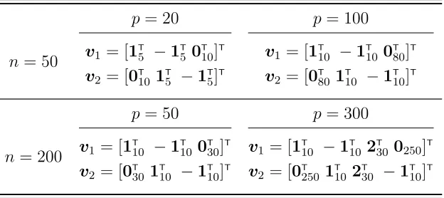
Sparse vectors v1 and v2 in equation (2.20) used under each combination are presented

(45)

combination ofnandpwith 200 repetitions. Parameter values forη, maximum number of

p= 20 p= 100

n= 50 v1 = [1 T

5 −1

T

5 0

T

10]

T _v

1 = [1T10 −1

T

100

T

80]

T

v2 = [0T101

T

5 −1

T

5]

T _v

2 = [0T80 1

T

10 −1

T

10]

T

p= 50 p= 300

n= 200 v1 = [1 T

10 −1

T

10 0

T

30]

T _v

1 = [1T10 −1

T

10 2

T

300250]T v2 = [0T301

T

10 −1

T

10]

T _v

2 = [0T250 1

T

102

T

30 −1

T

10]

T

Table 2.2: True values ofv1 andv2for generating synthetic data under each combination

of n and p.

iterations, tolerance, andρwere set to the same values in other simulations. And we need two more, sparsity parameters γ1 and γ2 that impose sparsity onα and β respectively.

We set same value for both γ1 and γ2, (1, 2.5, 4, 5) has been used for each combination

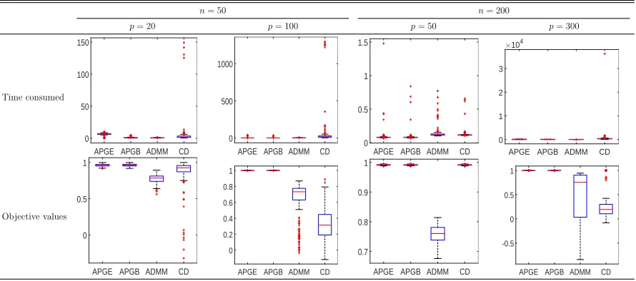
of n and p. Simulation results are summarized as boxplots in the Table 2.3. We can make several observations from results in the Table 2.3. First, APGE and APGB find coefficient sets that result in high objective values. Their results distributed near 1, which means the optimized canonical coefficients give us a high canonical correlation. Moreover, both algorithms do not take much time relative to the other two methods. Especially, APGB shows the fastest speed with good objective values. CD algorithm shows good performance only if number of parameters is less than the sample size. Though it takes more time relative to APGE and APGB, still it gives us good objective values when

(46)

n= 50 n= 200

p= 20 p= 100 p= 50 p= 300

Time consumed

APGE APGB ADMM CD 0

50 100 150

APGE APGB ADMM CD 0

500 1000

APGE APGB ADMM CD 0

0.5 1 1.5

APGE APGB ADMM CD

×104

0 1 2 3

Objective values

APGE APGB ADMM CD 0

0.5 1

APGE APGB ADMM CD

0 0.2 0.4 0.6 0.8 1

APGE APGB ADMM CD 0.7

0.8 0.9 1

APGE APGB ADMM CD

-0.5 0 0.5 1

Table 2.3: Boxplots for time consumed and optimized canonical correlation values are displayed for each combination of n and p.

for moderate accuracy. In this context the results of ADMM can be understood since it takes short time while its final objective values are low in general. Thus there is a possibility that we can get a better result using ADMM, since we only considered one value for the parameter ρ.

2.5 Discussion

(47)

We employ five numerical algorithms some of which are well known.

The great advantages of this approach are three points. First, we can easily add conditions we want, not only the sparsity but any other condition like non-negativity as we saw in Section 2.4. Second, we can employ well established numerical algorithms instead of developing a new algorithm specific to a certain analysis with a certain constraint. Third, we can conduct several analysis stated above by implementing one algorithm.

There are limitations on this approach too. Rayleigh quotient which is the objec-tive function of this approach is nonconvex function This allows guarantee only for the local convergence. Thus, multiple starting points including our suggested one are rec-ommended. Also employed numerical algorithm may require other parameters such as tunning parameters for convergence. For example, ACNPG algorithm in this chapter has two parametersβandλwhich is decided based on the unknown value, Lipschitz constant

(48)

Chapter 3 Tensor Canonical Correlation

Analysis

3.1 Introduction

Canonical Correlation Analysis (CCA), first proposed by Hotelling (1936), is one of the most widely used multivariate statistical analysis techniques to study the relationship between two multivariate data sets. CCA tries to find a set of coefficients such that the correlation between the linear combinations of each data set is maximal. Demands for the analysis of high dimensional data has increased tremendously due to advancement of technology. For example, the relationship between gene networks and DNA-markers is important for understanding complex diseases such as human cancers (Waaijenborg et al., 2008). High dimensionality of gene expression data causes trouble to apply CCA. Traditional CCA does not work any more when the number of variables is far bigger than sample size since sample covariance matrices become singular.

(49)

inter-pretation despite the huge dimension of input data (Waaijenborg et al., 2008; Parkhomenko et al., 2009; Witten et al., 2009; Lykou and Whittaker, 2010). They adopt various regular-ization methods to shrink the coefficients and conduct variable selection simultaneously. In Chalise and Fridley (2012), several sparse CCA methods are compared to see their difference and performance.

High dimensional data may have huge number of variables but it is still a vector-valued data which can be treated via existing methods. But now we face multi-dimensional array data, also known as a “tensor” data, which is more than just high dimensional. Imaging data is the representative one. Take anatomical magnetic resonance images (MRI, 3D array), and functional magnetic resonance images (fMRI, 4D array) as an example. They possess a multi-dimensional structure. MRI data typically has 2,095,152 = 128×128×128 observations for one subject. Even more, fMRI typically consists of more than 102 _MRI

images for each subjects.

The first approach that we can try is vectorizing array and applying existing sparse CCA methods. This approach has at least two issues. First is the number of parameters. For example, vectorizing MRI data produces more than two million variables. The second is that it ignores the structure of the data, which may cause loss of spatial information. In this chapter, we propose a new CCA approach that can deal with the tensor data (TCCA). To accomplish this, we utilize the tensor decomposition that significantly downsizes model complexity. Moreover, we extend our tensor CCA to tensor sparse CCA (TSCCA), which gives us a sparse solution. We will use the numerical methods developed in Chapter 2 to solve TSCCA.

(50)

will develop our proposed models. Efficient algorithms to estimate parameters in those model and discussion about identifiability issue will be followed. In Section 3.5, several numerical simulation results will be described. Section 3.6 concludes this chapter with discussion of some possible future extensions.

3.2 Literature Review

In this section, we summarized two SCCA methods. Sparse CCA proposed by Witten et al. (2009) is the first one that we will review in this section. Based on Witten et al. (2009), adjusted method has been proposed by Chi et al. (2013), which we will review next.

3.2.1 PMD (Witten et al., 2009)

Penalized Matrix Decomposition (PMD) method has been proposed by Witten et al. (2009). PMD approximates a matrix X by ˆX = PK

k=1dkukvk where dk,uk and vk

minimize the Frobenious norm of X − Xˆ subject to constraints on uk and vk. As a result, we do a regularized version of singular value decomposition. The penalized matrix decomposition problem for K = 1 case can be summarized as follows.

Problem 5. Let X ∈_Rn×p _{be a real valued matrix with rank} _r_≤_min_{_{n, p}_}_{. Find}_d _and

vectors u,v that

minimized,u,v

1

2kX−duv T

k2_F

subject to kuk2

2 = 1, kvk 2

2 = 1, P1(u)≤c1, P2(v)≤c2, d≥0

(51)

They showed that the optimal u and v also solves the following problem.

Problem 6 (rank-1 PMD). Let X ∈ _Rn×p _{be a real valued matrix with rank} _r _≤

min{n, p}. Find vectors u,v that

maximizeu,v uTXv

subject to kuk2

2 = 1, kvk 2

2 = 1, P1(u)≤c1, P2(v)≤c2,

where P1 and P2 are convex penalty functions, and c1 andc2 are constants. The value of

d solving the Problem 5 is uT_Xv_.

Witten et al. (2009) also proposed an algorithm to solve above Problem 6.

It is possible to apply this PMD method for estimating sparse canonical coefficients of two datasets on CCA. Let X ∈_Rn×p _and _Y _∈

Rn×q be data matrices collected on n

subjects. Original CCA proposed by Hotelling (1936) looks for two coefficient vectors u

and v that maximizes Corr(Xu,Y v), the correlation between two linear combination of each datasets. That problem can be written as

maximizeu,v uTXTY v subject touTXTXu≤1, ,vTYTY v≤1 (3.1)

If we assume that covariance matrices of X and Y are identity and add l1 penalty on u

and v, then the problem becomes the following one.

Problem 7 (SCCA (Witten et al., 2009)).

maximizeu,v uTXTY v

subject to uT

u≤1, vT

(52)

which can be solved using PMD algorithm.

3.2.2 Sparse Canonical Correlation Analysis (Chi et al., 2013)

Above proposed SCCA by Witten et al. (2009) can be improved if we relax the as-sumption on covariance matrices. Chi et al. (2013) proposed adjusted version of the method of Witten et al. (2009), which relaxes the identity covariance matrices assump-tion. They started on following basic SCCA model, which is slightly different from the model of Witten et al. (2009).

Problem 8 (SCCA). Let X ∈ _Rn×p _and _Y _∈

Rn×q be data matrices gathered from n

subjects. Find vectors u and v that

maximize uT

XT

Yv−λkuk1−γkvk1

subject to kuk2 ≤1, kvk2 ≤1.

The minor difference with the Problem 7 is that sparsity penalties are added instead of sparsity constraints. If we consider v fixed, it is a convex problem in terms of u and vice versa. Thus we can solve Problem 8 by block relaxation method. The update u∗ for

u is given by

ˆ

u= argmin

u

1 2kY

T

Xv−uk2

2+λkuk1

u∗ =



 

 

ˆ

u/kuk2 ifkuk2 ≥0

0 o.w

(3.2)

Same procedure applies to update ofv.

(53)

(2013) suggested to use adjusted covariance estimates, the problem statement is as fol-lowing.

Problem 9 (SCCA(Chi et al., 2013)). Let X ∈ _Rn×p _and _Y _∈

Rn×q be data matrices

collected on n subjects. Find vectors u and v that

maximize uT

XT

Yv−λkuk1−γkvk1

subject to uT

Σxu≤1, vTΣyv≤1,

where λ and γ are given constants, Σx and Σy are estimated covariance matrices of X

and Y.

Possible issue is that the sample covariance matrices become singular when the num-ber of variables is bigger than sample size. Thus for better performance of the solution of Problem 9, we need good estimators of covariance matrices Σx and Σy. There are many proposed methods to adjust sample covariance matrix (Ledoit and Wolf, 2004; Ledoit et al., 2012; Chi and Lange, 2014). With the adjusted covariance estimates ˜Σx and ˜Σy, we can solve the above problem via iterative algorithm similar to PMD. With fixed v,

u∗, the update of u, is given as follows.

ˆ

u= argmin

u

1 2kΣ˜

−1/2

x X

T

Yv−Σ˜1_x/2uk2

2 +λkuk1,

u∗ =



 

 

ˆ

u

kΣ˜

1/2

x uˆk2

if kΣ˜xuk2 >0

0 o.w.

(3.3)

(54)

3.3 Notation and Basic Operations of Array

Before developing models, we review basic notations and operations of multidimen-sional arrays in this section. More notations and operations of a tensor including all introduced in this section can be found in Kolda and Bader (2009).

We call the dimension of the tensor the mode, also known as the order. For example, the mode/order of a tensorX ∈_Rp1×p2×···pD _is_D_{. For mode-3 tensor}_X_,_x

ijk indicates the (i, j, k)-th element of X. Fibers of tensor X denote vectors made by fixing every indices except one. This term can be thought as an extension of matrix rows or columns to the tensor. For example, if we fix the second and third indices of a tensor X ∈ _Rp1×p2×p3

except the first, we get p2 ×p3 fibers, which is also called column fibers. In the same

manner, we can get p1×p3 number of row fibers and p1×p2 fibers when we fix the third

index, which is called tube fibers.

Next, we introduce a operator that has a vector input and a tensor output. We define an outer productb1◦ · · · ◦bD of D vectorsbd∈Rpd. The result of this outer product is p1× · · · ×pD tensor of which entries are calculated as (a1 ◦ · · · ◦aD)i1,...,iD =

QD

d=1adid.

Next, we introduce three matrix products that are used in this chapter. First, we denote the Kronecker productof two matrices A∈_Rm×n _and _B _∈

Rp×q as

A⊗B=



       

a11B a12B . . . a1nB

a21B a22B . . . a2nB ..

. ... . .. ...

am1B am2B . . . amnB



       

(55)

Whenn =q, the Khatri-Raoproduct of two matricesA∈_Rm×n _and_B _∈

Rp×n, denoted

as A∗B, is defined as follows.

A∗B= [ _a₁_⊗_b₁ _a₂_⊗_b₂ _{· · ·} _a_n_⊗_b_n ].

The resulted matrix has dimensionmp×n. IfAandBare vectors, then theirKhatri-Rao product is identical withKronecker product.

If A and B have same size, i.e., if m = p and n = q, then the Hadamard product is defined by,

AB=

     

a11b11 . . . a1nb1n ..

. . .. ...

am1bm1 . . . amnbmn

      ,

which is the elementwise product. Hadamard product commutes, so we will useiAi to denote

A1 · · · AD =Aπ(1) · · · Aπ(D),

where π is any permutation.

We also introduce several basic operators of tensor that transform a tensor into vector or matrix. The vec operator stacks column fibers of a tensor. Consider a tensor X ∈

R2×2×2 as follows,

X··1 =

   1 3 2 4  

, X··2 =    5 7 6 8   .

Then column fibers of X are

(56)

Thus by stacking above four vectors we can get vecX = [1 2 3 4 5 6 7 8]T_{. One more} operator that we will use constantly ismatricization, which is also known asunfoldingor

flattening. This operator makes a tensor into a matrix by restructuring. When we reshape a tensor, reshaping order matters since we get different matrices by different orders. We specifically callmode-n matricization if we take mode-nfibers as columns and we denote

X(n). Consider the toy example above, 2×2×2 tensorX.Mode-1fibers ofX are column

fibers listed above, thus mode-1 matricizationX(1) is defined as

X(1) =



 

1 3 5 7 2 4 6 8



 .

Likewise, we can find X(2) and X(3)

X(2) =



 

1 2 5 6 3 4 7 8





, X(3) = 

 

1 2 3 4 5 6 7 8



 .

For two tensorsA and X with same dimension and mode, we define inner product of them hA,X i as a sum of elementwise product, hA,X i =P

i1,...,iDai1,...,iDxi1,...,iD.

Lastly, we introduce several identities that are useful in the rest of this chapter.

(57)

dimen-sions,

vec (uvT

) = v⊗u

vec (ABC) = (CT_⊗

A)vecB

(A⊗B)T

= AT_⊗

BT

(A⊗B)(C⊗D) = (AC)⊗(BD) (A⊗B)(C∗D) = (AC)∗(BD).

Proof is given in Appendix B.1.

3.4 Model

In this section, we will develop the model for canonical correlation analysis of two tensor data sets that enjoys a significant reduction on the number of parameters while the spatial information is still preserved. To achieve this goal, we adopt a tensor decompo-sition, which enables us to reconstruct a tensor with fewer parameters than the number of all elements of a tensor. The model that vectorizes data requires huge number of pa-rameters to be estimated which can be a big problem itself. For example if we consider vectorizing the two data which have 100×100×100 dimension each, we have 2×106 parameters to estimates. Instead of the vectorization, we impose a certain structure on two coefficient tensors so that we can deal with a problem with less number of parame-ters. Furthermore, we impose a certain structure on the covariance matrices of X and Y

so that we can handle the covariance matrices much easier.

(58)

on two coefficient tensors. Based on this, we will extend the scope so that we can get a sparse solution from the problem, namely tensor sparse CCA (TSCCA). In the Sec-tion 3.4.3, we will develop a more parsimonious model based on TCCA by imposing so called separable covariance structure on the covariance matrices of two data sets (TCCA -SEP). TSCCA SEP, a sparse version of the TCCA SEP, will follows. Identifiability issue caused by CP decomposition will be treated in Section 3.4.4.

3.4.1 Tensor Decomposition

First, we introduce a key concept of our proposed models, the CANDECOP/PARAFAC (CP) decomposition of a tensor.

Definition 2. A tensor X ∈_Rp1×···×pD _{admits a rank-R CANDECOP/PARAFAC (CP)}

decomposition if

X = R

X

r=1

x(₁r)◦ · · · ◦x(_Dr), (3.4)

where x(_dr) ∈ _Rpd_, _d _{= 1}_{, . . . , D}_, _r _{= 1}_{, . . . , R} _{are all column vectors and} X _{cannot be}

written as the sum of outer products with the rank lower than R.

This relationship can be also represented as X =

r

X(1), . . . ,X(D) z

, where X(d) = [x(1)_d , . . . ,x_d(R)] ∈ _Rpd×R _{following the notation introduced in Kolda (2006); Kolda and}

(59)

Lemma 2. If a tensor X ∈_Rp1×···×pD _{admits a rank-R CP decomposition} _(3.4)_{, then}

vecX = (X(D)∗ · · · ∗X(1))1R

X(d) =X(d)(X(D)∗ · · · ∗X(d+1)∗X(d

−1)_{∗ · · · ∗}

X(1))T

vecX(d) = [(X(D)∗ · · · ∗X(d+1)∗X(d−1)∗ · · · ∗X(1))⊗Ipd)]vecX

(d)_.

For the proof of first two equalities, see Zhou et al. (2013). The last one comes from the second equality of Lemma 1. This Lemma 2 enables us to reformulate rank-R decom-position of the tensor to the mode-d matricization or vectorization of the tensor (Zhou et al., 2013).

3.4.2 Tensor Canonical Correlation Analysis

Consider a pair of random variables (X,Y), whereX ∈ _RI1×···×Idx _andY ∈_RJ1×···×Jdy_.

The goal of the CCA is to find the coefficient tensors A ∈_RI1×···×Idx _andB ∈_RJ1×···×Jdy_,

which maximize the correlation between each linear combination ofX and Y as follows.

Corr(hX,Ai,hY,Bi) = _p Cov(hX,Ai,hY,Bi)

Var(hX,Ai)Var(hY,Bi)

= _p Cov(hvecX,vecAi,hvecY,vecBi) Var(hvecX,vecAi)Var(hvecY,vecBi)

= (vecA)

T_Cov(vec_X_,_vec_Y_)vec_B

p

(vecA)T_Var(vec_X_)vec_A_(vec_B₎T_Var(vec_Y_)vec_B

= (vecA)

T

ΣvecX,vecB(vecB)

p

(vecA)T_Σ

vecX(vecA)(vecB)TΣvecY(vecB)

,

Generalized Eigenvalue Problems: Algorithms and Applications.

ABSTRACT

DEDICATION

BIOGRAPHY

ACKNOWLEDGEMENTS

TABLE OF CONTENTS

LIST OF TABLES

LIST OF FIGURES

Chapter 1

Introduction

1.1

Multivariate Data Analysis

1.2

Tensor Data Analysis

1.3

Thesis Organization

Chapter 2

Constrained Generalized Eigenvalue

Problem

2.1

Introduction

2.2

Problem

2.3

Algorithms

2.3.1

Accelerated Projected Gradient Method with Exact Line

Search (APGE)

2.3.2

Accelerated Proximal Gradient Method with

Backtrack-ing Line Search (APGB)

2.3.3

Accelerated Projected Gradient Method for NonConvex

Objective Function (APGNC)

2.3.4

Coordinate Descent Method (CD)

2.3.5

Alternating Direction Method of Multipliers (ADMM)

2.3.6

Projection to

∆

2.3.7

Projection to

∆

2.4

Experimental Results

2.4.1

Non-negativity Constrained Problem for Inputs with Known

Exact Solutions

2.4.2

Non-negativity Constrained Problem for Randomly

Gen-erated Inputs

2.4.3

Sparsity Constrained Problem for Randomly Generated

CCA Inputs

2.5

Discussion

Chapter 3

Tensor Canonical Correlation

Analysis

3.1

Introduction

3.2

Literature Review

3.2.1

PMD (Witten et al., 2009)

3.2.2

Sparse Canonical Correlation Analysis (Chi et al., 2013)

3.3

Notation and Basic Operations of Array

3.4

Model

3.4.1

Tensor Decomposition

3.4.2

Tensor Canonical Correlation Analysis