Low-Order Modeling of Upstream Flow Disturbances on Wing Aerodynamic Performance.

ABSTRACT

NAGULAKONDA VENKATA, KULA SEKHAR. Low-Order Modeling of Upstream Flow Disturbances on Wing Aerodynamic Performance. (Under the direction of Ashok Gopalarathnam.)

©Copyright 2016 by Kula Sekhar Nagulakonda Venkata

Low-Order Modeling of Upstream Flow Disturbances on Wing Aerodynamic Performance

by

Kula Sekhar Nagulakonda Venkata

A thesis submitted to the Graduate Faculty of North Carolina State University

in partial fulfillment of the requirements for the Degree of

Master of Science

Aerospace Engineering

Raleigh, North Carolina

2016

APPROVED BY:

Venkateswaran Narayanaswamy Kenneth Granlund

DEDICATION

BIOGRAPHY

ACKNOWLEDGEMENTS

TABLE OF CONTENTS

LIST OF FIGURES . . . vi

Chapter 1 Introduction . . . 1

1.1 Introduction to formation flight . . . 1

1.1.1 Wing tip vortices . . . 1

1.1.2 Importance of formation flight and vortex impingement . . . 2

1.1.3 Background for vortex impingement . . . 3

1.1.4 Motivation . . . 3

1.2 Introduction to propeller-slipstream/wing interaction . . . 3

1.2.1 Propeller-slipstream description . . . 4

1.2.2 Importance of studying propeller-slipstream/wing interaction . . . 4

1.2.3 Background for propeller-slipstream/wing interaction . . . 7

1.2.4 Motivation . . . 8

1.3 Outline of the thesis . . . 8

Chapter 2 Low-order modeling of wing with upstream flow disturbances . . . 9

2.1 Weissinger's method . . . 9

2.2 Modification to Weissinger's method to handle vortex impingement on a wing . . 13

2.3 Modification of Weissinger's method for handling the propeller-slipstream impingement on a wing . . . 15

Chapter 3 Results and comparisons . . . 18

3.1 Streamwise-oriented vortex impingement . . . 18

3.1.1 CFD results from literature . . . 18

3.2 Propeller-slipstream impingement on a wing . . . 25

3.2.1 Results from Experiments . . . 25

Chapter 4 Conclusions. . . 47

4.1 Conclusions . . . 47

4.2 Future work . . . 48

LIST OF FIGURES

Figure 1.1 Birds flying in a “V” formation. . . 2

Figure 1.2 Comparison of propulsive efficiency of turboprops and turbofans vs. cruise Mach number. . . 5

Figure 1.3 Google’s Makani tethered wind turbine. . . 6

Figure 1.4 NASA's multipropeller aircraft. . . 6

Figure 2.1 Weissinger’s discretization on a swept wing. . . 10

Figure 2.2 Flow chart for streamwise-oriented vortex impingement on a wing . . . 14

Figure 2.3 Flow chart for handling propeller-slipstream impingement on a wing . . . 17

Figure 3.1 The (i) top view and (ii) side view of the CFD simulation setup from the reference paper [14]. . . 19

Figure 3.2 Comparison of sectional lift coefficient for (1)Baseline, (2)Tip-impingement of vortex and (3)Inboard impingement of vortex cases from CFD data [14] . . 20

Figure 3.3 Comparison of sectional lift coefficient for (1) Baseline, (2) Tip-impingement of vortex and (3) Inboard impingement of vortex cases from low-order method 21 Figure 3.4 Comparison of sectional lift coefficient for (1) Baseline, (2) Tip impingement of vortex and (3) Inboard impingement of vortex cases from CFD data and low-order model results . . . 22

Figure 3.5 Comparison of change in sectional lift coefficient for tip impingement of vor-tex from low-order model and CFD data . . . 23

Figure 3.6 Comparison of change in sectional lift coefficient for inboard impingement of vortex from low-order model and CFD data . . . 24

Figure 3.7 Comparison of change in sectional lift coefficient for inboard and tip impinge-ment of vortex from both the low-order model and CFD data. . . 25

Figure 3.8 Experimental setup showing the wing with circular end plates behind a pro-peller in a wind tunnel. . . 26

Figure 3.9 Case 1A: Comparison of sectional wing lift coefficients for AoA of 4 degrees, 8 degrees, and 12 degrees from low-order model and experimental data from [22] with no jet impingement . . . 28

Figure 3.10 Case 1A: Comparison of total wing lift coefficients for AoA of 0 degrees to 12 degrees from low-order model and experimental data from [22] with no jet impingement . . . 28

Figure 3.11 Case 1B: Comparison of sectional wing lift coefficients for AoA of 4 degrees, 8 degrees, and 12 degrees from low-order model and experimental data from [22] with 18% jet impingement . . . 29

Figure 3.12 Case 1B: Comparison of total wing lift coefficients for AoA of 0 degrees to 12 degrees from low-order model and experimental data from [22] with 18% jet impingement . . . 30

Figure 3.14 Case 1C: Comparison of total wing lift coefficients for AoA of 0 degrees to 12 degrees from low-order model and experimental data from [22] with 36% jet impingement . . . 32 Figure 3.15 Case study 1: Comparison of total wing lift coefficients for AoA of 0 degrees

to 12 degrees from low-order model and experimental data from [22] with no jet impingement, 18% jet impingement, and 36% jet impingement . . . 33 Figure 3.16 Sketch of experimental setup with the fuselage half-model. . . 34 Figure 3.17 Case 2A: Comparison of total wing lift coefficient results from low-order

methods to the experimental data atCTs = 0.6 . . . 36

Figure 3.18 Case 2B: Comparison of total wing lift coefficient results from low-order methods to the experimental dataCTs = 0.93. . . 36

Figure 3.19 Experimental setup of the propeller and wing inside the subsonic wind tunnel. 37 Figure 3.20 Case 3A: Comparison of sectional lift coefficients from low-order method and

experimental data for an AoA of 6.5 degrees at a freestream dynamic pressure of 1.55 in of EG . . . 39 Figure 3.21 Case 3A: Comparison of sectional lift coefficients from low-order method

and experimental data for an AoA of 11.5 degrees at a freestream dynamic pressure of 1.55 in of EG . . . 40 Figure 3.22 Case 3B: Comparison of sectional lift coefficients from low-order method and

experimental data for an AoA of 6.5 degrees at a freestream dynamic pressure of 0.69 in of EG . . . 41 Figure 3.23 Case 3B: Comparison of sectional lift coefficients from low-order method

and experimental data for an AoA of 11.5 degrees at a freestream dynamic pressure of 0.69 in of EG . . . 42 Figure 3.24 Case 3C: Comparison of sectional lift coefficients from low-order method and

experimental data for an AoA of 6.5 degrees at a freestream dynamic pressure of 0.39 in of EG . . . 43 Figure 3.25 Case 3C: Comparison of sectional lift coefficients from low-order method

and experimental data for an AoA of 11.5 degrees at a freestream dynamic pressure of 0.39 in of EG . . . 44 Figure 3.26 Case 3D: Comparison of sectional lift coefficients from low-order method and

experimental data for an AoA of 6.5 degrees at a freestream dynamic pressure of 0.19 in of EG . . . 45 Figure 3.27 Case 3D: Comparison of sectional lift coefficients from low-order method

NOMENCLATURE

α/αg Geometric angle of attack

α0l Zero-lift AoA of airfoil section

αef f Effective angle of attack

αin Induced angle of attack

A Aspect Ratio of the wing

∆u Axial velocity deficit inside vortex core

Γ Circulation strength

Γ0 Circulation strength of impinging vortex

ˆ

q Average dynamic pressure

Λ Sweep angle at quarter chord of the wing

qj Averaged propeller slipstream dynamic pressure

ρ Density of freestream flow

θ Twist of the wing section

~l length of the vortex filament

~r Distance from the vortex

~

V Velocity vector

A Aerodynamic Influence Coefficient matrix

Ap Propeller disk area (πR2p)

b Span of the wing

bref Reference span of the wing

BEM Blade Element Momentum Theory

c Chord length of airfoil

Cl Airfoil/Wing-section lift coefficent

Cm Coefficient of moment of the airfoil

Cd,min Minimum coefficient of drag of the airfoil

Cl,max Maximum coefficient of lift of the airfoil

Cl,min Minimum coefficient of lift of the airfoil

CL Total lift coefficient of the wing

cref Reference chord of the wing

CTs Thrust coefficient based on slipstream data

D Induced drag of the wing

EG Ethylene Glycol

Ft Trefftz plane influence coefficient matrix

L Lift of the section of the wing

Mcrit Critical Mach number for the airfoil

Ntot Total number of lattices of the wing

Q0 Initial freestream dynamic pressure

q0 freestream dynamic pressure

Qs Slipstream dynamic pressure

r0 Core radius of vortex

Rp Propeller radius

RP M Revolutions Per Minute of the propeller

si Spanwise width ofith section of the wing

Sref Reference planform area of the wing

Tp Propeller thrust

uθ Tangential velocity component

V∞n Vector of normal components of freestream velocity

V∞ Freestream velocity

Vin,t Induced velocity matrix at Trefftz plane

Vin Induced velocity matrix

Vt Total velocity at a section of the wing

y Distance of propeller blade section from center

3D Three dimensional

AoA Angle of Attack

CFD Computational Fluid Dynamics

LES Large Eddy Simulations

LLT Lifting Line Theory

M Mach number

MAV Micro Aerial Vehicle

NASA National Aeronautics and Space Administration

Re Reynolds number

TSFC Thrust Specific Fuel Consumption

Chapter 1

Introduction

Upstream flow changes or disturbances alter the inflow conditions of a wing. These changes in the inflow conditions affect the aerodynamic performance of the wing. Aerodynamic perfor-mance here refers to how well the wing performs its desired design purpose which may be to produce low drag for longer endurance, higher lift, a higher lift-to-drag ratio, a specified rolling moment, etc. In this thesis, the aerodynamics of a wing under the influence of upstream flow influences is investigated, with emphasis on the feasibility of using low-order models to predict the effects of upstream flow disturbances.

Upstream flow changes could be, for example, due to an aircraft operating in the wake of an upstream aircraft, encountering gusts, or operating partly or fully inside a propeller slipstream. In this thesis, the focus is on the effects on a finite wing encountering (1) a streamwise vortex, similar to that generated by the wingtip of an upstream aircraft and (2) a propeller slipstream. The current thesis deals with modeling these effects using low-order methods for wing and comparing the results with experimental and computational data from the literature.

1.1

Introduction to formation flight

1.1.1 Wing tip vortices

We know a finite wing generating lift produces wing tip vortices which travel downstream with respect to the aircraft. These vortices are the key features of the wake of an aircraft and are studied in detail in [1], [2], [3], [4] and references therein. These wing tip vortices produce a downwash on all sections of the wing, thus altering the effective angle of attack (αef f) with

present when a finite wing produces lift resulting in wing tip vortices. One area where wing tip vortex interaction is of importance is formation flight.

1.1.2 Importance of formation flight and vortex impingement

We often see migratory birds flying in a “V” formation as seen in Figure 1.1. These birds have to cover large distances, often thousands of kilometers, before they could stop and hence try to minimize drag. Since the shape and speed of the bird remain the same during the course of migration, the only form of drag that could be reduced is the induced drag. V-formation comes naturally as explained by Lissamanet al.[5]. In a “V” formation flight, the wing tip vortices of one bird trail downstream and meet those from the trailing birds, canceling each other. Hence the trailing bird with no effective wingtip vortices experiences very low induced drag and senses an apparent forward thrust. Theoretical calculations predict nearly 70 percent extra range for a flock of 25 birds with fixed wing flight in “V” formation [5].

Figure 1.1: Birds flying in a “V” formation.

Source: “http://www.huffingtonpost.com/2014/01/16/why-birds-fly-in-v-formation n 4609100.html”

1.1.3 Background for vortex impingement

Current research deals with the study of effects of wakes and propeller slipstreams on wing aero-dynamic performance. Columnar vortices impacting a surface can be divided into three separate classes of interaction: (i) Parallel, (ii) normal, or (iii) streamwise (perpendicular) vortex-body in-teractions. An extensive review of these interactions is provided by [8]. The paper also describes the vortex bursting phenomenon for streamwise impingement scenario with experimental visu-alization of the same. In this thesis, the focus will be on streamwise-oriented vortex interaction with a wing.

Streamwise-oriented vortex/wing interactions in the context of formation flight, which has long been understood to provide significant benefits in aerodynamic performance, have been analyzed in a series of papers by Hummel in [9], [10], and [11] using classic aerodynamic theory. Citations to earlier work can be found in these papers. Experimental work by Weimerskirchet al.in [12] provides empirical evidence for the benefits of formation flight in pelicans.

Tandem wing experiments of [13] show a maximum increase in lift-to-drag ratio when wings were overlapped in the spanwise direction. Recent high fidelity studies by Garmann and Visbal captured the unsteady nature of the vortex structure and wing loading using computational fluid dynamics (CFD) Large Eddy Simulations (LES) ([14], [15]). Studies have also been made to optimize the wing loading for aircraft in formation flight ([16] and [17]).

1.1.4 Motivation

Although experimental and extensive computational studies have been conducted on streamwise-oriented vortex/wing interactions, significant resources and efforts were put in to achieve the same. The current research aims to model the effect of vortex impingement on the wing aero-dynamic performance using Weissinger's lifting line method to model the wing. Results from this low-order model are compared to those from the high-fidelity CFD simulations of [14]. Comparisons of the total and sectional wing lift coefficients are made with those from [14]. The methodology and results of the comparison are presented in subsequent chapters.

1.2

Introduction to propeller-slipstream/wing interaction

Propellers have a hub with non-zero radius behind which the velocities are assumed equal to zero. The propeller slipstream also tends to contract as it moves downstream, a phenomenon called slipstream contraction as explained in [18] and [19].

1.2.1 Propeller-slipstream description

One of the interesting aerodynamic problems in the design of modern multi-engined propeller-driven aircraft is the interaction between the propeller and the wing. Modern propeller-propeller-driven aircraft operate at very high disk loading and use a large number of blades to reduce noise generation. With a high disk loading, the slipstream has high kinetic energy which, when en-countering a wing or any control surface, will alter its aerodynamics significantly. These changes should be well understood to better design the aerodynamic surfaces.

1.2.2 Importance of studying propeller-slipstream/wing interaction

Figure 1.2: Comparison of propulsive efficiency of turboprops and turbofans vs. cruise Mach number.

Source: [20]

Apart from environmental concerns due to fossil fuel powered aircraft, there is a growing interest in propeller-driven drones, be it for military or civilian purposes. The following are examples of recent major projects which employ propeller-driven drones.

(a) Facebook's internet drone:This drone is designed to fly for up to 4 years on solar power and provide internet over a specified region. This drone has large wing span and is powered by multiple propellers along the wing with a substantial portion of the wing lying inside the propeller slipstream.

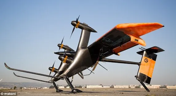
Figure 1.3: Google’s Makani tethered wind turbine.

Source: “http://www.google.com/makani/”

(c) NASA's distributed electric propulsion:This prototype from NASA makes use of ten propellers mounted on its wing and tail. As can be seen from Figure 1.4, majority of the wing and tail lie in the slipstream of the propellers. With V/STOL capabilities, aircraft similar to this prototype are expected to replace the current conventional aircraft in near future [21] .

Figure 1.4: NASA's multipropeller aircraft.

Source: “http://www.nasa.gov/aero/nasa-moves-to-begin-historic-new-era-of-x-plane-research”

pro-peller disk area. There is an increased dynamic pressure throughout the slipstream. From exper-iments in [22], [23], and numerous other references and CFD simulations in [20], it is observed that the lift on the wing increases due to the interaction. Hence the aerodynamics and flight dynamics of aircraft could be optimized to make use of this beneficial slipstream lift enhance-ment.

1.2.3 Background for propeller-slipstream/wing interaction

There has been great interest in understanding the flow behind a propeller and its effects on the wing’s performance since the early 1900s when experiments were conducted and theories proposed to study the same [22] [24] [25]. Since fighter planes were all powered by propeller propulsion, much research during this period was focused on understanding and improving pro-peller performance. Early work of Goldstein in [24] lay the foundation for theoretical models of screw propellers. In this paper the propeller blades were modeled using a single bound vortex leg spanning the length, much like the lifting line theory (LLT) for wings [26]. Research in ([20], [22], [27], [28], and numerous others) deals with understanding the propeller slipstream. Robin-son et al. in [29] conducted experiments on wing-nacelle-propeller interference and measured the spanwise distribution of pressure, which indicated that beyond two propeller diameters or five nacelle diameters in the lateral direction, their respective influence on the wing can be neglected. Smelt et al. in [30] derived an empirical relation based on momentum theory and magnetic shell theory to estimate the lift coefficient increment of a wing influenced by propeller slipstream. Experiments were also conducted to measure the lift and the velocity distribution along the slipstream. The empirical relations gave an agreeable estimation of lift increment when compared to the experimental results. These empirical relations ignored the tangential and radial components of slipstream velocity.

Experiments by Stuper in [22] showed a general increase in wing lift coefficient with the introduction of propeller slipstream and a simple jet with no tangential or radial velocity com-ponents. These experimental results were compared with those from a modified lifting-line model of the wing in [31] by Hunsaker et al. for the simple jet cases. The results match moderately well below the stall angle of the airfoil.

Effect of propeller slipstream on performance of stability of aircraft were studied separately by Butler et al. in [32], Obert in [33] and Weil et al. in [34]. Custers in his 1996 paper [35] detailed the results of experiments on aircraft half models under propeller influence and found that the drag of the model decreased and lift increased under propeller influence.

Numerous experimental and theoretical studies were conducted on understanding and esti-mating the effect of propeller slipstream on the wing and vice versa ([38, 39, 40, 41, 42, 43, 44, 45, 46, 47].) Most extensive study of the interaction was conducted by Veldhuis [20], wherein both numerical modeling and experimental analysis was undertaken. The effects of propeller position with respect to the wing, nacelle influence and ways to optimize the gain from the interaction are also studied. Ananda et al. in [48] and [49] conducted experimental studies on the propeller influence on rectangular wings of different aspect ratios at various advance ratio values of the propeller. Recent studies have been focused on the effect of propeller slipstream on the aerodynamic characteristics of Micro Air Vehicles (MAV) ([50], [51] and [52]).

1.2.4 Motivation

As seen in section 1.2.3, extensive work has already been done to estimate the effect of propeller slipstream on wings. Numerical methods, including high-fidelity CFD simulations, were also used for understanding the interaction better. These methods, though accurate, require a large number of input variables to define the wing model, computational power or both. In the current research, attempts are made to employ analytical tools for estimating the propeller slipstream velocity data, in conjunction with low-order wing modeling to estimate the propeller slipstream effect on the wing.

1.3

Outline of the thesis

Chapter 2

Low-order modeling of wing with

upstream flow disturbances

Low-order models are simplified numerical methods which are computationally less expensive than CFD simulations. These models require orders of magnitude less time to run and give a less accurate solution to those from CFD simulations. The challenge with the development of low-order methods is to effectively simulate the most essential flow effects, so that the method is suitable for initial design phases of aircraft and controller development

The low order method used in the current work builds on Weissinger's lifting line formulation [53], which is a simplified Vortex Lattice Method (VLM). This method is used extensively for wing design in situations where inviscid analysis is sufficient. In the current work, the method is extended to handle upstream flow disturbances due to (i) streamwise-oriented vortex impingement and (ii) propeller slipstream impingement on a wing. The aim is to determine if the results from the extended Weissinger method compare well with CFD and experimental data in the literature. This chapter briefly presents the methodology for the Weissinger formulation along with the extensions to handle the upstream disturbances.

2.1

Weissinger

'

s method

Weissinger's lifting line method is employed to model the wing in the current research. This method is an extension of Prandtl's lifting line theory [54]. This low-order method is inviscid, i.e., it cannot capture the viscous flow effects like boundary layer formation, flow separation, etc. and cannot predict skin friction drag on the wing.

In this method, the wing is discretized into several lattices, each having a horseshoe vortex of unknown strength Γi, where iis the index of the section, whose value ranges from 1to Ntot,

Figure 2.1: Weissinger’s discretization on a swept wing.

Source: [55]

The horseshoe vortex has a bound vortex and two trailing vortices. The bound vortex is placed at the 1/4th-chord (quarter-chord) point of the panel, while the trailing vortices extend to downstream infinity. A control point is located at the 3/4th-chord location of each panel. The Trefftz plane is located at an infinite distance downstream and its normal is parallel to the freestream velocity. The Trefftz plane analysis yields the induced drag on the wing.

Downwash due to each of the limbs of the horseshoe vortices is calculated at each control point using the Biot-Savart law.

d~V = Γ 4π

d~l×~r

|~r|3 (2.1)

where d~V is the induced velocity vector at a point due to vortex filament of length d~l, ~r is the perpendicular distance of the point from the filament and Γ is the vortex strength of the filament.

Thus the contribution of induced velocity due to each unit-strength horseshoe vortex at each control point and at each Trefftz-plane control point gives two influence coefficient matrices, aerodynamic influence coefficient matrix [A] and Trefftz-plane influence coefficient matrix [Ft].

{Vin,t}= [Ft] {Γ} (2.3)

Based on the geometric angle of attack of the wing (α), twist at the section (θ), and zero lift angle of attack of the section (α0l), the flow-tangency boundary condition is applied at the

control points for each section. The normal components of freestream velocity are :

{V∞n}=|V∞| {sin(α+θ−α0l)} (2.4)

where|V∞|is the magnitude of the freestream velocity.

Combining Eq. 2.2 and Eq. 2.4 we have

{Vin}= [A] {Γ}=V∞{sin(α+θ−α0l)} (2.5)

The resulting system of linear equations is solved using a conjugate gradient matrix solver [56]. The solution to this system gives the circulation strengths of horseshoe vortices at each panel of the wing.

Kutta-Jukowski theorem is applied to find the sectional lift contributions of the panel as

dLi=ρ ViΓidsi (2.6)

where V and ds are the total velocity and length of the ith panel of the wing respectively. Spanwise lift coefficients are calculated by non-dimensionalizing the sectional lift forces obtained from Eq. 2.6 as follows:

Cli=

dLi

1

2ρV∞2cidsi

(2.7)

CL= Ntot X i=1 dLi 1 2ρV∞2S

(2.8)

Substituting the circulation strengths in Eq. 2.3 gives the Trefftz-plane induced velocities. These velocities can be used to find the total induced drag force on the wing as:

Di = Ntot

X

i=1

ρ

2ΓiV(in,t)idsi (2.9)

Weissinger's method, the core of the simulation, is coded in FORTRAN 95 [57] using gfortran [58] compiler. The FORTRAN code needs specifications of the wing to discretize it geometrically along with the freestream velocity (V∞). The input parameters for the simulation include

(1) Span of the wing (b)

(2) Area of the wing (S)

(3) Reference span (bref), chord (cref), and area (Sref) of the wing

(4) Sweep angle of the wing at quarter chord (Λ)

(5) Number of sections of the wing

(6) Number of panels in each section of the wing

(7) Coordinates of leading edge of both ends of each section of the wing along the three coor-dinate axes.

(8) Chord length at each end of each section (c) (chord length is linearly interpolated between the ends of the section)

(9) Twist at each end of each section (θ) (twist angle is linearly interpolated between the ends of the section.)

(10) Zero lift angle of attack at each end of each section

This data is read by the FORTRAN code from an input file and stored in several vectors. Unlike Prandtl's lifting line method, Weissinger's lifting line method can model wings with sweep and dihedral angles. Weissinger's model takes in the number of sections of the wing, end coordinates of each section, twist distribution, zero lift angle of attack distribution along each section of the wing, and geometric angle of attack of the wing. Weissinger's method models the horseshoe vortices as rigid vortices, i.e., the strength and shape of these vortices remain constant and it is assumed that the wake does not roll up.

For the following sections, MATLAB [59] handles pre-processing and post-processing of data. It is within a MATLAB code that XFOIL [60] and XROTOR [61] analysis tools and the FORTRAN code are run.

2.2

Modification to Weissinger

'

s method to handle vortex

im-pingement on a wing

In this section of the thesis, the procedure followed for simulation of vortex impingement on wing is detailed. The vortex being considered in this work is the Q-vortex and the velocities induced by this vortex are as follows:

ux(r) = 1−∆ue−(r/r0)

2

(2.10)

uθ(r) =

q∆u r/r0

(1−e−(r/r0)2) (2.11)

ur(r) = 0 (2.12)

q = Γ0

2πr0∆u

≈1.567V0

∆u (2.13)

whereux is the axial component of induced velocity,uθ is the tangential component of induced

velocity, ur is the radial component of velocity, assumed to be zero in our case,q is the swirl

parameter, ∆u is the axial velocity deficit in the vortex core of radius r0, Γ0 is the vortex circulation and r is the radial distance from the center of the vortex and V0 is the maximum circumferential velocity. Further details of these equations are discussed in Chapter 3.

For the case of vortex impingement on a wing, specifications of the vortex such as, strength, radius, position of the vortex, etc. are read from a separate input file into the FORTRAN code.

Wing specifications and working conditions Vortex specifications MATLAB (pre-processing of data) FORTRAN Code MATLAB (post-processing of data) Plots input file results

Figure 2.2: Flow chart for streamwise-oriented vortex impingement on a wing

initial freestream velocity vector as follows:

~

V_i0 =V∞ˆi+ (u(x)iˆi+u(θ)iˆj) (2.14)

where, u(x)i and u(θ)i are the axial and tangential components of induced velocity due to the

impinging vortex and V~_i0 is the resultant velocity vector at ith station which is taken as the new input velocity for the Weissinger method. Equation Eq. 2.14 is only valid for planar wings encountering Q-vortices that are in the plane of the wing.

Equation 2.4 now becomes

V_n0 =|V0|nsin(α+θ−α0l+ tan−1

w u)

o

(2.15)

values. These values of circulation strengths are used to compute the aerodynamic coefficients. This process is repeated for all the angles of attack with the step size provided. The coefficients are then written to file and read by MATLAB for further processing and plotting.

2.3

Modification of Weissinger

'

s method for handling the

propeller-slipstream impingement on a wing

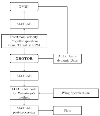
A similar procedure described in section 2.2 is followed to input wing data and discretize the wing. Instead of inputting the vortex specifications, the freestream velocity and the induced velocities from propeller slipstream are directly read into the FORTRAN code. The induced velocities are obtained from XROTOR propeller analysis tool in terms of axial and tangential components. These components are read into the FORTRAN code and a resultant velocity vector is calculated at the sections of the wing, within one radius distance from the position of the propeller disk as follows:

~

V_j0 =V∞ˆi+ (u(x)jˆi+u(θ)jˆj) (2.16)

where j = 1, 2, 3....2Nb, Nb being the number of sections along one blade. Flow tangency

boundary condition, similar to that in section 2.2, is applied as follows:

V_n0 =|V0|nsin(α+θ−α0l+ tan−1

w u)

o

(2.17)

This formulation assumes that the propeller hub is situated at the same vertical position as the wing and that the slipstream does not deflect. The rigid vortex assumption is reasonable for this inviscid analysis.

To obtain the induced velocities from XROTOR, a methodology similar to that described in Marshall’s report [62] for propeller design and analysis is adopted and is as follows:

(i) Propeller specifications (diameter, blade airfoil shape, pitch angle along the blade, chord length along the blade and RPM) are read into MATLAB.

(ii) Propeller blade is discretized into several sections (a minimum of 10 are required.)

(iii) From chord length, freestream velocity and RPM of the propeller, the Reynolds number at each of the sections is calculated.

(iv) knowing the shape of the propeller blade, XFOIL airfoil analysis tool is run for all the sections to estimate the following parameters

(2) Cd

(3) Cm

(4) dCl/dα

(5) Cl,max

(6) Cl,min

(7) Cd,min

(8) Cl atCd,min

(9) dCd/dC_l2 and

(10) Mcrit

(v) With this information, a new propeller is built from scratch using the ARBI command. Number of blades, freestream velocity, hub radius etc. are input along with the sectional aerodynamic data obtained earlier.

(vi) Thrust (T) and RPM or RPM and advance ratio (σ) are given as the operating conditions of the propeller to calculate the induced velocities.

(vii) These induced velocities are saved to file and read into MATLAB.

(viii) MATLAB discretizes the wing into the specified number of panels and interpolates the induced velocities within the diameter of the propeller which is written to file.

(ix) These interpolated velocities are read by the FORTRAN code and added to the initial freestream velocity.

(x) A similar procedure as detailed in section 2.2 is followed hereafter to compute the circu-lation strengths and aerodynamic coefficients.

(xi) The procedure is repeated several times depending on the number of angles of attack of the wing to be simulated.

(xii) If a propeller and wing combined pitch is needed, a component of the freestream velocity along the inclined propeller is taken as the new freestream and the entire procedure from step i to step xi is followed.

XFOIL

MATLAB

Freestream velocity, Propeller specifica-tions, Thrust & RPM

XROTOR _{dynamic Data}Airfoil

Aero-MATLAB

FORTRAN code for Weissinger's

method

Wing Specifications

MATLAB

post-processing Plots

Figure 2.3: Flow chart for handling propeller-slipstream impingement on a wing

Chapter 3

Results and comparisons

This chapter deals with the discussion of results obtained from low-order modeling of the wing and comparison of these results with those from the existing literature. Section 3.1 describes the results obtained from the low-order model of the wing using the modified Weissinger's method with a vortex impinging on the wing. Section 3.2 provides details of the results from simulations of propeller-slipstream impingement on a wing obtained from the modified Weissinger method and also compares these results to those in the literature.

3.1

Streamwise-oriented vortex impingement

Low-order modeling of wing for formation flight simulations has been in practice for many decades. Ever since modern computer methods came into existence, there has been a desire to understand the benefits of formation flight and several studies were conducted in both com-putational and experimental investigations. The motivation for the exploration of vortex im-pingement on a wing using low-order models in the current work is the recent availability of high fidelity CFD data on the aerodynamic performance of a wing with a streamwise-oriented vortex impingement.

3.1.1 CFD results from literature

ux(r) = 1−∆ue−(r/r0)

2

(3.1)

uθ(r) =

q∆u r/r0

(1−e−(r/r0)2) (3.2)

q = Γ0

2πr0∆u ≈1.567 V0

∆u (3.3)

whereux is the axial component of induced velocity,uθ is the tangential component of induced

velocity, q is the swirl parameter, ∆u is the axial velocity deficit in the vortex core of radius

r0, Γ0 is the vortex circulation, and r is the radial distance from the center of the vortex. For the current study q= 2, ∆u= 0.4V∞ , V0 = 0.5V∞, andr0 = 0.1cwere chosen, where c is the chord length of the wing,V0 is the maximum circumferential velocity, andV∞is the freestream

velocity.

Figure 3.1: The (i) top view and (ii) side view of the CFD simulation setup from the reference paper [14].

Source: [14]

Sectional wing lift coefficient data is provided for two cases of vortex impingement namely, (i) Inboard impingement and (ii) Tip impingement. Inboard impingement of vortex is when the Q-vortex impinges the wing at 2/3rd _{semi-span from the center of the wing. For the case of}

tip impingement, the vortex was positioned at the wing-tip. The results from these cases were compared to the baseline model with no vortex impingement.

Figure 3.2: Comparison of sectional lift coefficient for (1)Baseline, (2)Tip-impingement of vor-tex and (3)Inboard impingement of vorvor-tex cases from CFD data [14]

Figure 3.2 shows the sectional lift coefficient distribution for the cases of baseline, inboard impingement, and tip impingement obtained from the CFD simulation data. As expected, the sectional lift coefficient values are higher all along the span of the wing for both cases of vortex impingement when compared to the baseline case. The outboard portion of the wing, where the vortex impinges, has close to zero sectional lift coefficient values which increase to a maximum just inboard of the vortex impingement. There also seems to be a sharp increase in lift coefficient values within a small region around the vortex position which, the low-order model fails to capture.

For simplicity, a chord length of 1 m and a span of 6 m are assumed and the freestream velocity calculated accordingly from the Reynolds number provided. The wing is discretized into 600 panels along the span. The following are the results obtained from the low-order method as compared to the CFD data.

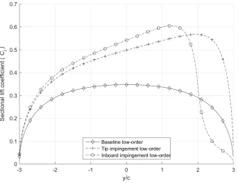
Figure 3.3: Comparison of sectional lift coefficient for (1) Baseline, (2) Tip-impingement of vortex and (3) Inboard impingement of vortex cases from low-order method

Figure 3.3 shows the comparison of sectional lift coefficient distribution along the span of the wing from the low-order model for the three cases of baseline, tip impingement, and inboard impingement. As can be observed, there is an increase in the value of sectional lift coefficient throughout the span of the wing for both positions of the impinging vortex. The inboard impingement of vortex produces downwash on the outboard portion of the wing where the vortex impinges and the sectional lift coefficient goes to a very low value in this region. The sectional lift coefficient peak is higher in the case of inboard impingement. The trends are similar to those seen from the CFD results.

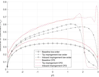
Figure 3.4: Comparison of sectional lift coefficient for (1) Baseline, (2) Tip impingement of vortex and (3) Inboard impingement of vortex cases from CFD data and low-order model results

lift coefficient data for all the cases considered. The low-order model results seem to follow the trend of the CFD results but vary quantitatively. This quantitative mismatch might be due to the laminar separation bubble formation on the wing all along the span leading to an effective change in camber of the wing. Garmann and Visbal [14] also describes a dynamic vortex phenomenon called vortex bifurcation, wherein the vortex divides into two smaller vortices one flowing above the wing and one below the wing, for the inboard impingement case. For the tip impingement case, the vortex seems to interact with wingtip vortex which is not captured by the low-order method.

Since the absolute value of sectional lift coefficients do not match and since the low-order model predicts the trends moderately well, comparison of change in sectional lift coefficients due to the vortex impingement is carried out. Figures 3.5 and 3.6 show the comparison of change in sectional lift coefficient due to vortex impingement on the wing. From Figure 3.5 we see that the sectional lift coefficient values increase as we move from left to right along the span of the wing and CFD data shows a peak value of around 0.7 while the low-order model predicts a peak of only 0.3. This discrepancy can be attributed to the interaction of the impinging vortex with the wingtip vortex. From Figure 3.6 we see that the change in sectional lift coefficient values match very well for the inboard impingement of vortex and there seems to be a slight mismatch around the vortex position and more near the wingtip. These plots explain the mismatch in rolling moments from the results for low-order method and CFD simulations.

Figure 3.5: Comparison of change in sectional lift coefficient for tip impingement of vortex from low-order model and CFD data

Figure 3.6: Comparison of change in sectional lift coefficient for inboard impingement of vortex from low-order model and CFD data

Figure 3.7: Comparison of change in sectional lift coefficient for inboard and tip impingement of vortex from both the low-order model and CFD data.

3.2

Propeller-slipstream impingement on a wing

As we already saw from Section 1.2.3, numerous experiments were conducted to understand the effect of propeller-slipstream impingement on a wing ever since propeller powered planes came into existence. With the advance of technology and the need to cut down on fossil fuel consumption, there has been an increased interest in understanding propeller-slipstream/wing interaction. The motivation for this research is the aim to model this interaction efficiently at a fraction of computational cost of a CFD simulation and to conveniently modify wing designs, which is advantageous for initial design phases of aircraft development.

3.2.1 Results from Experiments

fol-lowing cases, where propeller slipstream velocity distribution has been measured, the induced velocity data is used directly as an input to the FORTRAN code. In cases where the slipstream velocity information is not available, XROTOR analysis tool is used to calculate the induced velocity data inside the propeller slipstream in cases when propeller dimensions are specified.

3.2.1.1 Case study 1

For this case study, the experimental work by Stuper in his 1938 paper [22] is considered. The experimental setup consists of a rectangular wing with a chord of 20 cm, a span of 80 cm with a G¨ottingen 409 airfoil cross-section inside a low-speed wind tunnel operating at a freestream velocity of 30 m/s. As can be seen from Figure 3.8, the experimental setup employs circular end plates at either end of the finite wing. In this experiment the propeller is kept stationary while the wing alone is pitched to change the AoA.

Figure 3.8: Experimental setup showing the wing with circular end plates behind a propeller in a wind tunnel.

Source: [22]

were studied with the propeller running at various advance ratios with respect to the freestream velocity. For the case of axial jet flow impingement, two axial jet velocities of 118% and 136% freestream velocity (an increment of 5.4 m/s and 10.8 m/s compared to the freestream velocity, respectively) were considered. The wing in this experiment is divided into several sections each having an array of pressure probes to compute the pressure distribution on the section. Total wing lift coefficients and sectional lift coefficients at angles of attack of 4 degrees, 8 degrees, and 12 degrees are provided for the cases of axial jet flow impingement. Specifications of the propeller are also provided.

In the current research the influence of axial jet impingement on the wing is simulated using a modified Weissinger method. The freestream velocity data including the axial jet velocities is provided for the two cases (18% increment and 36% increment) and hence is directly inputted into the FORTRAN code. A recent paper by Hunsaker ([31]) also compares these experimental results to a modified panel method coupled with airfoil numerical solver. Since end plates were employed in the experiment, simulations were run with various sizes of end plates to match the baseline wingtip sectional lift coefficient for the case of AoA of 4 degrees and an end plate length of 12 cm extending in both the positive and negative “z” directions is chosen. The choice of angle of attack of 4 degrees to match the sectional lift coefficients is to ascertain no separation of flow on the wing. Simulations were run up to an angle of attack of 12 degrees.

The results from the simulations are as follows:

In this case the baseline wing model is tested at various angles of attack with a normalized velocity Vjet/V∞ of 1 inside the jet and the sectional and total wing lift coefficients obtained

are compared with those from the experiments.

Figure 3.9: Case 1A: Comparison of sectional wing lift coefficients for AoA of 4 degrees, 8 de-grees, and 12 degrees from low-order model and experimental data from [22] with no jet im-pingement

Case 1B

In this case an axial jet of velocity 35.4 m/s, normalized velocityVjet/V∞ of 1.18 within the jet,

is impinged on the wing and the sectional and total lift coefficients are compared. Figure 3.11 compares the Cl distributions and Figure 3.12 compares the lift curves. Again, it is seen that

the results from the low-order method compare well with the experimental results, except for the deviation at AoA of 12 degrees.

Figure 3.12: Case 1B: Comparison of total wing lift coefficients for AoA of 0 degrees to 12 de-grees from low-order model and experimental data from [22] with 18% jet impingement

Case 1C

In this case an axial jet of velocity 40.8 m/s, normalized velocity Vjet/V∞ of 1.36 within the

jet, is impinged on a wing and the sectional and total lift coefficients are compared. Figure 3.13 compares the Cl distributions and Figure 3.14 compares the lift curves. Again, it is seen that

We see that the total wing lift coefficients from the low-order model match very well with the experimental data up to an AoA of 10 degrees for both cases of jet impingement. As the wing approaches an AoA close to the stall angle of the airfoil, the low-order model over-predicts the lift coefficients. As explained in [22], there seems to be a velocity deficit behind the walls of the jet due to viscous flow effects and is seen as a depression about the center of the wing. As expected, the slope of wing lift curve increases with an increase in the jet velocity as seen in Figure 3.15.

3.2.1.2 Case study 2

For this case study, the experimental work by George and Kisielowski [63] is considered. Fig-ure 3.16 describes the experimental setup.

Figure 3.16: Sketch of experimental setup with the fuselage half-model.

Source: [63]

In this experiment a rectangular semi-span wing with an NACA0015 airfoil cross-section attached to a fuselage half model is tested in a low-speed wind tunnel with a propeller attached to it at the center of the semi-span from 0 degrees to 90 degrees AoA. The chord and span of the wing are 45 cm and 290 cm respectively. Propeller slipstream influence on wing performance is studied by experimenting with slipstream from two separate propellers at various advance ratios including a few at the propeller windmilling state. A constant Reynolds number of 0.8×106 is maintained within the propeller slipstream.

follows:

CTs = Tp

QsAp

(3.4)

where Tp is the thrust produced by the propeller,Ap is the propeller disk area (πR2p), andQs

is defined as

Qs=Q0+

Tp

Ap

(3.5)

Q0 being the freestream dynamic pressure. The results provided include the total wing lift coefficient values for one of the propellers with the propeller slipstream impinging on the wing. This report provides the specifications of the propeller and the working conditions and hence XROTOR analysis tool is used to compute the propeller-slipstream induced velocities. Low-order model results for the case of no propeller-slipstream impingement are also simulated. Two cases of the experiment are simulated and the results are plotted and discussed below.

Case 2A

In this case the propeller was run at an RPM of 2700 while maintaining a freestream velocity of 17.8 m/s in the wind tunnel. The thrust produced by the propeller was 224.1 N, which is equivalent to a thrust coefficient of 0.6. The radius of the propeller was 50 cm. A constant slipstream Reynolds number of 0.8×106 is maintained. Simulations were run for AoA from 0 degrees to 40 degrees. Simulations were also run for no propeller impingement case at these operating conditions and are co-plotted in Figure 3.17. From the results obtained, we see that the low-order method gives accurate results for up to an AoA of 12 degrees beyond which it over-predicts. Simulation results for the no vortex impingement case show that the lift curve slope increases with the introduction of propeller slipstream.

Case 2B

Figure 3.17: Case 2A: Comparison of total wing lift coefficient results from low-order methods to the experimental data atCTs = 0.6

Figure 3.18: Case 2B: Comparison of total wing lift coefficient results from low-order methods to the experimental dataCTs = 0.93.

3.2.1.3 Case study 3

of 20.32 cm and a span of 81.28 cm with an NACA 64A418 airfoil cross-section is tested in a low-speed wind tunnel under the influence of a propeller with a diameter of 20.32 cm and unknown geometry. The wing is divided into 19 unequal sections each with a separate sting balance to measure the forces.The wing is not attached to the propeller and the propeller is maintained at a constant pitch angle while the wing alone is pitched up or down. An average dynamic pressure, ˆq, defined as

ˆ

q= q0+qj

2 (3.6)

is used to non-dimensionalize the forces to obtain the coefficients, where q0 is the freestream dynamic pressure, qj = q0+ ∆q, and ∆q is the average increment in dynamic pressure within

the slipstream defined as

∆q = 2

R2

p

Z Rp

0

y(qj−q0)dy (3.7)

Here qj is the dynamic pressure at a radial section along the propeller blade. This experiment

Figure 3.19: Experimental setup of the propeller and wing inside the subsonic wind tunnel.

Source: [23]

are directly inputted into the FORTRAN code for modified Weissinger method.

Since the wing spans the entire height of the wind tunnel, endplates of length 2 m are used on either side of the wing in the simulations. This length was chosen to equate the baseline wingtip sectional lift coefficients for 6.5 degrees for Case 3A. The force coefficients are obtained by non-dimensionalizing the forces obtained by the above defined dynamic pressure which is calculated for each case of freestream dynamic pressure. Since the Reynolds number in the wind tunnel changes, the zero-lift angle of the wing sections also changes. XFOIL analysis tool is run at Reynolds numbers corresponding to each case of freestream dynamic pressure to determine the zero-lift AoA to input to the FORTRAN code.

Case 3A

In this case the freestream dynamic pressure in the wind tunnel is maintained at 1.55 in of EG and the wing is tested at an AoA of 6.5 degrees and 11.5 degrees. The freestream veloc-ity is 26.5 m/s and Reynolds number is 451,516. The zero-lift AoA obtained from XFOIL is −2.9 degrees. From Figures 3.19 and 3.20 we see that the baseline sectional lift coefficient from the experiment matches with the low-order model lift coefficient at the wingtips, as expected from the discussion above, since the endplate size is determined in such a way so as to equate the wingtip sectional lift coefficients values. In both cases the low-order method predicts Cl

Case 3B

In this case the freestream dynamic pressure in the wind tunnel is maintained t 0.69 in of EG and the wing is tested at an AoA of 6.5 degrees and 11.5 degrees. The freestream velocity is 17.7 m/s and Reynolds number is 301,328. The zero-lift AoA as obtained from XFOIL is −2.9 degrees. Figures 3.21 and 3.22 detail the plots for the comparison of sectional lift coefficients for angles of attack of 6.5 degrees and 11.5 degrees from experimental results and low-order method predictions. The predictions seem to match well with the CFD results with the exception of the two troughs beside the propeller slipstream apparently from the viscous flow effects of the propeller slipstream boundary. It can also be observed that as the AoA increases the predictions become less accurate.

Figure 3.23: Case 3B: Comparison of sectional lift coefficients from low-order method and experimental data for an AoA of 11.5 degrees at a freestream dynamic pressure of 0.69 in of EG

Case 3C

Case 3D

In this case the freestream dynamic pressure in the wind tunnel is maintained at 0.19 in of EG and the wing is tested at an AoA of 6.5 degrees and 11.5 degrees. The freestream velocity is 9.26 m/s and Reynolds number is 157,953. The zero-lift AoA as obtained from XFOIL is −2.7 degrees. For this case, as can be seen from figures 3.25 and 3.26, the predictions do not match the experimental results but give a qualitative description.

Figure 3.27: Case 3D: Comparison of sectional lift coefficients from low-order method and experimental data for an AoA of 11.5 degrees at a freestream dynamic pressure of 0.19 in of EG

From the plots above we see that the low-order model predicts the peak of the sectional lift coefficient very well but fails to capture the loss in lift around this central peak which, is present in all the experimental data provided. We also see that, as the AoA is increased from 6.5 degrees to 11.5 degrees the accuracy of the low-order model decreases. This is because the wing approaches the airfoil stall angle where the low-order model fails to predict the lift coefficients accurately. We also see that as the freestream dynamic pressure decreases, the accuracy of the results decreases with the data at a freestream dynamic pressure of 1.55 in of EG being the most accurate and the data at a freesream dynamic pressure of 0.19 in of EG being the least.

Chapter 4

Conclusions

4.1

Conclusions

Upstream flow changes or disturbances alter the inflow conditions of a wing. These changes in the inflow conditions affect the aerodynamic performance of the wing. In this thesis, the focus is on the effects on a finite wing encountering (1) a streamwise vortex, similar to that generated by the wingtip of an upstream aircraft and (2) a propeller slipstream. The current thesis deals with modeling these effects using low-order methods for wing and comparing the results with experimental and computational data from the literature. From the comparisons in Chapter 3 we see that the Weissinger's low-order method performs well at low angles of attack and at higher Reynolds numbers where flow separation is unlikely. This is due to the inviscid nature of the method. As mentioned earlier, this research aims to employ the already existing airfoil and propeller analysis tools XFOIL and XROTOR to model the propeller induced flow effects to save on computational power and time consumption and to reduce the simulation complexity. We see from the results in Chapter 3, this low-order models predicts the lift data agreeably well and the wing geometry changes can be made effortlessly.

From the analysis and comparison in the previous chapters, the following are the advantages of the Weissinger's low-order model, in conjunction with the XFOIL and XROTOR analysis tools, followed in this research: (i) computationally less expensive, (ii) wing shape can be mod-ified easily and with minimum number of inputs, (iii) wings with sweep and dihedral can be modeled, and (iv) gives a general idea of influence of upstream flow disturbances on wing perfor-mance for initial design of aircraft development. The disadvantages are: (i) wing model cannot capture viscous flow phenomenon, (ii) results are only agreeably accurate up to and below the stall angle of each section of the wing, and (iii) cannot simulate wing influence on propeller (full interaction mode) and in turn the effect on wing performance.

analysis tools and post-processing of data using MATLAB is in the order of a few hundred (≈300−500) seconds when the panel density is 1000 per one meter of the wing span for a span of 80 cm. If the propeller slipstream data is readily available, the simulation time reduces to a few (≈8−10) seconds for a complete run. Here a complete run indicates a simulation for 10 angles of attack. From the results it can be concluded that the low-order model predictions are reasonably accurate at handling the inflow disturbances provided the wing is operating well below the stall angle and when the viscous effects of flow and complex vortex dynamics are not in play. From this work it can be concluded that low-order models could be employed to effectively simulate upstream flow disturbances on aerodynamic performance of a wing, operating at attached flow conditions, with a fraction of computational cost of a CFD simulation.

4.2

Future work

REFERENCES

[1] Thomas Gerz, Frank Holz¨apfel, and Denis Darracq. Commercial aircraft wake vortices. Progress in Aerospace Sciences, 38(3):181–208, 2002.

[2] Thomas Gerz, Frank Holz¨apfel, Wayne Bryant, Friedrich K¨opp, Michael Frech, Arnold Tafferner, and Gr´egoire Winckelmans. Research towards a wake-vortex advisory system for optimal aircraft spacing. Comptes Rendus Physique, 6(4):501–523, 2005.

[3] George C Greene. An approximate model of vortex decay in the atmosphere. Journal of Aircraft, 23(7):566–573, 1986.

[4] Turgut Sarpkaya. New model for vortex decay in the atmosphere. Journal of Aircraft, 37(1):53–61, 2000.

[5] PBS Lissaman and Carl A Shollenberger. Formation flight of birds. Science, 168(3934):1003–1005, 1970.

[6] Airbus global market forecast 2015-2034, 2015.

[7] Boeing commercial airplanes, current market outlook 2015-2034, 2015.

[8] Donald Rockwell. Vortex-body interactions. Annual review of fluid mechanics, 30(1):199– 229, 1998.

[9] Dietrich Hummel. Aerodynamic aspects of formation flight in birds. Journal of theoretical biology, 104(3):321–347, 1983.

[10] Dietrich Hummel. Formation flight as an energy-saving mechanism. Israel Journal of Zoology, 41(3):261–278, 1995.

[12] Henri Weimerskirch, Julien Martin, Yannick Clerquin, Peggy Alexandre, and Sarka Ji-raskova. Energy saving in flight formation. Nature, 413(6857):697–698, 2001.

[13] Ayumu Inasawa, Fumihide Mori, and Masahito Asai. Detailed observations of interactions of wingtip vortices in close-formation flight. Journal of Aircraft, 49(1):206–213, 2012.

[14] Daniel J Garmann and Miguel R Visbal. Interactions of a streamwise-oriented vortex with a finite wing. Journal of Fluid Mechanics, 767:782–810, 2015.

[15] Caleb J Barnes, Miguel R Visbal, and Raymond E Gordnier. Analysis of streamwise-oriented vortex interactions for two wings in close proximity. Physics of Fluids (1994-present), 27(1):015103, 2015.

[16] James W Frazier and Ashok Gopalarathnam. Optimum downwash behind wings in for-mation flight. Journal of Aircraft, 40(4):799–803, 2003.

[17] Rachel M King and Ashok Gopalarathnam. Ideal aerodynamics of ground effect and formation flight. Journal of Aircraft, 42(5):1188–1199, 2005.

[18] John T Conway. Exact actuator disk solutions for non-uniform heavy loading and slip-stream contraction. Journal of Fluid Mechanics, 365:235–267, 1998.

[19] Theodore Theodorsen. The theory of propellers iii: the slipstream contraction with numer-ical values for two-blade and four-blade propellers. 1944.

[20] Leonardus Louis Maria Veldhuis.Propeller wing aerodynamic interference. TU Delft, Delft University of Technology, 2005.

[21] Alex M Stoll, JoeBen Bevirt, Mark D Moore, William J Fredericks, and Nicholas K Borer. Drag reduction through distributed electric propulsion. 2014.

[23] M Brenckmann. Experimental investigation of the aerodynamics of a wing in a slipstream. Technical Report 11, University of Toronto, 1957.

[24] Sydney Goldstein. On the vortex theory of screw propellers. Proceedings of the Royal Society of London. Series A, Containing Papers of a Mathematical and Physical Character,

123(792):440–465, 1929.

[25] Clark B Millikan. The influence of running propellers on airplane characteristics. Journal of the Aeronautical Sciences, 7(3):85–103, 1940.

[26] Edward Lewis Houghton and Peter William Carpenter. Aerodynamics for engineering students. Butterworth-Heinemann, 2003.

[27] Eric W M. Roosenboom, Arne St¨urmer, and Andreas Schr¨oder. Advanced experimental and numerical validation and analysis of propeller slipstream flows. Journal of Aircraft, 47(1):284–291, 2010.

[28] Li Bo, Liang Dewang, and Huang Guoping. Propeller slipstream effects on aerodynamic performance of turbo-prop airplane based on equivalent actuator disk model [j]. Acta Aeronautica Et Astronautica Sinica, 4:014, 2008.

[29] Russell G Robinson and William H Herrnstein Jr. Wing-nacelle-propeller interference for wings of various spans force and pressure-distribution tests. NACA Technical Report 569, 1937.

[30] R Smelt and H Davies. Estimation of increase in lift due to slipstream. HM Stationery Office, 1937.

[32] Lawrence Butler, KP Huang, and L Goland. An investigation of propeller slipstream effects on v/stol aircraft performance and stability. Technical Report 65-81, DTIC Document, 1966.

[33] E Obert. A method for the determination of the effect of propeller slipstream on static longitudinal stability and control of multi-engined aircraft. Delft University of Technology,

1994.

[34] Joseph Weil and William C Sleeman Jr. Prediction of the effects of propeller operation on the static longitudinal stability of single-engine tractor monoplanes with flaps retracted. Technical report, DTIC Document, 1948.

[35] LGM Custers. Propeller-wing interference effects at low speed contitions. Aspects of engine airframe integration for transport aircraft,NLR Technical Publication TP 96312 U, pages

19–1, 1996.

[36] JL Loth and F Loth. Induced drag reduction with wing tip mounted propellers. In American Institute of Aeronautics and Astronautics, Applied Aerodynamics Conference, 2

nd, Seattle, WA, volume 21, 1984.

[37] James E Brennan. Aerodynamic effects of wingtip-mounted propellers and turbines.AIAA 4th Applied Aerodynamics Conference, San Diego, CA, pages 221–228.

[38] FM Catalano. On the effects of an installed propeller slipstream on wing aerodynamic characteristics. Acta Polytechnica, 44(3), 2004.

[39] Daniel Favier, Christian Maresca, and Gilles Fratello. Experimental and numerical study of the propeller/fixed wing interaction. Journal of Aircraft, 28(6):365–373, 1991.

[41] F Moens and P Gardarein. Numerical simulation of the propeller/wing interaction for transport aircraft. Office National d Etudes et de Recherches Aerospatiales Onera-Publications-TP, (116), 2001.

[42] Dave P Witkowski, Alex KH Lee, and John P Sullivan. Aerodynamic interaction between propellers and wings. Journal of Aircraft, 26(9):829–836, 1989.

[43] JY Chiaramonte, D Favier, C Maresca, and S Benneceur. Aerodynamic interaction study of the propeller/wing under different flow configurations. Journal of Aircraft, 33(1):46–53, 1996.

[44] Richard E Kuhn and John W Draper. Investigation of the aerodynamic characteristics of a model wing-propeller combination and of the wing and propeller separately at angles of attack up to 90 degrees. NACA Report 1263, 1956.

[45] Ilan Kroo. Propeller-wing integration for minimum induced loss. Journal of Aircraft, 23(7):561–565, 1986.

[46] Guowei Yang and Fengwei Li. Numerical analysis of the interference effect of propeller slipstream on aircraft flowfield. Journal of Aircraft, 35(1):84–90, 1998.

[47] Ingemar Samuelsson. Low speed wind tunnel investigation of propeller slipstream aerody-namic effects on different nacelle/wing combinations. InICAS, Congress, 16 th, Jerusalem, Israel, pages 1749–1765, 1988.

[48] Gavin K Ananda, Robert W Deters, and Michael S Selig. Propeller-induced flow effects on wings of varying aspect ratio at low reynolds numbers. AIAA Aviation 16-20 June 2014, Atlanta, GA, 32nd AIAA Applied Aerodynamics Conference, 2014.

[50] Kwanchai Chinwicharnam, David Gomez Ariza, Jean-Marc Moschetta, and Chinnapat Thipyopas. Aerodynamic characteristics of a low aspect ratio wing and propeller interaction for a tilt-body mav. International Journal of Micro Air Vehicles, 5(4):245–260, 2013.

[51] Arivoli Durai. Experimental investigation of lift and drag characteristics of a typical mav under propeller induced flow. International Journal of Micro Air Vehicles, 6(1):63–72, 2014.

[52] Brian J Gamble and Mark F Reeder. Experimental analysis of propeller-wing interactions for a micro air vehicle. Journal of Aircraft, 46(1):65–73, 2009.

[53] J Weissinger. The lift distribution of swept-back wings. NACA Technical Memorandum No.1120, 1947.

[54] John David Anderson Jr. Fundamentals of aerodynamics, 2nd Edition. Tata McGraw-Hill Education, 1985.

[55] Ashok Gopalarathnam. Wing theory class notes, mae 561, 2014.

[56] Jorge Nocedal and Stephen J Wright. Conjugate gradient methods. Numerical Optimiza-tion, pages 101–134, 2006.

[57] GNU General Public License.https://en.wikipedia.org/wiki/Fortran_95_language_

features, 1995.

[58] GNU General Public License. https://gcc.gnu.org/onlinedocs/gcc-4.1.2/

gfortran/.

[59] http://www.mathworks.com/products/matlab/, 2015.

[60] Harold Youngren Mark Drela. GNU General Public License.http://web.mit.edu/drela/

Public/web/xfoil/, 2001.

[61] Harold Youngren Mark Drela. GNU General Public License.http://web.mit.edu/drela/

[62] Robert Grant Marshall. Analysis of small unmanned aerial vehicle propellers using xrotor software and investigation of experimental minimum induced loss rotors, 2015.

[63] M George and E Kisielowski. Investigation of propeller slipstream effects on wing perfor-mance. Technical Report 67-67, DTIC Document, 1967.