Compton imaging reconstruction methods: a
comparative performance study of direct
back-projection, SOE, a new Bayesian algorithm and a
new Compton inversion method applied to real data
with Caliste
G.
Daniel
1,2, O. Limousin
1, D. Maier
1, A. Meuris
1, F. Carrel
31 AIM, CEA, CNRS, Université Paris-Saclay, Université Paris Diderot, Sorbonne Paris Cité, Gif-sur-Yvette, France 2 École des Ponts ParisTech, Champs-sur-Marne)UDQFH
3 CEA, LIST, Sensors and Electronic Architectures Laboratory, Gif-sur-Yvette, France
Abstract— Compton imaging is one of the main methods to localize radioactive hotspots, which emit high-energy gamma-ray photons, above 200 keV. Most of the Compton imaging systems are composed by at least two detection layers or one 3D position sensitive detector. In this study, we demonstrate the application of a new miniature pixelated single plane detector to Compton imaging. In this configuration, we do not have the information on interaction depth but we successfully test its ability to perform Compton localization by means of comparing different Compton reconstruction algorithms applied to real data measured with our single plane detection system.
Index Terms – Compton imaging, SOE, Bayes, Caliste, Compton inversion.
I. INTRODUCTION
OMPTON imaging systems are used to localize radioactive sources which emit high-energy gamma-ray photons. This information is necessary in different domains such as nuclear safety, in accidental situations or decommissioning contexts [1], in medicine for hadron therapy dose monitoring [2] or in space observations [3] for instance.
These systems rely on the Compton scattering effect, which is the main interaction process at work for photons with an energy above 200 keV, in most of materials.
The principle of the method for gamma-ray imaging is to apply Compton kinematics [4] to find the possible origin of an impinging photon. If we note 𝐸𝐸� the initial energy of a photon,
𝐸𝐸� the energy of the scattered photon, 𝐸𝐸� the energy deposited by Compton interaction and 𝜃𝜃 the scattering angle, the energy and total relativistic momentum conservations lead to the formula:
cos(𝜃𝜃) = 1 − 𝑚𝑚�𝑐𝑐�𝐸𝐸𝐸𝐸�
�𝐸𝐸� (eq. 1)
Where 𝑚𝑚�𝑐𝑐�= 511 keV is the energy mass of an electron at rest.
Regarding the reconstruction method, Compton kinematics give only the angle 𝜃𝜃 between the direction of the original photon and the scattered photon, which gives a cone with an angle 𝜃𝜃 of possible origins in 3D.
Usual Compton imaging systems measure the Compton scattering interaction, which deposits 𝐸𝐸�, followed by the photoelectric interaction of the scattered photon.
Most of the systems use two detection layers, one scatter layer and one absorption layer, which fully absorbs the scattered photon [5]. Other systems perform Compton imaging with three or more layers, allowing reconstruction even if the final photon is not fully absorbed, assuming that the photon is scattered at least two times [6]. Finally, 3D-position sensitive systems, which are able to localize the interactions in the detector in 3D, are also used as Compton camera [7].
In this paper, we demonstrate the feasibility of Compton imaging with a single plane pixelated miniature detector, namely Caliste [8], by exploiting its advantages, especially its spectral and spatial resolution through Compton event selection. We study different Compton reconstruction algorithms to achieve the best localization performance with our detector: Direct Back-Projection (DBP) of the cones obtained by Compton kinematics, Stochastic Origin Ensemble with Resolution Recovery [9] and we introduce a new Bayesian approach and a new inversion of the Compton DBP.
Other algorithms for Compton reconstruction exist, such as Filtered Back-Projection or List-Mode Maximum Likelihood Expectation Maximization (LM-MLEM) [10]. LM-MLEM has been unsuccessfully tested for our particular detection configuration.
The paper is structured as follows:
Section II focuses on the detection system properties. Section III is dedicated to the Compton events selection. Section IV describes the different algorithms we have developed and implemented for reconstruction and Section V presents the results we get from real data acquisitions.
II. CALISTE: A MINIATURE CDTE SPECTRO-IMAGER
Caliste is a hybrid CdTe detector module, initially developed for high-energy astronomy in space, declined in different versions depending on its applications. The version used for this study is Caliste-HD [11], [12].
Caliste-HD is a pixelated imaging spectrometer made of a 16×16 pixels array with 625-μm pitch patterned on a 1 cm2
monolithic CdTe crystal, 1 mm thick. The CdTe crystal is placed on top of a 3D electronics package where eight ultra-low noise read-out ASICs IDeF-X HD [13] are embedded. In such an architecture, each pixel is a miniature and independent spectrometer channel. The package size is 10×10×16.5 mm3.
Caliste-HD performance has an excellent spectral response with 670 eV FWHM at 60 keV and 4.1 keV at 662 keV for single events in the summed spectrum of all pixels, with an energy range from 2 keV to 1 MeV for single events. An operating temperature of -10°C and an electric field of 300 V/mm are appropriate to reach these performances.
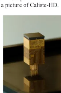
Figure 1 shows a picture of Caliste-HD.
Figure 1: Caliste-HD
We use these characteristics to perform Compton imaging with this detector integrated in a very compact system, namely WIX-HD, with a total weight of 1 kg. WIX-HD includes one Caliste-HD module installed into a small vacuum tight enclosure connected to a data acquisition electronics system. The cooling is realized by miniature thermos-electric Peltier coolers.
TABLE I
CHARACTERISTICS OF CALISTE-HD
PARAMETER CALISTE-HD
Number of pixels 256 (16×16)
Pixel Pitch 625 μm
Crystal thickness 1 mm
Dimension without
CdTe 10×10×16.5 mm3
Power
Consumption 200 mW Energy Range 2 - 1000 keV
FWHM at 60 keV 670 eV
FWHM at 662 keV 4.1 keV
This system is slightly different to the usual Compton imaging gamma-ray cameras. It is indeed composed of one planar layer of detection without interaction depth measurement, which causes disadvantages in terms of angular resolution because of the uncertainty on the interaction depth. If the two deposited energies are compatible with Compton scattering, we are not able to distinguish the Compton scattering interaction and the photoelectric absorption at first glance. Moreover, the planar configuration of our detection system implies that the detector plane is a symmetric plane in the reconstructed image, so that the field of view is not 360°×180° but 180°×180° instead.
Like every Compton imaging system, the localization resolution is essentially limited by the Doppler broadening effect [14].
However, we use the other advantages of the system, its spectroscopic performances and its small size, associated to specific algorithms, in order to perform Compton reconstruction.
III. EVENTS SELECTION
The first step of Compton reconstruction is the selection of the relevant events to perform the reconstruction. In a measurement with Caliste-HD, we first select multiple events, which are events, registered in time coincidence into the detector. The time between the Compton scattering interaction and the second interaction is indeed small compared to the time resolution of the detector of 20 μs.
The second rule is that the two events do not occur in neighbouring pixels, so that there is no possible confusion with charge sharing caused by a single interaction between the two pixels [15]. The events are also accepted if they are recorded in two separated clusters of pixels. Figure 2 shows some different and typical multiple events detection patterns.
The position in 2D associated with the events is considered to be the center of the pixel, when only single pixel hits are detected such as illustrated as type a on Figure 2. Conversely,
the interaction position is considered to be the centroid of the cluster weighted by the energy depositions in the cluster’s pixels, see Figure 2, types b and c. For instance, in the case of events type c, the centroids of each clusters are calculated separately to determine the most probable interaction coordinates in the detector array.
a b c d
Figure 2: Multiple event configurations, a: Two pixels separated, accepted pattern; b: One single pixel and one cluster, accepted pattern; c: Two clusters separated, accepted pattern; d: One cluster, rejected pattern.
Figure 3: Single-event spectrum of 137Cs source
Figure 4: Multiple events sum spectrum of a 137Cs source measurement with
Caliste-HD
Once these events are discriminated, we use energy conservation to select events with one Compton scattering interaction with an energy deposition 𝐸𝐸� and a photoelectric absorption of the scattered photon 𝐸𝐸�.
𝐸𝐸�= 𝐸𝐸�+ 𝐸𝐸� (eq. 2)
In our case, we assume having a prior knowledge of 𝐸𝐸� as a result of a spectral source identification performed on a single-event spectrum such as shown in Figure 3. This information can be obtained with a Bayesian Convolutional Neural Network [16], especially in case of small counting statistics.
Figure 4 shows a spectrum of summed multiple events, separated by at least one pixel, for a 137Cs source measurement.
The 662 keV line corresponds to reconstructed double events with a Compton scattering in the detector followed by a photoelectric absorption of the scattered photon, so that the total energy deposited corresponds to the full energy of the original photon.
The cases of single 662 keV Compton events whose scattered photons escape from the detector form the Compton edge at 478 keV as illustrated in Figure 3. However, as expected in our simulations, 662 keV double Compton events whose second scattered photon escapes from the detector tend to shift the Compton edge towards 500 keV as shown in Figure 5. In that case, the maximum reachable energy deposition is 𝐸𝐸��� = 555 keV as expressed in eq. 3.
𝐸𝐸���= 𝐸𝐸�− 𝐸𝐸� 1 + 4𝐸𝐸�
𝑚𝑚�𝑐𝑐�
(eq. 3)
Whatever the Compton interaction is, single or double, the backscatter peak remains at 184 keV for 662 keV photons emitted by a 137Cs source (eq. 4).
𝐸𝐸� = 𝐸𝐸� 1 + 2𝐸𝐸�
𝑚𝑚�𝑐𝑐�
(eq. 4)
Figure 5: Energy selection with a 137Cs source measurement on double events
Other algorithms for Compton reconstruction exist, such as Filtered Back-Projection or List-Mode Maximum Likelihood Expectation Maximization (LM-MLEM) [10]. LM-MLEM has been unsuccessfully tested for our particular detection configuration.
The paper is structured as follows:
Section II focuses on the detection system properties. Section III is dedicated to the Compton events selection. Section IV describes the different algorithms we have developed and implemented for reconstruction and Section V presents the results we get from real data acquisitions.
II. CALISTE: A MINIATURE CDTE SPECTRO-IMAGER
Caliste is a hybrid CdTe detector module, initially developed for high-energy astronomy in space, declined in different versions depending on its applications. The version used for this study is Caliste-HD [11], [12].
Caliste-HD is a pixelated imaging spectrometer made of a 16×16 pixels array with 625-μm pitch patterned on a 1 cm2
monolithic CdTe crystal, 1 mm thick. The CdTe crystal is placed on top of a 3D electronics package where eight ultra-low noise read-out ASICs IDeF-X HD [13] are embedded. In such an architecture, each pixel is a miniature and independent spectrometer channel. The package size is 10×10×16.5 mm3.
Caliste-HD performance has an excellent spectral response with 670 eV FWHM at 60 keV and 4.1 keV at 662 keV for single events in the summed spectrum of all pixels, with an energy range from 2 keV to 1 MeV for single events. An operating temperature of -10°C and an electric field of 300 V/mm are appropriate to reach these performances.
Figure 1 shows a picture of Caliste-HD.
Figure 1: Caliste-HD
We use these characteristics to perform Compton imaging with this detector integrated in a very compact system, namely WIX-HD, with a total weight of 1 kg. WIX-HD includes one Caliste-HD module installed into a small vacuum tight enclosure connected to a data acquisition electronics system. The cooling is realized by miniature thermos-electric Peltier coolers.
TABLE I
CHARACTERISTICS OF CALISTE-HD
PARAMETER CALISTE-HD
Number of pixels 256 (16×16)
Pixel Pitch 625 μm
Crystal thickness 1 mm
Dimension without
CdTe 10×10×16.5 mm3
Power
Consumption 200 mW Energy Range 2 - 1000 keV
FWHM at 60 keV 670 eV
FWHM at 662 keV 4.1 keV
This system is slightly different to the usual Compton imaging gamma-ray cameras. It is indeed composed of one planar layer of detection without interaction depth measurement, which causes disadvantages in terms of angular resolution because of the uncertainty on the interaction depth. If the two deposited energies are compatible with Compton scattering, we are not able to distinguish the Compton scattering interaction and the photoelectric absorption at first glance. Moreover, the planar configuration of our detection system implies that the detector plane is a symmetric plane in the reconstructed image, so that the field of view is not 360°×180° but 180°×180° instead.
Like every Compton imaging system, the localization resolution is essentially limited by the Doppler broadening effect [14].
However, we use the other advantages of the system, its spectroscopic performances and its small size, associated to specific algorithms, in order to perform Compton reconstruction.
III. EVENTS SELECTION
The first step of Compton reconstruction is the selection of the relevant events to perform the reconstruction. In a measurement with Caliste-HD, we first select multiple events, which are events, registered in time coincidence into the detector. The time between the Compton scattering interaction and the second interaction is indeed small compared to the time resolution of the detector of 20 μs.
The second rule is that the two events do not occur in neighbouring pixels, so that there is no possible confusion with charge sharing caused by a single interaction between the two pixels [15]. The events are also accepted if they are recorded in two separated clusters of pixels. Figure 2 shows some different and typical multiple events detection patterns.
The position in 2D associated with the events is considered to be the center of the pixel, when only single pixel hits are detected such as illustrated as type a on Figure 2. Conversely,
the interaction position is considered to be the centroid of the cluster weighted by the energy depositions in the cluster’s pixels, see Figure 2, types b and c. For instance, in the case of events type c, the centroids of each clusters are calculated separately to determine the most probable interaction coordinates in the detector array.
a b c d
Figure 2: Multiple event configurations, a: Two pixels separated, accepted pattern; b: One single pixel and one cluster, accepted pattern; c: Two clusters separated, accepted pattern; d: One cluster, rejected pattern.
Figure 3: Single-event spectrum of 137Cs source
Figure 4: Multiple events sum spectrum of a 137Cs source measurement with
Caliste-HD
Once these events are discriminated, we use energy conservation to select events with one Compton scattering interaction with an energy deposition 𝐸𝐸� and a photoelectric absorption of the scattered photon 𝐸𝐸�.
𝐸𝐸�= 𝐸𝐸�+ 𝐸𝐸� (eq. 2)
In our case, we assume having a prior knowledge of 𝐸𝐸� as a result of a spectral source identification performed on a single-event spectrum such as shown in Figure 3. This information can be obtained with a Bayesian Convolutional Neural Network [16], especially in case of small counting statistics.
Figure 4 shows a spectrum of summed multiple events, separated by at least one pixel, for a 137Cs source measurement.
The 662 keV line corresponds to reconstructed double events with a Compton scattering in the detector followed by a photoelectric absorption of the scattered photon, so that the total energy deposited corresponds to the full energy of the original photon.
The cases of single 662 keV Compton events whose scattered photons escape from the detector form the Compton edge at 478 keV as illustrated in Figure 3. However, as expected in our simulations, 662 keV double Compton events whose second scattered photon escapes from the detector tend to shift the Compton edge towards 500 keV as shown in Figure 5. In that case, the maximum reachable energy deposition is 𝐸𝐸��� = 555 keV as expressed in eq. 3.
𝐸𝐸���= 𝐸𝐸�− 𝐸𝐸� 1 + 4𝐸𝐸�
𝑚𝑚�𝑐𝑐�
(eq. 3)
Whatever the Compton interaction is, single or double, the backscatter peak remains at 184 keV for 662 keV photons emitted by a 137Cs source (eq. 4).
𝐸𝐸�= 𝐸𝐸� 1 + 2𝐸𝐸�
𝑚𝑚�𝑐𝑐�
(eq. 4)
Figure 5: Energy selection with a 137Cs source measurement on double events
As shown in Figure 5, the line shape at 662 keV is composed of three event populations: the narrow peak structure is populated with events of type a (45%) summed up with two other bumpy populations from events of type b and c. The energy of the main line emission of the source is 662 keV. Because of the slightly non-linear detector response [17] and charge loss due to split events, we use a selection window, between 647 keV and 670 keV, which is considerably larger than the detector resolution for single events. The selection is made in the main peak of the spectrum so that we keep only the best events in energy to reduce the influence of the energy uncertainty on the computation of the scattering angle 𝜃𝜃.
When these events are selected, we have to determine the order of the two measured interactions, i.e. which of the interactions is most likely corresponding to the Compton interaction. When one of the energies recorded is below the minimal energy of a Compton scattered photon 𝐸𝐸�, this interaction is associated to the Compton scattering and the other one to the photoelectric absorption.
In this case, we distinguish the two interactions. However, the Doppler broadening effect may result in an energy of the scattered photon lower than 𝐸𝐸�, which induces an error in the identification of the interaction order.
When the two deposited energies are between 𝐸𝐸� and 𝐸𝐸�−
𝐸𝐸�, we are not able to distinguish the two interactions with this rule. This situation happens when the energy of the original photon is above ����
� = 255.5 keV. One solution is to compute the two possibilities accepting that one is necessarily wrong, which causes noise in the reconstructed image, making the treatment more challenging. Alternatively, considering that the probability of photoelectric interaction is lower when the energy of the photon is higher, we attribute the photoelectric absorption to the lower deposited energy.
Writing 𝐸𝐸� and 𝐸𝐸� as the two measured energy deposits, the selection rule is:
if 𝐸𝐸�> 𝐸𝐸�− 𝐸𝐸� or 𝐸𝐸�≤ 𝐸𝐸� <���, 𝐸𝐸� is attributed to the photoelectric absorption;
otherwise, 𝐸𝐸� is attributed to the photoelectric absorption.
Eventually, the formula for Compton kinematics (eq. 1) can be used with different parameters, considering the energy conservation (eq. 2). We can use 𝐸𝐸�+ 𝐸𝐸� instead of 𝐸𝐸�, 𝐸𝐸�−
𝐸𝐸� instead of 𝐸𝐸� and 𝐸𝐸�− 𝐸𝐸� instead of 𝐸𝐸�. Analyzing the sensitivity of 𝜃𝜃 in (eq. 1) on the energy measurements 𝐸𝐸� and
𝐸𝐸� according to the different forms of the expression, we conclude that using 𝐸𝐸�− 𝐸𝐸� instead of 𝐸𝐸� leads to the minimization of the maximal error on 𝜃𝜃. Thus, we use the formula:
cos(𝜃𝜃) = 1 − 𝑚𝑚�𝑐𝑐�(𝐸𝐸 𝐸𝐸�
�− 𝐸𝐸�)𝐸𝐸� (eq. 5)
IV. RECONSTRUCTION ALGORITHMS
After Compton event selection, we perform Compton imaging using different algorithms. In this study, we have implemented four algorithms that we explain in this section and we evaluate their performance with our detector system on real data in Section V.
A. Direct Back-Projection (DBP)
Also called Simple Back-Projection, this algorithm is the direct application of the Compton kinematics. We note 𝐴𝐴, the position of the Compton interaction, 𝐵𝐵 the position of the photoelectric absorption and 𝜃𝜃 the angle computed according to equation 5. We determine the equation of the cone of axis [𝐵𝐵𝐴𝐴), of apex 𝐴𝐴 and angle 𝜃𝜃.
We compute the intersection of the cone with a sphere of radius 𝑟𝑟, where 𝑟𝑟 is the expected distance from the detector to the source. In most cases the distance is unknown and r is set to a sufficiently high value so that we consider an infinite radius length comparatively to the detector size. This intersection is called the projection of the cone.
This algorithm is applied to each individual event and the cones are added iteratively, so that we get a back-projection map in the end. For a point source, this algorithm localizes the source at the intersections of the cones, with an uncertainty caused by the spatial and spectral resolutions of the detector.
However, when two point-sources or more with the same emission energy 𝐸𝐸� are present in the field of view, the cones created by one source turns to be a noise source for the other sources, wherever they are on the reconstructed image. The problem is naturally more important when the sources are close to each other, as we will see in the results in Section V. Consequently, more advanced algorithms are required to be able to localize and separate multiple point sources emitting at the same energy.
B. Stochastic Origin Ensemble with Resolution Recovery (SOE-RR)
Stochastic Origin Ensemble [18] is a Monte-Carlo Markov Chain algorithm applied to Compton imaging. It associates each event to a pixel of the reconstructed image. For each iteration, each event might move to another pixel according to a transition probability.
For initialization of this iterative method, one particular azimuthal direction on the back-projected cone is randomly selected. The selection can be uniform along the projection of the cone or it is also possible to use a prior distribution, based on a DBP calculation for instance.
A density map 𝑑𝑑(𝑥𝑥) is then computed on the reconstructed image, counting the number of events attributed to each pixel
𝑥𝑥.
At each iteration, for each event 𝑖𝑖, another position is randomly selected on the back-projected cone. 𝑛𝑛� being the new
selected position, 𝑜𝑜� the old position, the transition probability is:
𝑝𝑝�= min �1;(𝑑𝑑(𝑛𝑛�) + 1)
�(��)��(𝑑𝑑(𝑜𝑜�) − 1)�(��)��
𝑑𝑑(𝑛𝑛�)�(��)𝑑𝑑(𝑜𝑜�)�(��) � (eq. 6) In eq. 6, if the detection efficiency of each pixel is known, we can multiply this term by the ratio of the efficiency of the new and the old pixel.
After a sufficient number of iterations, depending on the counting statistics, the sources positions, and the number of sources in the field of view, the algorithm converges to a stationary state, which gives the most probable positions of the sources.
The SOE version with Resolution Recovery [9] constructs the back-projection cone randomly according to the spatial and spectral resolutions of the detector. In this work, we consider only the spatial resolution: for each interaction, we pick up a position randomly around the estimated position of the event, uniformly in a size of one detector pixel, and we randomly select the interaction depth, uniformly in the detector volume. The measured energy is kept as measured, without any modification.
Finally, all the events are processed at once, by parallelizing the computation in order to accelerate the calculation as many iteration are needed to converge, typically 20 000).
C. Bayesian algorithm
We propose a new application of a Bayesian algorithm [19] to Compton reconstruction. The idea of this algorithm is to draw each cone by accumulating the information thanks to the previous events and by applying Bayes’ theorem.
On a pixelated reconstructed image, we attribute a counter
𝑘𝑘(𝑗𝑗) to each pixel 𝑗𝑗, firstly initialized to 0. We also attribute a prior probability 𝑝𝑝(𝑗𝑗) of the origin of the photons, which could be either uniformly initialized or initialized with a prior knowledge depending on the geometry of the detector. For instance, in the case of Caliste and its direct environment, we use a uniform prior in the field of view of the detector.
For each event 𝑖𝑖, we compute the following posterior probability for each pixel 𝑗𝑗 to be the origin of this measurement
𝑖𝑖 thanks to Bayes’ theorem:
𝑝𝑝(𝑗𝑗|𝑖𝑖) =𝑝𝑝(𝑗𝑗)𝑝𝑝(𝑖𝑖|𝑗𝑗)𝑝𝑝(𝑖𝑖) (eq. 7)
Where 𝑝𝑝(𝑗𝑗) is the current prior probability of observing an event originated from the pixel 𝑗𝑗.
𝑝𝑝(𝑖𝑖|𝑗𝑗) is the probability to observe the event 𝑖𝑖 among all of the observable Compton events originated from the pixel 𝑗𝑗. The rigorous computation of this probability requires a heavy
simulation of the detector response in terms of Compton events for each position of the reconstructed image. With this approach, a histogram of all recorded events is made, considering the positions of the first and the second interaction and the energy deposited in the second interaction. The bin is defined according to the detector configuration. For instance, a bin of one pixel for the two interaction positions and 1 keV in energy can be used.
However, this simulation is very long to compute to get a sufficient number of examples. For 𝐸𝐸�= 662 keV, 𝐸𝐸�− 𝐸𝐸�=
478 𝑘𝑘𝑘𝑘𝑘𝑘 and considering that neighbouring interactions are excluded, the number of bins required is:
256 × (256 − 9) × 478 = 30 224 896
This is the order of magnitude of the number of events to simulate in order to get a fair approximation of 𝑝𝑝(𝑖𝑖|𝑗𝑗). Moreover, this simulation must be performed for every pixel 𝑗𝑗, i.e., 2025 times for a pixelization of 4°×4° in a field of view of 180°×180°.
Consequently, we chose to approximate 𝑝𝑝(𝑖𝑖|𝑗𝑗) by considering the function 𝑓𝑓(𝑖𝑖|𝑗𝑗), which is chosen equal to 1 in the pixels 𝑗𝑗 belonging to the cone defined by 𝑖𝑖 and equal to 0 for the other pixels. This approach is similar to the approximation made in some implementations of LM-MLEM [10].
In eq. 7, 𝑝𝑝(𝑖𝑖) is the probability to observe the event 𝑖𝑖. Its computation is not necessary by using the rule that ∑ 𝑝𝑝(𝑗𝑗|𝑖𝑖)� =
1.
A normalization constant 𝐶𝐶 is computed as:
𝐶𝐶 = � 𝑝𝑝(𝑗𝑗)𝑓𝑓(𝑖𝑖|𝑗𝑗)
�
(eq. 8)
Consequently, 𝑝𝑝(𝑗𝑗|𝑖𝑖) is computed as:
𝑝𝑝(𝑗𝑗|𝑖𝑖) =𝑝𝑝(𝑗𝑗)𝑓𝑓(𝑖𝑖|𝑗𝑗)𝐶𝐶 (eq. 9)
Then, the counter 𝑘𝑘 is updated as: 𝑘𝑘(𝑗𝑗) ≔ 𝑘𝑘(𝑗𝑗) + 𝑝𝑝(𝑗𝑗|𝑖𝑖). We update the prior probability with:
𝑝𝑝(𝑗𝑗) =∑ 𝑘𝑘(𝑗𝑗𝑘𝑘(𝑗𝑗)�)
�� (eq. 10)
This update is made after accumulating some events to avoid that the first events put a probability of 0 to some pixels. We empirically chose to update 𝑝𝑝(𝑗𝑗) after processing 10 % of the total number of events.
After processing all events, 𝑝𝑝(𝑗𝑗) gives a proportion map of the presence of radioactive sources.
As shown in Figure 5, the line shape at 662 keV is composed of three event populations: the narrow peak structure is populated with events of type a (45%) summed up with two other bumpy populations from events of type b and c. The energy of the main line emission of the source is 662 keV. Because of the slightly non-linear detector response [17] and charge loss due to split events, we use a selection window, between 647 keV and 670 keV, which is considerably larger than the detector resolution for single events. The selection is made in the main peak of the spectrum so that we keep only the best events in energy to reduce the influence of the energy uncertainty on the computation of the scattering angle 𝜃𝜃.
When these events are selected, we have to determine the order of the two measured interactions, i.e. which of the interactions is most likely corresponding to the Compton interaction. When one of the energies recorded is below the minimal energy of a Compton scattered photon 𝐸𝐸�, this interaction is associated to the Compton scattering and the other one to the photoelectric absorption.
In this case, we distinguish the two interactions. However, the Doppler broadening effect may result in an energy of the scattered photon lower than 𝐸𝐸�, which induces an error in the identification of the interaction order.
When the two deposited energies are between 𝐸𝐸� and 𝐸𝐸�−
𝐸𝐸�, we are not able to distinguish the two interactions with this rule. This situation happens when the energy of the original photon is above ����
� = 255.5 keV. One solution is to compute the two possibilities accepting that one is necessarily wrong, which causes noise in the reconstructed image, making the treatment more challenging. Alternatively, considering that the probability of photoelectric interaction is lower when the energy of the photon is higher, we attribute the photoelectric absorption to the lower deposited energy.
Writing 𝐸𝐸� and 𝐸𝐸� as the two measured energy deposits, the selection rule is:
if 𝐸𝐸�> 𝐸𝐸�− 𝐸𝐸� or 𝐸𝐸� ≤ 𝐸𝐸�<���, 𝐸𝐸� is attributed to the photoelectric absorption;
otherwise, 𝐸𝐸� is attributed to the photoelectric absorption.
Eventually, the formula for Compton kinematics (eq. 1) can be used with different parameters, considering the energy conservation (eq. 2). We can use 𝐸𝐸�+ 𝐸𝐸� instead of 𝐸𝐸�, 𝐸𝐸�−
𝐸𝐸� instead of 𝐸𝐸� and 𝐸𝐸�− 𝐸𝐸� instead of 𝐸𝐸�. Analyzing the sensitivity of 𝜃𝜃 in (eq. 1) on the energy measurements 𝐸𝐸� and
𝐸𝐸� according to the different forms of the expression, we conclude that using 𝐸𝐸�− 𝐸𝐸� instead of 𝐸𝐸� leads to the minimization of the maximal error on 𝜃𝜃. Thus, we use the formula:
cos(𝜃𝜃) = 1 − 𝑚𝑚�𝑐𝑐�(𝐸𝐸 𝐸𝐸�
�− 𝐸𝐸�)𝐸𝐸� (eq. 5)
IV. RECONSTRUCTION ALGORITHMS
After Compton event selection, we perform Compton imaging using different algorithms. In this study, we have implemented four algorithms that we explain in this section and we evaluate their performance with our detector system on real data in Section V.
A. Direct Back-Projection (DBP)
Also called Simple Back-Projection, this algorithm is the direct application of the Compton kinematics. We note 𝐴𝐴, the position of the Compton interaction, 𝐵𝐵 the position of the photoelectric absorption and 𝜃𝜃 the angle computed according to equation 5. We determine the equation of the cone of axis [𝐵𝐵𝐴𝐴), of apex 𝐴𝐴 and angle 𝜃𝜃.
We compute the intersection of the cone with a sphere of radius 𝑟𝑟, where 𝑟𝑟 is the expected distance from the detector to the source. In most cases the distance is unknown and r is set to a sufficiently high value so that we consider an infinite radius length comparatively to the detector size. This intersection is called the projection of the cone.
This algorithm is applied to each individual event and the cones are added iteratively, so that we get a back-projection map in the end. For a point source, this algorithm localizes the source at the intersections of the cones, with an uncertainty caused by the spatial and spectral resolutions of the detector.
However, when two point-sources or more with the same emission energy 𝐸𝐸� are present in the field of view, the cones created by one source turns to be a noise source for the other sources, wherever they are on the reconstructed image. The problem is naturally more important when the sources are close to each other, as we will see in the results in Section V. Consequently, more advanced algorithms are required to be able to localize and separate multiple point sources emitting at the same energy.
B. Stochastic Origin Ensemble with Resolution Recovery (SOE-RR)
Stochastic Origin Ensemble [18] is a Monte-Carlo Markov Chain algorithm applied to Compton imaging. It associates each event to a pixel of the reconstructed image. For each iteration, each event might move to another pixel according to a transition probability.
For initialization of this iterative method, one particular azimuthal direction on the back-projected cone is randomly selected. The selection can be uniform along the projection of the cone or it is also possible to use a prior distribution, based on a DBP calculation for instance.
A density map 𝑑𝑑(𝑥𝑥) is then computed on the reconstructed image, counting the number of events attributed to each pixel
𝑥𝑥.
At each iteration, for each event 𝑖𝑖, another position is randomly selected on the back-projected cone. 𝑛𝑛� being the new
selected position, 𝑜𝑜� the old position, the transition probability is:
𝑝𝑝�= min �1;(𝑑𝑑(𝑛𝑛�) + 1)
�(��)��(𝑑𝑑(𝑜𝑜�) − 1)�(��)��
𝑑𝑑(𝑛𝑛�)�(��)𝑑𝑑(𝑜𝑜�)�(��) � (eq. 6) In eq. 6, if the detection efficiency of each pixel is known, we can multiply this term by the ratio of the efficiency of the new and the old pixel.
After a sufficient number of iterations, depending on the counting statistics, the sources positions, and the number of sources in the field of view, the algorithm converges to a stationary state, which gives the most probable positions of the sources.
The SOE version with Resolution Recovery [9] constructs the back-projection cone randomly according to the spatial and spectral resolutions of the detector. In this work, we consider only the spatial resolution: for each interaction, we pick up a position randomly around the estimated position of the event, uniformly in a size of one detector pixel, and we randomly select the interaction depth, uniformly in the detector volume. The measured energy is kept as measured, without any modification.
Finally, all the events are processed at once, by parallelizing the computation in order to accelerate the calculation as many iteration are needed to converge, typically 20 000).
C. Bayesian algorithm
We propose a new application of a Bayesian algorithm [19] to Compton reconstruction. The idea of this algorithm is to draw each cone by accumulating the information thanks to the previous events and by applying Bayes’ theorem.
On a pixelated reconstructed image, we attribute a counter
𝑘𝑘(𝑗𝑗) to each pixel 𝑗𝑗, firstly initialized to 0. We also attribute a prior probability 𝑝𝑝(𝑗𝑗) of the origin of the photons, which could be either uniformly initialized or initialized with a prior knowledge depending on the geometry of the detector. For instance, in the case of Caliste and its direct environment, we use a uniform prior in the field of view of the detector.
For each event 𝑖𝑖, we compute the following posterior probability for each pixel 𝑗𝑗 to be the origin of this measurement
𝑖𝑖 thanks to Bayes’ theorem:
𝑝𝑝(𝑗𝑗|𝑖𝑖) =𝑝𝑝(𝑗𝑗)𝑝𝑝(𝑖𝑖|𝑗𝑗)𝑝𝑝(𝑖𝑖) (eq. 7)
Where 𝑝𝑝(𝑗𝑗) is the current prior probability of observing an event originated from the pixel 𝑗𝑗.
𝑝𝑝(𝑖𝑖|𝑗𝑗) is the probability to observe the event 𝑖𝑖 among all of the observable Compton events originated from the pixel 𝑗𝑗. The rigorous computation of this probability requires a heavy
simulation of the detector response in terms of Compton events for each position of the reconstructed image. With this approach, a histogram of all recorded events is made, considering the positions of the first and the second interaction and the energy deposited in the second interaction. The bin is defined according to the detector configuration. For instance, a bin of one pixel for the two interaction positions and 1 keV in energy can be used.
However, this simulation is very long to compute to get a sufficient number of examples. For 𝐸𝐸�= 662 keV, 𝐸𝐸�− 𝐸𝐸�=
478 𝑘𝑘𝑘𝑘𝑘𝑘 and considering that neighbouring interactions are excluded, the number of bins required is:
256 × (256 − 9) × 478 = 30 224 896
This is the order of magnitude of the number of events to simulate in order to get a fair approximation of 𝑝𝑝(𝑖𝑖|𝑗𝑗). Moreover, this simulation must be performed for every pixel 𝑗𝑗, i.e., 2025 times for a pixelization of 4°×4° in a field of view of 180°×180°.
Consequently, we chose to approximate 𝑝𝑝(𝑖𝑖|𝑗𝑗) by considering the function 𝑓𝑓(𝑖𝑖|𝑗𝑗), which is chosen equal to 1 in the pixels 𝑗𝑗 belonging to the cone defined by 𝑖𝑖 and equal to 0 for the other pixels. This approach is similar to the approximation made in some implementations of LM-MLEM [10].
In eq. 7, 𝑝𝑝(𝑖𝑖) is the probability to observe the event 𝑖𝑖. Its computation is not necessary by using the rule that ∑ 𝑝𝑝(𝑗𝑗|𝑖𝑖)� =
1.
A normalization constant 𝐶𝐶 is computed as:
𝐶𝐶 = � 𝑝𝑝(𝑗𝑗)𝑓𝑓(𝑖𝑖|𝑗𝑗)
�
(eq. 8)
Consequently, 𝑝𝑝(𝑗𝑗|𝑖𝑖) is computed as:
𝑝𝑝(𝑗𝑗|𝑖𝑖) =𝑝𝑝(𝑗𝑗)𝑓𝑓(𝑖𝑖|𝑗𝑗)𝐶𝐶 (eq. 9)
Then, the counter 𝑘𝑘 is updated as: 𝑘𝑘(𝑗𝑗) ≔ 𝑘𝑘(𝑗𝑗) + 𝑝𝑝(𝑗𝑗|𝑖𝑖). We update the prior probability with:
𝑝𝑝(𝑗𝑗) =∑ 𝑘𝑘(𝑗𝑗𝑘𝑘(𝑗𝑗)�)
�� (eq. 10)
This update is made after accumulating some events to avoid that the first events put a probability of 0 to some pixels. We empirically chose to update 𝑝𝑝(𝑗𝑗) after processing 10 % of the total number of events.
After processing all events, 𝑝𝑝(𝑗𝑗) gives a proportion map of the presence of radioactive sources.
D. Compton inversion
The last algorithm we propose is a Compton inversion algorithm of the image initially computed by a Direct Back-Projection method.
A passing matrix 𝑀𝑀 is obtained by simulating the presence of a source in each pixel of the source space image, and applying the DBP to these simulated data, so that we derive, at each possible position in space, the expected DBP pixelated with the same resolution as the source space image.
The line 𝑗𝑗 of 𝑀𝑀 contains the simulated DBP, in flattened data, of a source placed in the pixel 𝑗𝑗 of the source space image.
If we note 𝑌𝑌, the DBP of a real acquisition and 𝑋𝑋, the expected intensities of the source in each pixel of the source space image, the equation to be solved is written as:
𝑌𝑌 = 𝑀𝑀𝑋𝑋 (eq. 11)
𝑀𝑀 is a matrix with high dimensions, of a typical size of 81002
for a field of view of 180°×180° with a discretization of 2°×2°. Its inversion is not feasible; therefore, we may approach an optimal solution of this inverse problem minimizing instead:
𝐿𝐿(𝑋𝑋) = ‖𝑌𝑌 − 𝑀𝑀𝑋𝑋‖�� (eq. 12)
The minimization process is constrained to positive elements of 𝑋𝑋. A gradient descent algorithm computes this minimization, since this is a convex problem.
Once the optimal solution 𝑋𝑋 is found, we apply a TV-regularization [20], which is used in Compton imaging with other algorithms [21], in order to denoise the source space image by minimizing ‖∇𝑋𝑋‖�.
V. TESTS AND PERFORMANCES
A. Test configuration
We take real data with Caliste-HD to apply and test the algorithms. A 1.7 MBq 137Cs source is placed in a distance of
30 cm from the detector at different longitudes and latitudes. The corresponding dose rate is ~1.4 μSv/h at the detector level.
Two separate measurements are acquired: one measurement with a source directly placed on axis, at longitude 𝜑𝜑 = 0° and latitude 𝜃𝜃 = 0° for a total exposure time of 35 h. The corresponding count rate at Caliste level is 50 counts/s/cm2. A
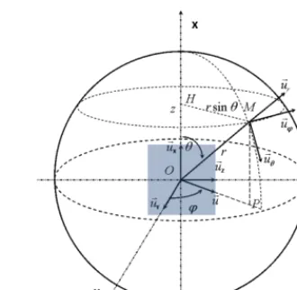
second measurement with the source moved to the right at longitude 𝜑𝜑 = 10° and 𝜃𝜃 = 0° for a total exposure time of 57 h. Count rate is the same. The coordinates system is explained on Figure 6.
Figure 6: Spherical coordinates system - The square represents the detector
From these data, we can build a third augmented data set combining randomly all events from the two independent measurements into a single list.
The count rate being low, (50 counts/s at 30 cm), the chance of spurious double events from the two sources - that we cannot record combining the two event lists - is considered to be negligible (<< 1 count/s). This way, we obtain a representative data set that we would have recorded with two 137Cs sources
simultaneously installed in the field of view the detector. Choosing the number of events in the two lists, allows to virtually modulate the sources relative intensities. It also allows to test our methods with an arbitrary number of sources in the field of view even having only one source available in the lab.
In the results section, we study the Compton reconstruction processed on the measurement with the source at coordinates (10°,0°) and the “augmented data set” with two sources at coordinates (0°,0°) and (10°,0°). Other configurations have been successfully tested with similar performance of the algorithms.
The algorithms are applied with a field of view of 180°×180°. To help the reader to see the results, the images of Figure 7A-D are zoomed in the region of interest, between -30° and 30° for the longitude and between -15° and 15° for the latitude. Based on experience, we apply a discretization of 2°×2° for DBP and Compton inversion, 4°×4° for the Bayesian algorithm and 5°×5° for SOE-RR. We apply a spline interpolation for the representation on the reconstructed image. SOE-RR is performed with 20 000 iterations.
B. Results
The total number of detected events with the acquisition at (10°,0°) is 5 423 829. Applying the energy selection according to the method described in section III, 8119 Compton events are extracted, corresponding to 0.15 % of the total number of recorded events.
With the two sources mix augmented data set, the total number of events is 8 614 247 and 13 076 Compton events are extracted, also corresponding to 0.15 % of the events.
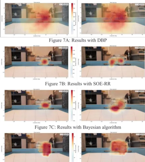
Figure 7A: Results with DBP
Figure 7B: Results with SOE-RR
Figure 7C: Results with Bayesian algorithm
Figure 7D: Results with Compton inversion
Table II: Algorithms performance: computation time, angular resolution FWHM for one source at (10°,0°) and separating power for two sources separated by 10°.
TABLE II
PERFORMANCES OF THE ALGORITHMS
PARAMETER DBP SOE-RR ALGORITHMBAYESIAN INVERSIONCOMPTON
FWHM one source
(10°,0°) 37° 7,9° 8,6° 14,5°
Separation of two
sources (10°) No Yes Yes No
Computation time
(4500 events) 12 s ± 1 s 110 s ± 2 s 12 s ± 1 s
65 s ± 2 s (12 s DBP + 53 s gradient descent) Complexity
according the
number of events Linear Linear Linear
Linear (DBP) + Constant (gradient
descent)
Computation time is evaluated with the following hardware setup: Intel® Xeon® Silver 4114, CPU @ 2,20 GHz. The algorithms are implemented in Python using NumPy library.
C. Comments
The Direct Back-Projection algorithm shows the worst performances in terms of angular resolution. However, it shows the fastest computation time, 12 s to process 4500 events.
SOE-RR shows a way better localization performance, especially with the power to separate two sources 10° apart. However, the main limitation is related to the computation time, nine to ten times slower than DBP. Moreover, as the number of iterations to compute is not pre-determined, the computation time depends on the number of iterations. Nevertheless, this
algorithm considers the uncertainties in the measurement thanks to the Resolution Recovery version, which is important to get a more robust result.
The Bayesian algorithm shows intermediate performances in terms of localization. On Figure 7C right, the left source is not localized at the exact position: this is a discretization effect in the 4°×4° pixelization reconstructed image. In fact, the probability of presence is higher in the neighbouring pixel of the real position of the source. The two sources are however well separated, with a quick computation time similar to the Direct Back-Projection algorithm. Actually, the number of operations is the same as in DBP, since the list of events is scanned only once.
We conclude here that SOE-RR is the most promising algorithm to solve our Compton reconstruction problem with a single layer Compton imager as long as computation time is not an issue. Our Bayesian algorithm gives a fast and relatively accurate result, possibly used in other methods as a better prior than the Direct Back-Projection reconstruction.
Compton inversion algorithm is less convincing than SOE-RR and the Bayesian algorithm for the detection of point sources. However, a preliminary study based on simulations shows that this algorithm will reach better performances in the case of extended sources.
VI. CONCLUSION AND OUTLOOKS
Compton imaging can be performed with a single plane miniature pixelated detector with fine pitch and high energy resolution. It requires a particular attention on the selection of the Compton events, given the configuration and the characteristics of the Caliste-HD detector, followed by a reconstruction algorithm. We tested four algorithms on real data and demonstrated that SOE-RR and a new Bayesian algorithm, are able to separate two sources of 137Cs separated by only10°
which a classical Direct Back Projection cannot do.
D. Compton inversion
The last algorithm we propose is a Compton inversion algorithm of the image initially computed by a Direct Back-Projection method.
A passing matrix 𝑀𝑀 is obtained by simulating the presence of a source in each pixel of the source space image, and applying the DBP to these simulated data, so that we derive, at each possible position in space, the expected DBP pixelated with the same resolution as the source space image.
The line 𝑗𝑗 of 𝑀𝑀 contains the simulated DBP, in flattened data, of a source placed in the pixel 𝑗𝑗 of the source space image.
If we note 𝑌𝑌, the DBP of a real acquisition and 𝑋𝑋, the expected intensities of the source in each pixel of the source space image, the equation to be solved is written as:
𝑌𝑌 = 𝑀𝑀𝑋𝑋 (eq. 11)
𝑀𝑀 is a matrix with high dimensions, of a typical size of 81002
for a field of view of 180°×180° with a discretization of 2°×2°. Its inversion is not feasible; therefore, we may approach an optimal solution of this inverse problem minimizing instead:
𝐿𝐿(𝑋𝑋) = ‖𝑌𝑌 − 𝑀𝑀𝑋𝑋‖�� (eq. 12)
The minimization process is constrained to positive elements of 𝑋𝑋. A gradient descent algorithm computes this minimization, since this is a convex problem.
Once the optimal solution 𝑋𝑋 is found, we apply a TV-regularization [20], which is used in Compton imaging with other algorithms [21], in order to denoise the source space image by minimizing ‖∇𝑋𝑋‖�.
V. TESTS AND PERFORMANCES
A. Test configuration
We take real data with Caliste-HD to apply and test the algorithms. A 1.7 MBq 137Cs source is placed in a distance of
30 cm from the detector at different longitudes and latitudes. The corresponding dose rate is ~1.4 μSv/h at the detector level.
Two separate measurements are acquired: one measurement with a source directly placed on axis, at longitude 𝜑𝜑 = 0° and latitude 𝜃𝜃 = 0° for a total exposure time of 35 h. The corresponding count rate at Caliste level is 50 counts/s/cm2. A
second measurement with the source moved to the right at longitude 𝜑𝜑 = 10° and 𝜃𝜃 = 0° for a total exposure time of 57 h. Count rate is the same. The coordinates system is explained on Figure 6.
Figure 6: Spherical coordinates system - The square represents the detector
From these data, we can build a third augmented data set combining randomly all events from the two independent measurements into a single list.
The count rate being low, (50 counts/s at 30 cm), the chance of spurious double events from the two sources - that we cannot record combining the two event lists - is considered to be negligible (<< 1 count/s). This way, we obtain a representative data set that we would have recorded with two 137Cs sources
simultaneously installed in the field of view the detector. Choosing the number of events in the two lists, allows to virtually modulate the sources relative intensities. It also allows to test our methods with an arbitrary number of sources in the field of view even having only one source available in the lab.
In the results section, we study the Compton reconstruction processed on the measurement with the source at coordinates (10°,0°) and the “augmented data set” with two sources at coordinates (0°,0°) and (10°,0°). Other configurations have been successfully tested with similar performance of the algorithms.
The algorithms are applied with a field of view of 180°×180°. To help the reader to see the results, the images of Figure 7A-D are zoomed in the region of interest, between -30° and 30° for the longitude and between -15° and 15° for the latitude. Based on experience, we apply a discretization of 2°×2° for DBP and Compton inversion, 4°×4° for the Bayesian algorithm and 5°×5° for SOE-RR. We apply a spline interpolation for the representation on the reconstructed image. SOE-RR is performed with 20 000 iterations.
B. Results
The total number of detected events with the acquisition at (10°,0°) is 5 423 829. Applying the energy selection according to the method described in section III, 8119 Compton events are extracted, corresponding to 0.15 % of the total number of recorded events.
With the two sources mix augmented data set, the total number of events is 8 614 247 and 13 076 Compton events are extracted, also corresponding to 0.15 % of the events.
Figure 7A: Results with DBP
Figure 7B: Results with SOE-RR
Figure 7C: Results with Bayesian algorithm
Figure 7D: Results with Compton inversion
Table II: Algorithms performance: computation time, angular resolution FWHM for one source at (10°,0°) and separating power for two sources separated by 10°.
TABLE II
PERFORMANCES OF THE ALGORITHMS
PARAMETER DBP SOE-RR ALGORITHMBAYESIAN INVERSIONCOMPTON
FWHM one source
(10°,0°) 37° 7,9° 8,6° 14,5°
Separation of two
sources (10°) No Yes Yes No
Computation time
(4500 events) 12 s ± 1 s 110 s ± 2 s 12 s ± 1 s
65 s ± 2 s (12 s DBP + 53 s gradient descent) Complexity
according the
number of events Linear Linear Linear
Linear (DBP) + Constant (gradient
descent)
Computation time is evaluated with the following hardware setup: Intel® Xeon® Silver 4114, CPU @ 2,20 GHz. The algorithms are implemented in Python using NumPy library.
C. Comments
The Direct Back-Projection algorithm shows the worst performances in terms of angular resolution. However, it shows the fastest computation time, 12 s to process 4500 events.
SOE-RR shows a way better localization performance, especially with the power to separate two sources 10° apart. However, the main limitation is related to the computation time, nine to ten times slower than DBP. Moreover, as the number of iterations to compute is not pre-determined, the computation time depends on the number of iterations. Nevertheless, this
algorithm considers the uncertainties in the measurement thanks to the Resolution Recovery version, which is important to get a more robust result.
The Bayesian algorithm shows intermediate performances in terms of localization. On Figure 7C right, the left source is not localized at the exact position: this is a discretization effect in the 4°×4° pixelization reconstructed image. In fact, the probability of presence is higher in the neighbouring pixel of the real position of the source. The two sources are however well separated, with a quick computation time similar to the Direct Back-Projection algorithm. Actually, the number of operations is the same as in DBP, since the list of events is scanned only once.
We conclude here that SOE-RR is the most promising algorithm to solve our Compton reconstruction problem with a single layer Compton imager as long as computation time is not an issue. Our Bayesian algorithm gives a fast and relatively accurate result, possibly used in other methods as a better prior than the Direct Back-Projection reconstruction.
Compton inversion algorithm is less convincing than SOE-RR and the Bayesian algorithm for the detection of point sources. However, a preliminary study based on simulations shows that this algorithm will reach better performances in the case of extended sources.
VI. CONCLUSION AND OUTLOOKS
Compton imaging can be performed with a single plane miniature pixelated detector with fine pitch and high energy resolution. It requires a particular attention on the selection of the Compton events, given the configuration and the characteristics of the Caliste-HD detector, followed by a reconstruction algorithm. We tested four algorithms on real data and demonstrated that SOE-RR and a new Bayesian algorithm, are able to separate two sources of 137Cs separated by only10°
which a classical Direct Back Projection cannot do.
VII. REFERENCES
[1] Y.-s. Kim, J. H. Kim, H. S. Lee, H. R. Lee, J. H. Park, J. H. Park, H. Seo, C. Lee, S. H. Park and C. H. Kim, Development of Compton imaging system for nuclear material monitoring at pyroprocessing test-bed facility, 2016: Journal of Nuclear Science and Technology, 53:12, 2040-2048, DOI:.
[2] A. Koide, J. Kataoka, T. Masuda, S. Mochizuki, T. Taya, K. Sueoka, L. Tagawa, K. Fujieda, T. Maruhashi, T. Kurihara and T. Inaniwa, Precision imaging of 4.4 MeV gamma rays using a 3-D position sensitive Compton camera, Scientific Reportsvolume 8, Article number: 8116, 2018.
[3] P. Bloser, R. Andritschke, G. Kanbach, V. Schonfelder, F. Schopper and A. Zoglauer, The MEGA advanced Compton telescope project, New Astronomy Reviews 46 611–616, 2002.
[4] W. Leo, Techniques for Nuclear and Particle Physics Experiments: A How-to Approach, Springer-Verlag, 1993.
[5] S. Takeda, Y. Ichinohe, K. Hagino, H. Odaka, T. Yuasa, S.-n. Ishikawa, T. Fukuyama, S. Saito, T. Sato, G. Sato, S. Watanabe, M. Kokubun and T. Takahashi, Applications and imaging techniques of a Si/CdTe Compton gamma-ray camera, TIPP 2011 - Technology and Instrumentation in Particle Physics 2011. Physics Procedia 37 (2012) 859-866, 2012.
[6] G. Llosa, M. Trovato, J. Barrio, A. Etxebeste, E. Muñoz, C. Lacasta, J. F. Oliver, M. Rafecas, C. Solaz and P. Solevi, First Images of a Three-Layer Compton Telescope Prototype for Treatment Monitoring in Hadron Therapy, Frontiers in Oncology 6:14, 2016. [7] C. Lehner, Z. He and F. Zhang, 4Pi Compton
Imaging Using a 3-D Position-Sensitive CdZnTe Detector Via Weighted List-Mode Maximum Likelihood, IEEE: Transactions on Nuclear Science, Vol. 51, NO. 4, 2004.
[8] O. Limousin, The story of Caliste: CdTe based pixel detectors for Hard X-Ray astronomy in space, Habilitation à Diriger des Recherches, Université Paris-Diderot, CEA, 2016.
[9] A. Andreyev, A. Celler, I. Ozsahin and A. Sitek, Resolution recovery for Compton camera using origin ensemble algorithm, Medical Physics 43, 2016. [10] D. Xu, Z. He, C. E. Lehner and F. Zhang, 4 Pi
Compton imaging with single 3D position sensitive CdZnTe detector, Hard X-Ray and Gamma-Ray Detector Physics VI, Proc. of SPIE Vol. 5540 (SPIE, Bellingham, WA, 2004) · 0277-786X/04/$15 · doi: 10.1117/12.563905, 2004.
[11] A. Meuris, O. Limousin, O. Gevin, F. Lugiez, I. L. Mer, F. Pinsard, M. Donati, C. Blondel, A. Michalowska, E. Delagnes, M.-C. Vassal and F. Soufflet, Caliste HD: a New Fine Pitch Cd(Zn)Te Imaging Spectrometer from 2 ke V up to 1 Me V, 2011:
IEEE Nuclear Science Symposium Conference Record.
[12] S. Dubos, O. Limousin, C. Blondel, R. Chipaux, Y. Dolgorouky, O. Gevin, Y. Ménesguen, A. Meuris, T. Orduna, T. Tourette and A. Sauvageon, Low Energy Characterization of Caliste HD, a Fine Pitch CdTe-Based Imaging Spectrometer, IEEE: Transactions on Nuclear Science, Vol. 60, No. 5, 2013.
[13] A. Michalowska, O. Gevin, O. Lemaire, F. Lugiez, P. Baron, H. Grabas, F. Pinsard, O. Limousin and E. Delages, IDeF-X HD: A low power Multi-Gain CMOS ASIC for the readout of Cd(Zn)Te Detectors, IEEE Nuclear Science Symposuim & Medical Imaging Conference, 2010.
[14] C. E. Ordonez, A. Bolozdynya and W. Chang, Doppler Broadening of Energy Spectra in Compton Cameras, IEEE Nuclear Science Symposium Conference Record, 1998.
[15] A. Meuris, O. Limousin and C.Blondel, Charge sharing in CdTe pixilated detectors, Nuclear Instruments and Methods in Physics Research Section A: Accelerators, Spectrometers, Detectors and Associated Equipment, Volume 610, Issue 1, Pages 294-297, 2009.
[16] G. Daniel, O. Limousin, D. Maier, F. Ceraudo and A. Meuris, Application of Bayesian Convolutional Neural Network to spectral identification of radionuclides for nuclear monitoring, To be submitted TNS 2019, 2019.
[17] D. Maier and O. Limousin, Energy calibration via correlation, Nuclear Instruments and Methods in Physics Research Section A, DOI: 10.1016/j.nima.2015.11.149, 2016.
[18] A. Andreyev, A. Sitek and A. Celler, Fast image reconstruction for Compton camera using stochastic origin ensemble approach, Medical Physics 38, 2010. [19] C. Bobin ; O. Bichler ; V. Lourenço ; C. Thiam ; M.
Thévenin, Applied Radiation and Isotopes, Vol. 109, Pages 405-409, 2015.
[20] A. Chambolle, V. Caselles, M. Novaga, D. Cremers and T. Pock, An introduction to Total Variation for Image Analysis, hal-00437581, 2009.