Article
Refining Land-Cover Classification Maps Based on
Dual-Adaptive Majority Voting Strategy for
Very-High-Resolution Remote Sensing Images
Guo Qing Cui 1,2,5,*, Zhi Yong Lv 3,*, Guang Fei Li 3, Jón Atli Benediktsson 4 and Yu Dong Lu 11 School of Environmental Science and Engineering, Chang’an University, Xi’an 710054, China, [email protected] (G.Q.C); [email protected] (Y.D.L);
2 Key Laboratory of Subsurface Hydrology and Ecological Effects in Arid Region (Chang’an University), Ministry of Education. [email protected] (G.Q.C).
3 School of Computer Science and Engineering, Xi’An University of Technology, Xi’an 710048, China; [email protected] (Z.Y.L.), [email protected] (G.F.L);
4 Faculty of Electrical and Computer Engineering, University of Iceland, Reykjavik IS 107, Iceland; [email protected];
5 The First Topographic Surveying Brigade of Shaanxi Bureau of Surveying and Mapping, Xi’an 710054, China; [email protected](G.Q.C).
* Correspondence: [email protected] (G.Q.C) and [email protected] (Z.Y.L.); Tel.: +86-158-2967-3435
Abstract: Land-cover classification that uses very-high-resolution (VHR) remote sensing images is a topic of considerable interest. Although many classification methods have been developed, there is still room for improvements in the accuracy and usability of classification systems. In this paper, a novel post-processing approach based on a dual-adaptive majority voting strategy (D-AMVS) is proposed for improving the performance of initial classification maps. D-AMVS defines a strategy for refining each label of a classified map that is obtained by different classification methods from the same original image and fusing the different refined classification maps to generate a final classification result. The proposed D-AMVS contains three main blocks. 1) An adaptive region is generated by extending gradually the region around a central pixel based on two predefined parameters (T1 and T2) in order to utilize the spatial feature of ground targets in a VHR image. 2)
For each classified map, the label of the central pixel is refined according to the majority voting rule within the adaptive region. This is defined as adaptive majority voting (AMV). Each initial classified map is refined in this manner pixel by pixel. 3) Finally, the refined classified maps are used to generate a final classification map, and the label of the central pixel in the final classification map is determined by applying AMV again. Each entire classified map is scanned and refined pixel by pixel based on the proposed D-AMVS. The accuracies of the proposed D-AMVS approach are investigated through two remote sensing images with high spatial resolutions of 1.0 and 1.3 m, respectively. Compared with the classical majority voting method and a relatively new post-processing method called general post-classification framework, the proposed D-AMVS can achieve a land-cover classification map with less noise and higher classification accuracies.
Keywords: land-cover classification; very high spatial resolution remote sensing image; adaptive majority vote; post-classification.
1. Introduction
Land-cover classification based on remote sensing images plays an important role in providing information regarding the Earth’s surface [1-4]. For many applications, such as urban vegetation mapping[5], aboveground biomass estimation in forests [6], urban flood mapping[7], and land-use analysis[8], the underlying land-cover information from remote sensing images is necessary.
Very-high-resolution (VHR) remote sensing images are conveniently available and are highly popular in land-cover classification. However, substantial research has demonstrated that salt-and-pepper noise is a common phenomenon in the classification of VHR remote sensing images [9-18].
Some methods have been developed to cope with this problem. For instance, Lv et al. [19] promoted a general post-classification framework for improving land-cover classification, while Huang et al. [20] proposed an SVM ensemble approach for combining different features to improve the classification accuracies of VHR images. In the current study, the methods are grouped into two mainstream techniques. The first relatively popular technique is the spatial–spectral feature-based classification method [14,21,22] where the spatial feature is usually extracted to complement insufficient spectral information. For example, the pixel shape index (PSI) has been used to improve VHR image classification[23]. Zhang et al. extended the PSI from a “pixel” to an “object”1 and
proposed an object-based spatial feature called the object correlative index. Furthermore, various mathematical morphological methods have been developed to describe the structural features and complement the spectral features to improve classification accuracy [22,24-27]. Moreover, spatial filtering is an effective way to reduce noise and extract spatial features. Kang et al. proposed a method based on an edge-preserving filter and image fusion to enhance the classification accuracy[28]. Jia et al. developed an edge-preserving filtering method for improving the performance of VHR image classification [29]. Other methods, such as semantic features[20,30], Markov modeling of spatial features[13], object-based feature extraction[9], and active learning algorithms[31,32], are commonly adopted to complement spectral information for land-cover classification. However, despite various features and techniques promoting VHR image classification, not one method can be labeled as “the best” or “the most appropriate one” for all cases because the classification accuracies for most methods are usually dependent[33,34]. The design and use of feature extraction methods is also very dependent on the case at hand. Therefore, the space for improving the classification accuracy and usability of the VHR image classification method leaves room for improvement.
Post-classification is the second technique in this study. It defines a post-processing strategy often applied to a classified map to remove noise and increase the classification accuracy [35-37]. Several post-classification methods have been proposed. For example, Lu et al. proposed a structural similarity-based label smoothing approach for refining land-cover classification maps[16]. Huang et al. presented a building extraction post-processing framework for VHR imagery. Lv et al. developed a general post-classification framework (GPCF) for improving land-cover mapping by using VHR images[19]. Tang et al. and Huang et al. summarized the post-processing reclassification approaches systematically in their research [35,38]. From their studies, the “sliding window” technique is usually adopted in considering the neighboring information for refining the label of the central pixel, wherein the accuracies of the initial classified maps can be improved. Given that everything is related to everything else, and things that are close are more related than things that are more distant according to Tobler’s first law of geography[39,40], pixels with greater proximity are more likely to belong to the same class in terms of a classification problem by using remote sensing images. However, one limitation in considering contextual information through a regular window is that a regular window shape may not cover the different shapes of ground objects in a particular class (i.e., different shapes of buildings, varying shapes of lakes or meadows, etc.). Therefore, the adaptive ability of considering contextual information in post-classification should be of great interest.
In this study, we extend our previous research on GPCF[19] and propose an approach named dual-adaptive majority voting strategy (D-AMVS). Compared with GPCF, the extension of this study has two aspects. First, in the process of refining the label of an initial classified map, the neighboring information is considered in an adaptive manner through an adaptive irregular region.
Second, when the different classified maps are fused, an optimal selection strategy is proposed to dynamically choose the classified maps according to their local performance in classification. The initial classified maps are first refined based on the adaptive region coupled with the majority voting method. Then, the refined classified maps are taken as a candidate set where the label of each pixel in the final refined classification is determined by the top two refined classified maps, i.e., the maps which present the best performances within the local adaptive region. To demonstrate the effectiveness of this extension, the initial classified maps are obtained by different classifiers or spectral–spatial approaches and compared with the proposed D-AMVS with the existing GPCF and the traditional majority voting approach. Further details will be presented in the following sections.
2. D-AMVS Approach for Refining Initial Classification Maps
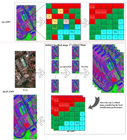
The proposed D-AMVS aims to utilize spatial information in an adaptive manner and fuse multi-source classified maps to reduce the noise of classification maps. Figure 1b shows the main steps of the proposed strategy. 1) The multi-source initial classified maps are acquired by different approaches, such as classifiers or spatial–spectral feature-based approaches. 2) The progress of adaptive majority voting (AMV) is defined in Figure 1a, where AMV is used to refine the initial classified maps; the label of each initial classified map of the pixel is refined with an adaptive region generated by gradually extending the region around a central pixel in the sourcing image. 3) For an adaptive region, the local classification performance of each refined classification map is compared. The top two refined maps are selected, and then the label of the central pixel of the adaptive region is assigned by using the class that appears most frequently. Additional details will be presented in the following paragraphs.
The construction of adaptive region surrounding a pixel is pivotal for the proposed D-AMVS. This study employs an adaptive region around a central pixel that has been proposed in the literature[41]. The shape of an adaptive region represents the contextual features surrounding a
central pixel, and the size of the adaptive region is constrained by two predefined thresholds (T1
and T2) in the spectral and spatial domains. From the investigation in [41], the proposed adaptive
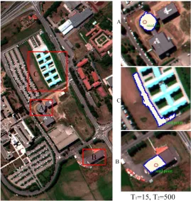
region has an advantage in considering contextual information in an adaptive spatial domain (see [42] for more details). Three examples are given in Figure 2 to show the shape-adaptive ability of the proposed region extension method.
In this study, the adaptive region coupled with the majority voting is used to refine the multi-source initial classification maps. Then, the refined maps are fused to generate a final classification result. An initial multi-source classification map is represented by the set I = {𝐼 , 𝐼 , 𝐼 , ⋯ , 𝐼 }, where N is the total number of initial classified maps. The total number of a specific class (C) within an adaptive region (𝑅 ) can be calculated by Equation (1).
𝑆 = 𝑝 (𝐶 ), 𝑥 ∈ 𝑅 (1)
where 𝑆 is the total number of pixels belonging to the specific class 𝐶 within the adaptive region 𝑅 . Here, 𝑅 is the extended region around the pixel (i,j) in the spatial domain, while
𝑝 (𝐶 ) is labeled as 𝐶 in the initial classified map 𝐼 . In this context, the label of the central pixel xij
can be determined by Equation (2).
C(𝑥 ) = argmax{𝑠 , 𝑠 , 𝑠 , ⋯ 𝑠 } (2)
where M is the total number of the classes for the entire initial classification map; Sm is assumed to be the total number of pixels, which are assigned to the m-th class of the initial classification maps for the adaptive region 𝑅 ; and C(𝑥 ) is the label of the central pixel. Therefore, the label of the
central pixel (𝑥 ) is refined according to the class label, which has the maximum performance in the
set {𝑠 , 𝑠 , 𝑠 , ⋯ 𝑠 }.
An initial classified image can be refined pixel by pixel through the corresponding adaptive region. An example is shown in Figure 1a, where P1, P2, and P3 are the three central pixels, and the
progress is defined as AMV. Compared with the regular window-based majority voting approach, the proposed AMV technique can smoothen the noise of the classification map and preserve the shape of different targets.
Image
…
…
(a) AMV
…
…
Final Classification Map
1 2 2 2 2 2
2 1 3 p1 1 1
3 2 2 1 2 1
0 3 1 4 1 2
1 P2 1 5 1 6
1 1 6 6 P3 6
1 2 6 1 6 1
2 2 2 2 2 2
2 2 2 p1 1 1
2 2 2 1 1 1
2 3 1 1 1 6
1 P2 1 1 1 6
1 1 6 6 P3 6
1 6 6 6 6 6
(b) D-AMV
Initial Classified maps 1st-refined Maps
Overlay
2st-AMV (a)-operation
Select the top-2 refined maps considering the local classification performance
2 2 2 2 2 2
2 2 2 p1 1 1
2 2 2 1 1 1
2 3 1 1 1 6
1 P2 1 1 1 6
1 1 6 6 P3 6
1 6 6 6 6 6
2 2 2 2 2 2
2 2 2 p1 1 1
2 2 2 1 1 1
2 3 1 1 1 6
1 P2 1 1 1 6
1 1 6 6 P3 6
1 6 6 6 6 6
Figure 2. Examples of adaptive regions for the proposed D-AMVS. The green points inside the red circles are the central pixels of each extension, and the blue borders define the shape of the adaptive region.
To further improve the classification accuracy and generate the final classification map, inspired by the previous GPCF[19], the refined classification maps are taken as candidates to obtain
the final classification map. First, the number of classes within an adaptive region (𝑅 ) is counted
and assigned as 𝑁 (𝑅 ), where 𝐼 is the k-th refined classified map. Therefore, the number of classes within an adaptive region can be calculated for each refined map, where the set is assigned
as 𝑁 = {𝑁 𝑅 , 𝑁 𝑅 , 𝑁 𝑅 , ⋯ , 𝑁 (𝑅 )}. Second, the set (𝑁 ) is sorted in descending order.
Then, the top two refined classified maps are taken as the selected maps for the following process. The top two refined classified maps are assigned as 𝐼 and 𝐼 . In theory, because the adaptive region has a relatively greater homogeneity in the spectral domain, the pixels within the adaptive region are usually seen as one target class. Therefore, the less class within an adaptive region means a better classification performance for the local region of a refined map. Finally, the number of pixels in each class from the selected refined classified maps 𝐼 and 𝐼 is considered. The label of the central pixel (i,j) of the adaptive region 𝑅 is refined dually by using the class that appears most frequently in the region. In this context, each pixel of an image is once taken as a central pixel to extend the corresponding adaptive region, and the adaptive region is coupled with the majority voting strategy to select the refined maps and determine the label of each pixel in the final classification map.
classification map by using a regular window and the majority voting technique. On the one hand, because the number of each class within a regular window is affected by the shape of a target when the central pixel of a window is located at the boundary between different classes, determining the label of the central pixel may have a limitation in discrimination. On the other hand, the proposed D-AMVS has the advantage in spatial adaptive ability, wherein the majority voting strategy is applied within an adaptive region that can be adaptive with the shape of a target.
3. Experiment
In this section, two experiments are performed to test the effectiveness of the proposed D-AMVS approach. First, the two images with very high spatial resolutions are described in detail. Then, the experimental design and setting of parameters are presented. Subsequently, the visual performance and quantitative evaluation are shown for comparison.
3.1. Data Set Description
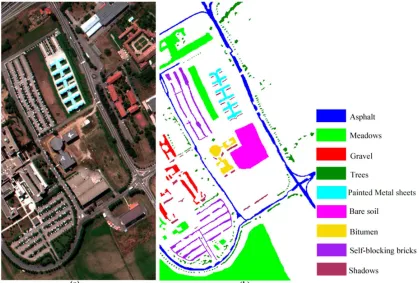
Two data sets are used in the experiments. The first data set is obtained by the Reflective Optics System Imaging Spectrometer (ROSIS-03) sensor on 8 July 2002 [14,42], and the raw data represent the hyperspectral image of a Pavia University scene with 103 bands and 1.0 m/pixel spatial resolution. The location of this data is near Pavia University, which is located north of the city Pavia, Italy. The original data set is 610 × 340 pixels. For the first experiment, Figure 3a shows a false color image composed of channels number 10, 27, and 46 for red, green, and blue, respectively. The ground reference is shown in Figure 3b, where the nine information classes are considered in the experiment, as shown in the legend.
Figure 3. Pavia University image used in the first experiment: (a) false color original image of Pavia University and (b) ground reference data.
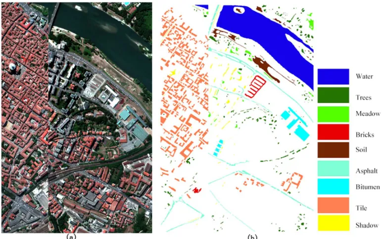
no. 60, 27, and 17 are selected to compose a false color image in red, green, and blue, respectively. Figure 4b illustrates the ground reference and the nine information classes.
Figure 4. Pavia Center image used in the second experiment: (a) false color original image of Pavia Center and (b) ground reference data.
3.2. Experimental Setup and Parameter Setting
In the first experiment, the Pavia University image is adopted to test the effectiveness of the proposed D-AMVS on the basis of the different initial classification maps acquired by different supervised classifiers. A false color image is used as the input data for land-cover classification because the concentration of our study is on VHR remote sensing images. Four classical supervised classifiers are embedded in the business ENVI4.8; specifically, neural net (NN), maximum likelihood classification (MLC), Mahalanobis distance (MD), and support vector machine (SVM) are used to obtain the initial classified maps. The software provided the default parameters of each classifier for the Pavia University image. The details of the training samples and testing pixels are given in Table 1.
Table 1. Number of training samples and reference data for the Pavia University image.
Class Training Samples Test Samples
Asphalt 603 6631
Meadows 396 18649
Gravel 182 2099
Trees 382 3064
Painted metal 46 1345
Bare soil 680 5029
Bitumen 189 1330
Self-blocking bricks 414 3682
Shadows 88 847
Pavia Center scene is adopted for comparison to obtain spatial features. Table 2 shows the number of training and test samples. Based on the above, the parameters of the four spectral–spatial approaches were set to obtain the initial classified maps:
1) Extended morphological profiles (EMPs) [26] are built based on a “disk” structuring element (SE), and the sizes of the SE are equal to 2, 4, 6, and 8 in this experiment.
2) Multi-shape Extended Morphological Profiles (M-EMPs)[25] involves the SE set to shape equaling “disk, square, diamond, line,” and the size of each SE is equal to 8.
3) The parameters of a recursive filter (RF)[28] are set as follows: 𝛿 = 200, 𝛿 = 45.0, and the number of iterations is 3. 𝛿 and 𝛿 denote the spatial and range parameters, respectively. Further details on 𝛿 and 𝛿 can be read in the literature [28].
4) Rolling guidance filter (RGF)[43] is applied to the Pavia Center image with the following parameters: 𝛿 = 200, 𝛿 = 45.0, iteration = 3. In the RGF, 𝛿 and 𝛿 control the spatial range and spatial weights, respectively.
Apart from the above parameter settings for acquiring the initial classified maps in each experiment, the majority voting and the existing GPCF post-classification approaches are applied with a window size from 3 × 3 to 9 × 9, as shown in Tables 4 and 6.
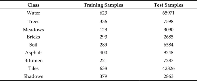
Table 2. Number of training samples and reference data for the Pavia Center image.
Class Training Samples Test Samples
Water 623 65971
Trees 336 7598
Meadows 123 3090
Bricks 293 2685
Soil 289 6584
Asphalt 400 9248
Bitumen 221 7287
Tiles 638 42826
Shadows 379 2863
To guarantee fairness in comparison, the following rules are obeyed in these experiments: 1) The parameters of each approach are acquired through a trial-and-error method. 2) The SVM with an RBF kernel and threefold cross-validation is used as the supervised classifier to classify different spatial–spectral features in the second experiment. 3) The initial classified map with the highest accuracies is selected for post-processing based on majority voting and then compared with GPCF and the proposed D-AMVS.
3.3. Results and Quantitative Evaluation
On the basis of the above experimental setup, the experimental results and comparisons in terms of overall accuracy (OA), Kappa coefficient (Ka), and average accuracies (AA) are detailed below.
been seen that the user’s accuracy of most classes can be improved more or less for the proposed D-AMVs approach.
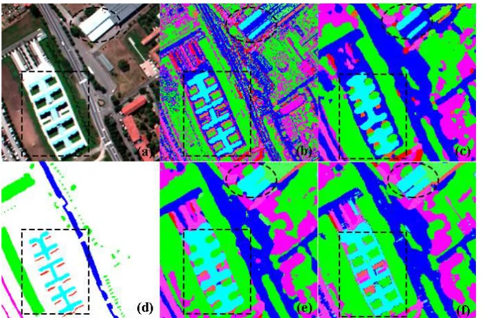
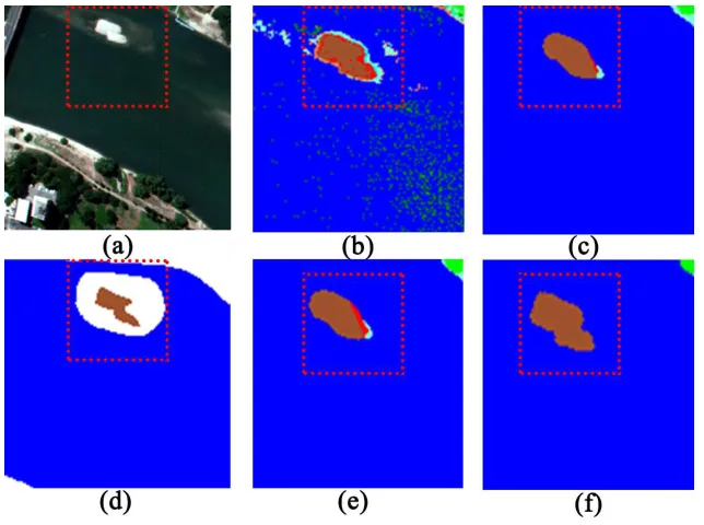
To further demonstrate the advantage of the proposed D-AMVS, Figure 6 shows the zooming in on the observation of comparisons. The observation of the painted metal sheet is represented by the dashed rectangle. The results show the following. First, the shape of the ground target is best preserved in the initial classification map, but much salt-and-pepper noise is observed. Second, although traditional majority voting and GPCF have the ability to remove performance noise, the shape of the ground object cannot be maintained. This situation can be attributed to the regular window, which has a limitation in considering the spatial contextual information, while the shape of the ground target and the window are inconsistent. Compared with the performance of majority voting and GPCF, the proposed D-AMVS achieves the best classification performance and maintains the preferred shape of the ground target. Additional observations can be obtained in the dashed ellipse region of Figure 6.
Table 3. Initial classification results acquired by different classifiers for the Pavia University image.
NN MLC MD SVM
OA(%) 47.21 67.59 53.66 60.92
Ka 0.3824 0.5898 0.4260 0.517
AA(%) 51.58 69.22 56.63 65.39
Table 4. Comparison between the proposed D-AMVS and different post-classification approaches for the Pavia University image.
Majority Voting GPCF Proposed D-AMVS
Window Size 3 5 7 9 3 5 7 9 T1=60, T2=80
OA (%) 73.24 75.68 77.08 78.11 70.25 71.96 72.73 73.2 79.97
Ka 0.659 0.689 0.707 0.72 0.626 0.647 0.657 0.663 0.741
AA (%) 74.63 77.26 78.81 80.08 72.48 75.47 77.38 78.46 81.83
Table 5. Class-specific user’s accuracy (%) in Pavia University image for different methods.
MLC MV
(w = 5 × 5)
GPCF
(w = 5 × 5)
D-AMVs
( T1=60, T2=80)
Asphalt 79.0 86.2 92.9 90.9
Meadows 83.8 86.8 95.0 87.9
Gravel 44.1 64.3 78.0 89.1
Trees 61.0 66.9 52.9 60.2
Painted metal 95.8 96.0 93.5 93.7
Bare soil 33.0 40.7 36.1 51.3
Bitumen 54.5 72.5 67.7 82.9
Self-blocking
bricks 74.2 82.6 73.3 80.5
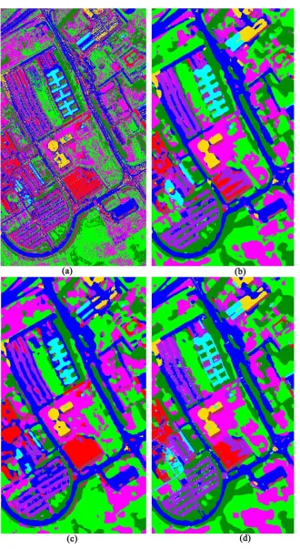
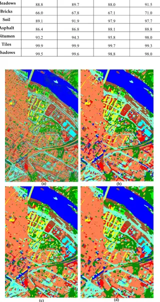
Figure 5. Comparison based on the initial classified maps and different post-classification
approaches for the Pavia University image: (a) initial classification map based on the MLC classifier, (b) post-classification map acquired by GPCF with a 9 × 9 window size, (c) post-classification
map acquired by majority voting with a 9 × 9 window size, and (d) post-classification map
Figure 6. Zoomed comparisons based on the subfigures: (a) Pavia University image, (b) initial classified map obtained by MLC classifier, (c) post-classification map obtained by GPCF with a
9 × 9 window size, (d) ground reference data, (e) post-classification map acquired by majority
voting approach with a 9 × 9 window size, and (f) post-classification map acquired by the
proposed D-AMVS with 𝑇 = 60 and 𝑇 = 80.
Table 6. Initial classified image acquired by different spectral–spatial approaches and the SVM classifier for the Pavia Center image.
EMPs[26] M-EMPs[25] RF[28] RGF[43]
OA (%) 96.04 95.51 93.51 96.72
Ka 0.944 0.937 0.909 0.954
AA (%) 88.82 87.2 82.25 91.06
Table 7. Comparisons between the proposed D-AMVS and different post-classification approaches for the Pavia Center image.
Majority Voting GPCF Proposed D-AMVS
Window Size 3 5 7 9 3 5 7 9 T1=70, T2=80
OA (%) 96.84 96.96 97.02 97.04 97.41 97.46 97.5 97.55 97.66
Ka 0.955 0.957 0.958 0.958 0.963 0.964 0.965 0.965 0.967
AA (%) 91.42 91.81 92.02 92.15 92.47 92.63 92.84 93.09 93.51
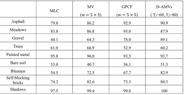
Table 8. Class-specific user’s accuracy in Pavia Center image for different methods.
RGF[43] MV
(w = 5 × 5)
GPCF
(w = 5 × 5)
D-AMVs
( T1=60, T2=80)
Water 99.2 99.1 99.6 99.7
Figure 7. Comparison based on initial classified maps and different post-classification approaches for the Pavia Center image: (a) initial classified map based on RGV spatial–spectral method and SVM classifier, (b) post-classification map acquired by majority voting with a 9 × 9 window size,
Meadows 88.8 89.7 88.0 91.5
Bricks 66.0 67.8 67.1 71.0
Soil 89.1 91.9 97.9 97.7
Asphalt 86.4 86.8 88.1 88.8
Bitumen 93.2 94.3 95.8 98.0
Tiles 99.9 99.9 99.7 99.3
(c) post-classification map acquired by GPCF with a 9 × 9 window size, and (d) post-classification
map acquired by the proposed D-AMVS with 𝑇 = 70 and 𝑇 = 80.
To further investigate the effectiveness and confirm the robustness of the proposed D-AMVS approach, the method is applied to an initial classification map set using the Pavia Center image scene in the second experiment. Tables 6 and 7 show that the proposed D-AMVS achieves higher accuracies than the majority voting and GPCF approaches in each window scale. In addition, the user’s accuracy for each specific class is given in Table 8, and this observation further strength that the proposed D-AMVS approach has the ability in improve the classification accuracy of most classes, such as meadows, bricks, and bitumen. In terms of visual performance and compared with the initial classification map, Figure 7 shows that all the post-classification methods can remove the noise and improve the classification performance. A detailed observation is given through zooming in on the subfigure of the image with the corresponding results shown in Figure 8. From these detailed observations, the proposed D-AMVS has the ability to smooth the noise and maintain the shape of the ground target better.
Figure 8. Zoomed comparisons based on the subfigures: (a) Pavia Center image, (b) initial classified map based on RGV spatial–spectral method and SVM classifier, (c) post-classification map obtained by GPCF with a 9 × 9 window size, (d) ground reference data, (e) post-classification map acquired
by majority voting approach with a 9 × 9 window size, and (f) post-classification map acquired by
the proposed D-AMVS with 𝑇 = 70 and 𝑇 = 80.
4. Discussion
Compared with the traditional majority voting and the previous GPCF[19], both of which are similar to the proposed D-AMVS, the proposed approach can achieve the best accuracies and performance in terms of OA, AA, and Ka. The results shown in Tables 3 to 6 confirm that the proposed D-AMVS can improve the raw accuracies of each initial classification map. To promote the application of the proposed approach, the sensitivity of the parameters is discussed in this section.
The sensitivity between the parameter settings and the classification accuracies for the Pavia University Image in the first experiment is examined. The proposed D-AVMS approach contains two parameters, T1 and T2, for refining and fusing the initial classification maps. As shown in Figure
9a for the first experiment, when T1 is increased from 5 to 35 with the T2 = 100, the OA and AA
and T1 is smaller, an adaptive region around a pixel is generated. This phenomenon happens
because when T1 is small, the spatial information cannot be considered sufficient for refining the
classification map and smoothing the noise. With the increase of T1, more spatial information can be
utilized to smoothen the noise and improve the classification accuracies. Nonetheless, when the accuracies of OA and AA reach the maximum level, the accuracies remain nearly at the same levels with an increase in T1. On the contrary, when T1 is fixed at 60 and T2 is varied from 10 to 150, a
similar conclusion can be acquired as shown in Figure 9b. Furthermore, Figure 9c shows that when
the value of T1 ranges from 5 to 35, the Ka slowly escalates to the maximum value and remains at a
similar level with the increase of T1. This test indicates that T1 is a parameter representing the
spectral difference between the central pixel and its surround pixels, and T2 is the total number of
pixels within the extended adaptive region. T1 and T2 are complementary to one another in the
application of D-AMVS.
Figure 9. Relationship between classification maps and parameter settings (T1 and T2) of the proposed D-AMVS method: (a), (b), and (c) are the relationships between T1, T2, and OA/AA/Ka, respectively, for the Pavia University image; (d), (e), and (f) present the relationships between T1, T2, and OA/AA/Ka for the Pavia Center image, respectively.
Figure 9d illustrates the sensitivity between T1 and the classification accuracies with T2 = 100 in
the second experiment, which uses the Pavia Center image. The sensitivity result clearly indicates
that OA and AA increase gradually when the value of T1 ranges from 5 to 40. However, OA and AA
remain at similar levels when the value of T1 is larger than 40. In addition, when T1 is fixed at 70
and T2 varies from 10 to 150 (Figure 9e), OA and AA post trends similar to those of T2 versus OA
and AA.
From the view of theory, despite the capability of the proposed D-AMV post-processing to reduce the noise of a classification map, it still has the risk of excessive smoothing in the boundary between different classes or of changing the shape of a target. Therefore, a suitable balance between smoothing the noise of classification maps and preserving the details of different classes should be considered in the practical application of the proposed D-AMV approach.
Based on the above discussion for the two experiments, (1) different data may have varying optimal settings of parameters for T1 and T2, where the settings of T1 and T2 should be adjusted
varies. The practice of setting the parameters is beneficial when the proposed D-AMVS approach is applied.
5. Conclusions
In this paper, we extend our previous research on GPCF to the D-AMVS to refine initial classification maps. In the proposed D-AMVS, adaptive regions extend gradually from a central pixel to a pixel group that has spectral similarity and is spatially contiguous to utilize the spatial contextual information in an adaptive manner. Then, the extended adaptive region is coupled with the majority voting to refine the label of the central pixel for an initial classified map in the process defined as AMV. Each initial classified map is scanned and processed in this manner to generate the refined candidate’s maps. Finally, the top two refined classification maps are selected by comparing their classification performance within their adaptive regions. The two selected refined maps are then used to determine the label of the central pixel in the final classification map by again using the AMV. The contribution of this study can be summarized as follows:
(1) The proposed D-AMVS provides competitive accuracies in land-cover classification of VHR
remote sensing images. The two image scenes located in urban areas with various ground targets and different shapes are employed to investigate the performance and effectiveness of the proposed D-AMVS approach. The classification results based on the two image scenes demonstrate the effectiveness and superiority of the proposed approach in terms of visual performance and quantitative accuracies compared with the traditional majority voting and the previous GPCF[19] post-classification approaches.
(2) To the best of our knowledge, this study is the first to promote the idea of D-AMVS for
refining the initial classified map and improving the performance of land-cover classification. Experimental results demonstrate that the proposed approach can preserve the shape and boundary of ground targets because the pixels are highly correlated with their neighbors in the image spatial domain, especially for a ground target (such as a meadow). This correlation is consistent with the shape and size of the target. In the proposed D-AMVS, the neighboring information around a central pixel is utilized through an adaptive region that is constructed by gradually detecting the spectral similarity between the central pixel and its neighbors. Thus, the pixels within an adaptive region are homogeneous in the spectral domain and contiguous in the spatial domain. Moreover, applying the proposed adaptive region to refine the label of an initial classified map is objective and reasonable.
Although the proposed D-AMVs have several advantages, it still has some limitations, such as 1) the time-consuming and experience-dependent process of determining T1 and T2 and 2) an
unreasonable adaptive region will be caused when a mixed pixel is taken as the seed-pixel for an extension. Therefore, in future studies, additional investigations based on different remote sensing images with very high spatial resolution will be conducted to enhance the robustness of the proposed approach. During the experimental section, the determination of optimal compositions for T1 and T2 is time consuming. Thus, the automation of parameter settings for T1 and T2 should be
considered in future studies.
Acknowledgment: The National Science Foundation China (61701396), the Natural Science Foundation of Shaan Xi Province (2017JQ4006), and the project from the China Postdoctoral Science Foundation (2015M572658XB) supported this study.
Author Contributions: Guo Qing Cui and Zhi Yong Lv contributed equally to this study and are responsible for the original idea and experimental design. Guang Fei Li conducted the experiments and provided several helpful suggestions. Jón Atli Benediktsson provided ideas to improve the quality of the study. Yu Dong Lu provided numerous comments for the improvement and revision of this paper.
References
1. Anderson, J.R. A land use and land cover classification system for use with remote sensor data. US Government Printing Office: 1976; Vol. 964.
2. Hansen, M.C.; DeFries, R.S.; Townshend, J.R.; Sohlberg, R. Global land cover classification
at 1 km spatial resolution using a classification tree approach. International journal of remote sensing 2000, 21, 1331-1364.
3. Stefanov, W.L.; Ramsey, M.S.; Christensen, P.R. Monitoring urban land cover change: An
expert system approach to land cover classification of semiarid to arid urban centers.
Remote sensing of Environment 2001, 77, 173-185.
4. Tucker, C.J.; Townshend, J.R.; Goff, T.E. African land-cover classification using satellite
data. Science 1985, 227, 369-375.
5. Feng, Q.; Liu, J.; Gong, J. Uav remote sensing for urban vegetation mapping using random
forest and texture analysis. Remote Sensing 2015, 7, 1074-1094.
6. Lu, D.; Chen, Q.; Wang, G.; Liu, L.; Li, G.; Moran, E. A survey of remote sensing-based
aboveground biomass estimation methods in forest ecosystems. International Journal of
Digital Earth 2016, 9, 63-105.
7. Joyce, K.E.; Belliss, S.E.; Samsonov, S.V.; McNeill, S.J.; Glassey, P.J. A review of the status of satellite remote sensing and image processing techniques for mapping natural hazards and disasters. Progress in Physical Geography 2009, 33, 183-207.
8. Cheng, G.; Han, J.; Guo, L.; Liu, Z.; Bu, S.; Ren, J. Effective and efficient midlevel visual
elements-oriented land-use classification using vhr remote sensing images. IEEE
Transactions on Geoscience and Remote Sensing 2015, 53, 4238-4249.
9. Blaschke, T. Object based image analysis for remote sensing. ISPRS journal of
photogrammetry and remote sensing 2010, 65, 2-16.
10. Li, M.; Zang, S.; Zhang, B.; Li, S.; Wu, C. A review of remote sensing image classification
techniques: The role of spatio-contextual information. European Journal of Remote Sensing 2014, 47, 389-411.
11. Hu, F.; Xia, G.-S.; Hu, J.; Zhang, L. Transferring deep convolutional neural networks for the
scene classification of high-resolution remote sensing imagery. Remote Sensing 2015, 7, 14680-14707.
12. Myint, S.W.; Gober, P.; Brazel, A.; Grossman-Clarke, S.; Weng, Q. Per-pixel vs. Object-based
classification of urban land cover extraction using high spatial resolution imagery. Remote Sensing of Environment 2011, 115, 1145-1161.
13. Moser, G.; Serpico, S.B.; Benediktsson, J.A. Land-cover mapping by markov modeling of
spatial–contextual information in very-high-resolution remote sensing images. Proceedings
of the IEEE 2013, 101, 631-651.
14. Fauvel, M.; Tarabalka, Y.; Benediktsson, J.A.; Chanussot, J.; Tilton, J.C. Advances in
15. Luo, F.; Du, B.; Zhang, L.; Zhang, L.; Tao, D. Feature learning using spatial-spectral
hypergraph discriminant analysis for hyperspectral image. IEEE Transactions on Cybernetics
2018.
16. Lu, Q.; Huang, X.; Liu, T.; Zhang, L. A structural similarity-based label-smoothing
algorithm for the post-processing of land-cover classification. Remote Sensing Letters 2016, 7, 437-445.
17. Huang, X.; Lu, Q. In A novel relearning approach for remote sensing image classification post-processing, Geoscience and Remote Sensing Symposium (IGARSS), 2014 IEEE International, 2014; IEEE: pp 3554-3557.
18. Blaschke, T.; Hay, G.J.; Kelly, M.; Lang, S.; Hofmann, P.; Addink, E.; Feitosa, R.Q.; van der
Meer, F.; van der Werff, H.; van Coillie, F. Geographic object-based image analysis–towards a new paradigm. ISPRS journal of photogrammetry and remote sensing 2014, 87, 180-191.
19. Lv, Z.; Zhang, X.; Benediktsson, J.A. Developing a general post-classification framework for
land-cover mapping improvement using high-spatial-resolution remote sensing imagery.
Remote Sensing Letters 2017, 8, 607-616.
20. Huang, X.; Zhang, L. An svm ensemble approach combining spectral, structural, and
semantic features for the classification of high-resolution remotely sensed imagery. IEEE Transactions on Geoscience and Remote Sensing 2013, 51, 257-272.
21. Bruzzone, L.; Carlin, L. A multilevel context-based system for classification of very high
spatial resolution images. IEEE Transactions on Geoscience and Remote Sensing 2006, 44, 2587-2600.
22. Ghamisi, P.; Dalla Mura, M.; Benediktsson, J.A. A survey on spectral–spatial classification
techniques based on attribute profiles. IEEE Transactions on Geoscience and Remote Sensing 2015, 53, 2335-2353.
23. Zhang, L.; Huang, X.; Huang, B.; Li, P. A pixel shape index coupled with spectral
information for classification of high spatial resolution remotely sensed imagery. IEEE Transactions on Geoscience and Remote Sensing 2006, 44, 2950-2961.
24. Song, B.; Li, J.; Dalla Mura, M.; Li, P.; Plaza, A.; Bioucas-Dias, J.M.; Benediktsson, J.A.; Chanussot, J. Remotely sensed image classification using sparse representations of morphological attribute profiles. IEEE Transactions on Geoscience and Remote Sensing 2014,
52, 5122-5136.
25. Lv, Z.Y.; Zhang, P.; Benediktsson, J.A.; Shi, W.Z. Morphological profiles based on
differently shaped structuring elements for classification of images with very high spatial resolution. IEEE Journal of Selected Topics in Applied Earth Observations and Remote Sensing 2014, 7, 4644-4652.
26. Benediktsson, J.A.; Palmason, J.A.; Sveinsson, J.R. Classification of hyperspectral data from
urban areas based on extended morphological profiles. IEEE Transactions on Geoscience and
Remote Sensing 2005, 43, 480-491.
27. Dalla Mura, M.; Benediktsson, J.A.; Waske, B.; Bruzzone, L. Morphological attribute profiles
28. Kang, X.; Li, S.; Benediktsson, J.A. Feature extraction of hyperspectral images with image fusion and recursive filtering. IEEE Transactions on Geoscience and Remote Sensing 2014, 52, 3742-3752.
29. Xia, J.; Bombrun, L.; Adali, T.; Berthoumieu, Y.; Germain, C. In Classification of hyperspectral data with ensemble of subspace ica and edge-preserving filtering, Acoustics, Speech and Signal Processing (ICASSP), 2016 IEEE International Conference on, 2016; IEEE: pp 1422-1426.
30. Sun, H.; Sun, X.; Wang, H.; Li, Y.; Li, X. Automatic target detection in high-resolution
remote sensing images using spatial sparse coding bag-of-words model. IEEE Geoscience
and Remote Sensing Letters 2012, 9, 109-113.
31. Tuia, D.; Volpi, M.; Copa, L.; Kanevski, M.; Munoz-Mari, J. A survey of active learning
algorithms for supervised remote sensing image classification. IEEE Journal of Selected Topics in Signal Processing 2011, 5, 606-617.
32. Huang, X.; Lu, Q.; Zhang, L. A multi-index learning approach for classification of
high-resolution remotely sensed images over urban areas. ISPRS journal of photogrammetry
and remote sensing 2014, 90, 36-48.
33. Wilkinson, G.G. Results and implications of a study of fifteen years of satellite image
classification experiments. IEEE Transactions on Geoscience and Remote Sensing 2005, 43, 433-440.
34. Liu, D.; Xia, F. Assessing object-based classification: Advantages and limitations. Remote
Sensing Letters 2010, 1, 187-194.
35. Tang, Y.; Atkinson, P.M.; Wardrop, N.A.; Zhang, J. Multiple-point geostatistical simulation
for post-processing a remotely sensed land cover classification. Spatial Statistics 2013, 5, 69-84.
36. Su, T.-C. A filter-based post-processing technique for improving homogeneity of pixel-wise
classification data. European Journal of Remote Sensing 2016, 49, 531-552.
37. Tu, Z.; Van Der Aa, N.; Van Gemeren, C.; Veltkamp, R.C. A combined post-filtering
method to improve accuracy of variational optical flow estimation. Pattern Recognition 2014,
47, 1926-1940.
38. Huang, X.; Lu, Q.; Zhang, L.; Plaza, A. New postprocessing methods for remote sensing
image classification: A systematic study. IEEE Transactions on Geoscience and Remote Sensing 2014, 52, 7140-7159.
39. Tobler, W.R. A computer movie simulating urban growth in the detroit region. Economic
geography 1970, 46, 234-240.
40. Lv, Z.; Zhang, P.; Atli Benediktsson, J. Automatic object-oriented, spectral-spatial feature
extraction driven by tobler’s first law of geography for very high resolution aerial imagery classification. Remote Sensing 2017, 9, 285.
41. ZhiYong, L.; Shi, W.; Benediktsson, J.A.; Gao, L. A modified mean filter for improving the
42. Kunkel, B.; Blechinger, F.; Lutz, R.; Doerffer, R.; van der Piepen, H.; Schroder, M. In Rosis (reflective optics system imaging spectrometer)-a candidate instrument for polar platform missions, Optoelectronic technologies for remote sensing from space, 1988; International Society for Optics and Photonics: pp 134-142.