Article
1
Climate change impacts assessment in coastal
2
lagoons using available modelling tools
3
Bruno Primo 1,2*, Fernanda Achete1,2, Sarith Mahanama3, Marcus Thatcher4, Mark Hemer5,
4
Sutat Weesakul6 and Trang Duong7
5
1 Universidade Federal do Rio de Janeiro (UFRJ), Rio de Janeiro, RJ, Brazil
6
2 Vortex Mundus, Rio de Janeiro, RJ, Brazil
7
3 Global Modeling and Assimilation Office, NASA, Goddard Space Flight Center, Greenbelt, Maryland, USA
8
4 CSIRO Oceans & Atmosphere, Private Bag 1, Aspendale VIC 3195, Australia
9
5 CSIRO Oceans & Atmosphere, GPO Box 1538, Hobart TAS 7001 Australia
10
6 Asian Institute of Technology, Bangkok, Thailand, Hydro and Agro Informatics Institute, Bangkok,
11
Thailand
12
7 IHE Delft and Deltares
13
* Correspondence: brunovps@gmail.com; Tel.: +55-21-98828-0606
14
15
Abstract: Climate change such as sea level rise, change in temperature, precipitation, and storminess
16
are expected to impact significantly coastal lagoons. The nature and magnitude of these impacts are
17
uncertain. The objective of the research is to determine the climate change impacts on mixing and
18
circulation at Songkhla lagoon, Thailand. Songkhla lagoon is the largest lagoonal water resource in
19
Thailand and Southeast Asia. The lagoon is a combined freshwater and estuarine complex of high
20
productivity which represents an extraordinary combination of environmental resources believed
21
to be unique in the region.
22
This work is part of a Climate Change impact assessment framework. It is the validation phase (step
23
5) of the framework applying a case study. Delft 3D was used to simulate CC scenarios in the climate
24
downscaling models, part of the previous framework steps. These results were compared to the
25
current conditions to determine the main changes in mixing and circulation in the coastal lagoon.
26
Three indicators were applied to quantify the impacts: flushing time, salinity intrusion and
27
stratification.
28
The results suggest an increase in water velocities at the inlet in future scenarios and a decrease of
29
flushing time. Salinity and stratification showed more complex changes in futures scenarios.
30
Keywords: water quality; hydrodynamics; flushing time; residence time; downscaling; stratification
31
32
1. Introduction
33
A coastal lagoon is a shallow water body separated from the ocean by a barrier, connected at least
34
intermittently to the ocean by one or more restricted inlets [1,2]. They account for thirteen percent of
35
all coastal environments and usually are poorly flushed and exhibit long resident times [3,4]. Coastal
36
lagoons support a range of natural services that are highly valued by society, including but not
37
limited to fisheries, storm protection, and tourism. They are highly productive ecosystems and
38
support a variety of habitats including salt marshes, seagrasses, and mangroves. They also provide
39
essential habitat for many fish and shellfish species [5].
40
41
Coastal lagoons are ephemeral on a geologic time scale and were formed by a combination of
sea-42
level variation and longshore drift [2,5]. Near the end of Pleistocene (15,000 years ago), the mean sea
43
level rose 130m flooding river valleys and low-lying coastal depressions. Sediment transport can
44
reshape the coast by growing spits and barriers islands forming coastal lagoons [6]. These lagoons
45
can also be formed in marginal depressions behind barriers of active river delta systems [7]. Once
46
formed, they are subject to rapid sedimentation and will eventually change into other types of
47
environments through sediment infilling, tectonic activity, eustatic change in sea level, and land-use
48
activities. Geologically, this change is rapid and can be expected to occur within decades to centuries
49
[6].
50
The size of coastal lagoons varies substantially, ranging in area from less than 0.01km2 to more than
51
10,000 km2, as in the case of Lagoa dos Patos – Brazil. The average depth varies from 1 to 3 m and
52
rarely is exceed 5m, except for the inlet and other tidal channels. Depending on local climatic
53
conditions, salinity can vary from completely fresh to hypersaline [2].
54
Coastal lagoons experience the same forcing as coastal estuaries: river inflow, wind stress, tides,
55
precipitation-evaporation balance, and surface heat balance. However, they respond unequally to
56
these forcing because of differences in geomorphology. The lagoon circulation determines the water
57
and salt balance, water quality, eutrophication, turnover, residence and flushing times [2].
58
Hydrodynamics and water renovation are of prime importance for planning and implementation of
59
coastal management strategies in coastal lagoons [6]. Although circulation, mixing and exchange
60
have been studied extensively in coastal plain estuaries, these processes have been less synthesized
61
for coastal lagoons.
62
1.1 CC impacts on coastal lagoons
63
Climate change is expected to impact sea level rise (SLR), temperature, precipitation, and
64
storminess; therefore, severe changes are expected to occur in coastal lagoons [5,8]. In this study the
65
impacts of sea level rise and precipitation were investigated.
66
67
1.1.1 Sea Level Rise (SLR)
68
Due to glacial melting and thermal expansion of the oceans, mean sea level, on a global scale,
69
has been increasing over the past century and is expected to keep increasing in the future. IPCC (2007)
70
estimated an increase between 0.18 and 0.79 (including an allowance of 0.2m for the uncertainty
71
related to Ice sheet flow) by the end of 21st century.
72
The rapid change in sea level can profoundly alter estuarine ecosystem worldwide. The most
73
affected are the low-lying estuaries where the higher sea levels increase the salt water exchange rate
74
increasing salinity inside the estuary. Higher salt concentration impacts the system ecology as well
75
as circulation due to baroclinic processes [8].
76
SLR leads to increase of overall estuarine depth. Light attenuation is directly proportional to
77
local depth, therefore deeper estuaries decrease primary production and impacting the entire food
78
web. It increases the chances of anoxic sediment changing geochemical processes and enhance
79
stratification, since it requires higher wind stresses to mix the deeper water column [8,5].
80
1.1.2 Precipitation
81
Global Climate Change will modify the precipitation regime intensity, timing, volume and
82
distribution. Superficial runoff is dependent on the precipitation and soil cover, so the increase in
83
precipitation may increase delivery of nutrients. At the same time the changes in runoff can impact
84
the lagoon flushing time.
85
Change in precipitation affects salinity in estuaries, the increase of freshwater runoff decrease
86
salinity on contrary the decrease in precipitation increase estuarine salinity. Modification in salinity
87
1.2 Climate Change Impact Assessment Framework
89
Numerical models are widely applied tool to investigate the possible impacts of the
90
aforementioned forcing changes would have on coastal lagoon. Climate change impacts investigation
91
would require a simulation for the entire period of interest, typically 50-100 years. However,
92
simulations for more than 5 years, even with reduced and schematized forcing conditions have been
93
unsuccessful [9]. A number of studies have been attempted using different approaches to perform
94
long period simulations [10-13] but have been only partially successful. The main problem of these
95
approaches is the accumulation of numerical errors in the computational domain.
96
A model capable of producing reliable 50-100 year predictions with concurrent water level, wave
97
and river flow forcing does not currently exist. Even if such model was available, the high
98
computational demand of the model would limit the number of scenarios and reduce the capacity to
99
simulate the large uncertainty inherent to climate change impact studies. Climate change impact
100
assessment contain many uncertainties. In order to reduce these uncertainties, a train of numerical
101
models could be used. [14] present an ensemble modeling framework that could be used for robust
102
assessment climate change impacts (Figure 1). This approach shows the model development from a
103
global scale to a local site scale via a logical sequencing. The last step (Step 5) of the approach is
104
related to the use of an appropriate coastal impact model for investigating the system diagnostic.
105
Figure 1: Suggested standard modelling framework for a climate change impact quantification study
107
on sandy coasts [from: 15].
108
This work is embedded in this framework as an application of step 5. The aim of this paper is to
109
measure the potential impact of CC in mixing and circulation of coastal lagoons using three different
110
indicators flushing time, salinity and stratification. Songkhla lagoon, Thailand is used as study case.
111
This study is part of a project called “Climate Change Impacts on Small Tidal Inlets (CC-STI)” lead
112
by UNESCO-IHE. The main objective of CC-STI is to determine how the climate change will impact
113
on STIs and what are the best adaptation strategies.
114
We perform short simulations considering future climate change scenarios, derived from the
115
previous framework steps. A process-based model is calibrated and validated for the present
116
conditions then simulated for a period of one year using possible future forcing (e.g. 2050, 2100).
117
2. Materials and Methods
118
In this session we briefly describe the models and steps followed to apply the CC assessment
119
framework until the step 5, the focus of this work.
120
2.1 CC framework Model Description
121
2.1.1 Atmospheric Model
122
The atmospheric model used as step 1 in this study was the Conformal Cubic Atmospheric
123
Model (CCAM). The CCAM is designed as a semi-implicit, semi-Lagrangian atmospheric climate
124
model based on a conformal cubic grid [16,17]. A variable resolution grid was used by applying
125
Schmidt transformation [18], which results in a finer grid resolution over the target area at the
126
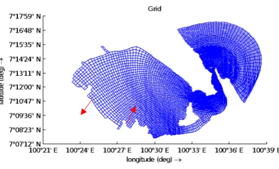
expense of a coarser resolution on the opposite side of the globe (Figure 2).
127
128
129
Figure 2: Plot of the variable resolution conformal cubic grid used for the finer resolution simulations
130
The CCAM physical parameterizations used for this paper include a prognostic cloud scheme
132
[19] and convection based on the approach by [20]. The land-surface scheme supports 6 levels of soil
133
temperature and moisture as well as up to three levels of snow [21]. For these experiments a stability
134
dependent boundary layer scheme was used [22] with non-local vertical mixing following [23], and
135
enhanced mixing of cloudy boundary layer air [24]. Gravity wave drag is parameterized following
136
[25]. Short wave and Long wave radiation for these experiments was parameterized according to
137
[26,27], respectively. Eighteen vertical levels were from 40m to 35km.
138
Step 2 accounts for uncertainty, Sea Surface Temperatures are taken from six CMIP3 General
139
Circulation Models (GCMs) to provide a surface boundary condition for ocean grid points. Monthly
140
biases in the GCM SST datasets were estimated from the 20C3M experiment (1971-2000) after
141
comparing with Reynolds SST climatology. The monthly biases where then subtracted from the
142
GCM SSTs for each simulation month, including the future climate. This provided a ‘bias corrected’
143
SST dataset. Once the bias corrected GCM SST datasets are generated, CCAM is run without
144
atmospheric nudging to create an atmospheric dataset which is consistent with the changes to the
145
SSTs.
146
Two of the better performing 65 km resolution host simulations (i.e., SSTs from GFDL2.1 and
147
ECHAM5 GCMs) were selected to further downscale to approximately 15 km resolution over
148
Thailand, step 3. The 15 km resolution experiments used a C48 grid (i.e., 48 x 48 grid points in the
149
horizontal for each of the six cubic panels). To compensate for errors arising from the coarse
150
resolution region on the opposite side of the globe to the target region, we use a scale-selective filter
151
[28], which perturbs the simulated atmosphere towards the host 65 km resolution simulation at
152
length scales greater than 700 km in diameter. In this way, large scale atmospheric circulation is
153
assimilated from the host 65 km resolution simulation, whereas finer scale atmospheric behavior is
154
simulated by the nested simulation. This approach ensures a high degree of consistency between
155
the host and regional model.
156
2.1.2 Hydrological Model
157
In step 4, the hydrologic model used in this study is the Catchment Land Surface Model (CLSM:
158
[29,30]). CLSM is a macroscale hydrologic model that balances both surface water and energy at the
159
Earth’s land surface. The controls of vegetation on land–atmosphere moisture and energy fluxes
160
within CLSM can be considered to constitute a soil–vegetation–atmosphere transfer scheme (SVAT).
161
One distinguishing characteristic of CLSM is that it considers irregularly shaped, topographically
162
delineated, hydrologic catchment as the fundamental element on the land surface for computing land
163
surface processes. Each catchment is further partitioned into three regimes: 1) a saturated region,
164
from which evaporation occurs with no water stress and over which rainfall is immediately converted
165
to surface runoff, 2) a sub-saturated region, from which transpiration occurs with no water stress and
166
over which rainwater infiltrates the soil, and 3) a ‘‘wilting’’ region, in which transpiration is shut off.
167
The relative areas of these regions vary dynamically; they are unique functions of the Catchment
168
LSM’s three water prognostic variables and the topographic characteristics of the catchment. By
169
continually partitioning the catchment into hydrologically distinct regimes and then applying
170
different regime-appropriate physics within each regime, the Catchment LSM should, at least in
171
principle, provide a more realistic representation of surface energy and water processes. Thus, in
172
contrast with most SVATs, the CLSM accounts for the spatial heterogeneity in soil moisture
173
characteristics within computational elements. In Sri Lanka the model reproduced observed
174
streamflow with a greater degree of accuracy and they extended their study to investigate the impact
175
of soil moisture initial conditions to seasonal streamflow predictability [31].
176
2.1.3 Meteorological Forcing
177
A suite of widely used Atmosphere Ocean General Circulation Models (AOGCMs) produced
178
climate simulations for various carbon dioxide emission scenarios for the Intergovernmental Panel
179
on Climate Change Fourth Assessment Report (IPCC AR4). Climate simulations from two AOGCMs
180
climate change impact analyses. SRES A2 is characterized by heterogeneous world with increasing
182
global population and regional economic growth. The CSIRO CCAM Regional Climate Model
183
dynamically downscaled ECHAM and GFDL climate simulations and provided surface
184
meteorological forcings for the study. The provided 6-hourly, 0.5-degree, surface meteorological
185
forcings included shortwave radiation, longwave radiation, total precipitation, convective
186
precipitation, surface pressure, air temperature at 2m, specific humidity at 2m, and wind for 3
187
different periods: i) hindcast, climate simulations for the period 1981-2000; ii) climate projections for
188
the period 2041-2060, and iii) climate projections for the period 2081-2100. The Catchment Land
189
Surface Model was forced in offline mode using downscaled surface meteorological forcings to
190
generate streamflow at river mouths in study lagoons.
191
2.1.3 Coastal Model
192
The step 5 is the validation of the framework in a local scale. The coastal model used for this step
193
was Delft3D. Delft3D-FLOW is a multi-dimensional (2D or 3D) hydrodynamic and transport
194
modeling system of Deltares for the aquatic environment which calculates non-steady flow and
195
transport phenomena that result from tidal and meteorological forcing on a rectilinear or a
196
curvilinear, boundary fitted grid [32]. The differential equations solved numerically in the model are:
197
the horizontal momentum equations, the continuity equation, the transport equation, and a
198
turbulence closure model. Vertical accelerations are assumed to be small so the vertical momentum
199
equation is reduced to the hydrostatic pressure relation. In 3D simulations, the vertical grid is defined
200
following the sigma co-ordinate approach.
201
Delft3D-WAQ is a 3-dimensional water quality model that solves the
advection-diffusion-202
reaction equation and allows great flexibility in the substances to be modeled. It should be coupled
203
to Delft3D-FLOW or another model to get hydrodynamic conditions.
204
2.2 Study Area
205
Songkhla lagoon is the largest lagoonal water resource in Thailand and Southeast Asia and is
206
made up of three interconnected lakes (Figure 3). Southern Songkhla Lake, known as Thale Sap
207
Songkhla, is the outer lagoon of the system and discharges into the Gulf of Thailand through a small
208
channel which also serves as the harbor entrance to the town of Songkhla. The depth of the harbor
209
and its channel are maintained at six to eight meters. An open lagoon with an undisturbed circulation
210
of fresh and brackish water is a prerequisite for a stable and healthy ecosystem. Any change in this
211
213
214
Figure 3: Location Map of Songkhla Lagoon
215
Around 21 years of hourly water level data is available for two points: Songkhla and Pattani.
216
These data were used as calibration of the numerical model. The maximum tidal range is about 0.7m
217
for Pattani and 0.6 for Songkhla during spring tides
218
Velocity data was digitalized from [33]. Current measurements of two points were conducted
219
during the dry season during 6 days of 1997. The points are located in the two channels formed by
220
the island, one at the north and one at the south of the Ko Yo island. The observed tidal current
221
fluctuation north of Ko Yo Island in June 1997, shows a maximum current speed of about 0.4 m/s
222
during flood tide (Figure 6). South of Ko Yo the maximum registered was about 0.3 m/s.
223
Salinity data was digitalized from [34]. The point is located very close to the island in a very
224
shallow area and the measurement was conducted during October of 2006.The observed salinity
225
fluctuation at point A, shows a maximum salinity of about 32.4 psu and a minimum of about 31.
226
The curvilinear model grid was constructed in a spherical coordinate system with the total of
227
10159 grid cells using the Delft3D-RGFGRID. The grid size varies in space such that finer grids are
228
located in the inlet (20x30 m) and coarser (370x420 m) grids are located in the northern part of the
229
lake (Figure 4) 10 vertical layers were used.
230
The bathymetry inside the lagoon has an average depth of 1.5m. Most of the lagoon has a depth
231
around 2m, in the channel entrance the depth is around 8m. This channel divides into two near the
232
island; the north part has a depth greater than the south part. Pak Ro, the channel which connects
233
Thale Luang with Thale Sap Songkhla is also relatively deep. Outside the lagoon, 7km from the
234
entrance channel, the depth reaches 13m.
235
2.2.1 Initial and boundary conditions
236
In this study, two types of open boundaries were used: Water level and Total discharge. Water
237
with its respective corrections were used to force this boundary. World Tides is a general-purpose
239
program for the analysis and prediction of tides. Using least squares harmonic analysis, it allows the
240
user to decompose a water level record into its tidal and non-tidal components by fitting between 5
241
and 35 user-selectable tidal frequencies (tidal harmonic constituents).
242
River discharge was used in the other two open boundaries where the rivers of the domain are
243
present, time series of river discharge were used in these cases. The boundary in the south part of the
244
lagoon represents the river Khlong Utaphao, while the one in the western part represents the river
245
Khlong Rattaphum (Figure 4).
246
Sensitivity analysis in time step, viscosity and eddy diffusivity was done. The optimum time
247
step for the chosen grid was 30 second. The appropriate eddy viscosity found was 0.1m2/s and eddy
248
diffusivity of 0.05 m2 s-1.
249
250
Figure 4: Songkhla Lagoon coastal model grid, red arrows represent the rivers Khlong Utaphao and
251
Rattaphum.
252
The bathymetry inside the lagoon has an average depth of 1.5m. Most of the lagoon has a depth
253
around 2m, in the channel entrance the depth is around 8m. This channel divides into two near the
254
island; the north part has a depth greater than the south part. Pak Ro, the channel which connects
255
Thale Luang with Thale Sap Songkhla is also relatively deep. Outside the lagoon, 7km from the
256
entrance channel, the depth reaches 13m.
257
2.3. Flushing time
258
Delft-WAQ model was used to calculate the flushing time. The transport and dispersion of a
259
conservative tracer inside the lagoon and its exchange with the ocean is examined. A uniform
260
concentration of 1mg/l is set inside the lagoon, while a concentration of 0mg/l is set at the ocean
261
boundary condition. Hydrodynamic results of simulations with different conditions of river flow
262
and sea level as defined earlier was coupled with this model. The concentrations averaged for the
263
entire lagoon for each time step is calculated to investigate flushing of the lagoon. This signal is
264
filtered to eliminate high frequencies due to tide oscillations.
265
The percentage of the initial mass of the tracer remaining within the lagoon was calculated at
266
each time step and was expressed as an exponential curve of the following form to obtain the
e-267
folding time (the time taken for the initial mass to reduce to 1/e of initial mass) for the lagoon.
268
, (1)
269
Where, = Percentage mass remaining, = Time in hours, , = constants. The e-folding time is
270
an estimate the flushing time of the lagoon [35].
3. Results
272
3.1. Hydrodynamic Model
273
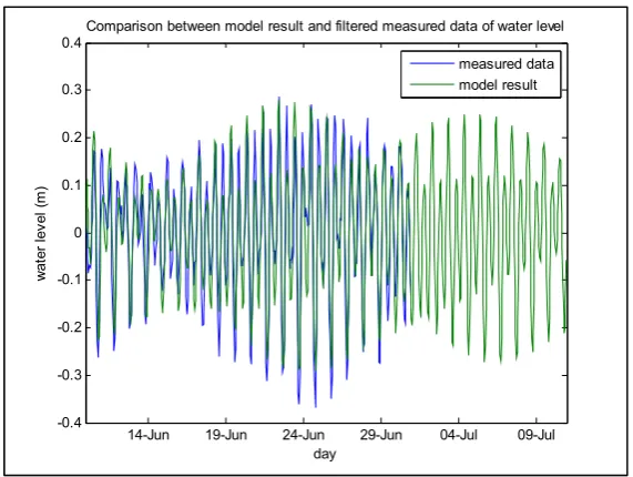
In order to guarantee the reliability, the model should be calibrated against hydrodynamic
274
measurements, such as water level and velocity. To calibrate the model for water level, the available
275
water level data for Songkhla was used (Figure 5). The model results agree with the data in amplitude
276
and phase.
277
278
Figure 5: Comparison between model result and filtered measured data of Songkhla water level
279
during July 1997.
280
Velocity calibration was done using velocity data at two different locations: North and South of Ko
281
Yo Island. The comparison between data and model results for the two points are plotted in Figure 6.
282
The results from North of Koyo show a phase lag of 2 hours comparing to the data, but the amplitude
283
of the tidal currents is well correlated. The South of Koyo results show smaller amplitude when
284
compared to the data, but the difference is very small, less than 0.05 m/s. Despite these small
285
differences, the model was considered well calibrated.
286
287
(a) (b)
288
Figure 6: Comparison between model results and measured data of velocity at a) North of Ko Yo and
289
b) South Ko Yo.
290
291
14-Jun 19-Jun 24-Jun 29-Jun 04-Jul 09-Jul
-0.4 -0.3 -0.2 -0.1 0 0.1 0.2 0.3 0.4
day
w
at
er
le
ve
l (
m
)
Comparison between model result and filtered measured data of water level
measured data model result
29-Jun 00:0029-Jun 12:0030-Jun 00:0030-Jun 12:0001-Jul 00:00 01-Jul 12:00 02-Jul 00:00 -0.4
-0.3 -0.2 -0.1 0 0.1 0.2 0.3 0.4
Time
Ve
lo
ci
ty
(
m
/s
)
Comparison between model result and measured data of velocity North of Ko Yo
model measurement
27-Jun 00:0027-Jun 12:0028-Jun 00:0028-Jun 12:0029-Jun 00:0029-Jun 12:0030-Jun 00:00 -0.3
-0.2 -0.1 0 0.1 0.2 0.3
Time
Ve
lo
ci
ty
(
m
/s)
Comparison between model result and measured data of velocity South of Ko Yo
4. Discussion
292
After calibration, several scenarios were defined to simulate current and future conditions. For
293
each scenario, a period of 15 days was simulated using Delft3D-Flow and Delft3D-WAQ. The
294
scenarios are summarized in Table 1 and Table 2. To represent the river flows, two models were used:
295
GFDL and ECHAM. These models give the current and future conditions, represented by the year
296
2000 and 2100 respectively. The dry month is represented by February, while the wet is October.
297
Because the uncertainty about the river flows, two different percentages of the flow given by the two
298
models were used: 5% and 20%.
299
To represent the sea level rise for the year 2100, the bathymetry for the entire region was
300
deepened by 0.79m, which represents the worst-case estimate of IPCC for the year 2100.
301
302
Table 1 – Simulated scenarios input with 5% of the rivers flows
303
Model GFDL ECHAM
Year 2000 2100 2000 2100 Season wet dry wet dry wet dry wet dry Total Flow 5 0.4 4.6 0.065 6.1 0.15 6.7 0.32 Utaphao 4 0.32 3.68 0.052 4.88 0.12 5.36 0.256 Rattaphum 1 0.08 0.92 0.0057 1.22 0.03 1.34 0.064
304
Table 2 - Simulated scenarios input with 20% of the rivers flows
305
Model GFDL ECHAM
Year 2000 2100 2000 2100 Season wet dry wet dry wet dry wet dry Total Flow 20 2 18.4 0.26 24.4 0.6 26.8 1.3
Utaphao 16 1.28 14.72 0.208 19.52 0.48 21.44 1.04 Rattaphum 4 0.32 3.68 0.052 4.88 0.12 5.36 0.26
The maximum velocities at the inlet are represented in Table 3 and Table 4 According to the
306
results, there are no significant changes of velocities at the inlet between the dry and wet months or
307
between scenarios with 5% and 20% of river flow, which means that probably the river discharges
308
doesn’t have high influence on velocities at the inlet. Comparing the current and future scenarios, it
309
can be observed that the maximum velocities in the future will be higher than today due to sea level
310
rise, this increase corresponds to around 20% for all cases. However, it is likely that the inlet
311
morphology will also change in the future in order to preserve inlet equilibrium velocities of around
312
1 ms-1.
313
Table 3 - Maximum velocities at the inlet for the scenarios with 5% of river flow
314
GFDL ECHAM
2000 2100 2000 2100
Season wet dry wet dry wet dry wet dry Maximum velocity (inlet) 1.05 1.02 1.24 1.25 1.06 1.02 1.24 1.25
Table 4 - Maximum velocities at the inlet for the scenarios with 20% of river flow
315
GFDL ECHAM
2000 2100 2000 2100
4.1 Flushing Time
317
The flushing time results are summarized in Table 5 and Table 6. The results show that for all
318
cases, the flushing time for wet months is smaller than for dry months (22% for 5% of river flow and
319
111% for the 20% of river flow). Scenarios with 20% of river flow also showed smaller flushing times
320
comparing with the 5% ones. The rivers help to flush the lagoon so its flow is inversely proportional
321
to flushing time. Also, the flushing time will decrease in future scenarios of sea level rise; this decrease
322
will be different, depending on the river flow changes. When the river flow increase, which is the
323
case of ECHAM model, the flushing time have a higher decrease.
324
Table 5 - Calculated flushing time for the scenarios with 5% of river flow
325
GFDL ECHAM
2000 2100 2000 2100 Season wet dry wet dry wet dry wet dry Flushing time (h) 270.05 319.15 199.87 267.36 318.92 331.02 200.70 267.38
Table 6 - Calculated flushing time for the scenarios with 20% of river flow
326
GFDL ECHAM
2000 2100 2000 2100 Season wet dry wet dry wet dry wet dry Flushing time (h) 146.6 281.8 110.4 235.9 134.5 281.2 102.7 236.1
327
4.2 Salinity
328
All the simulations showed a similar salinity distribution, with different magnitudes Figure 7
329
shows the result of depth average salinity of the entire lagoon for the scenarios using ECHAM model
330
for the instant 13th October 2000 at 22:00h. This result shows a salinity of 35 psu outside the lagoon.
331
Inside the lagoon the salinity decreases near the rivers, with a minimum of 25 psu close to the river
332
mouth.
333
334
Figure 7: Result for depth average salinity for Scenario ECHAM - 2000 - wet for the instant 13th
335
October 2000 at 22:00h
336
The mean salinity for a point in the center of the lagoon was calculated and the results are
337
summarized in Table 7 and Table 8. For both models, the results showed a difference in salinities
338
between wet and dry months. The wet months presents lower salinity than the dry months for all the
339
more than 15 psu. The salinity during the dry months didn’t show much change for all the scenarios.
341
However, it should be noted that CC driven variation in evaporation was not considered in these
342
simulations.
343
Table 7 - Mean salinity at a point in center of the lagoon for the different scenarios with 5% river flow
344
GFDL ECHAM
2000 2100 2000 2100 Season wet dry wet dry wet dry wet dry Salinity (psu) 31.52 34 31.44 34 33.24 34 31.13 34
Table 8 - Mean salinity at a point in center of the lagoon for the different scenarios with 20% river flow
345
GFDL ECHAM
2000 2100 2000 2100
Season wet dry wet dry wet dry wet dry Salinity (psu) 15.8 33.0 17.14 33.0 13.05 33.0 14.3 32.9
4.3. Stratification
346
The stratification of the lagoon is defined as the difference between the bottom and the top layers
347
of the simulation results. Figure 8 shows this difference for the entire lagoon for the scenarios using
348
river flow derived from the ECHAM model for the instant 13th October 2000 at 22:00h. It can be
349
observed that there is no stratification in the east part of the lagoon. The greatest stratification is found
350
on the western part, especially close to the river mouths, where it can reach 15 psu.
351
352
Figure 8: Difference between the bottom and the top layer of salinity results for Scenario ECHAM -
353
2000 - wet for the instant 13th October 2000 at 22:00h
354
The maximum stratification for a point located in the west part of the lagoon was calculated and
355
the results are summarized in Table 9 and Table 10. This point was chosen because is a point with
356
significant stratification and not very close to the rivers mouths. The results show that the
357
stratification for this point is greater during wet season. Comparing current with future scenarios,
358
during wet months stratification decreases in the future for the simulations with 5% of river flow and
359
it increases in the simulations with 20% of river flow. For the dry months, all simulations showed an
360
increase in stratification in future. It should be noted that CC driven variations in wind were not
361
Table 9 – Average Difference salinity at a point in the western part of the lagoon for the different
363
scenarios with 5% of river flow
364
GFDL ECHAM
2000 2100 2000 2100
Season wet dry wet dry wet dry wet dry
Difference (psu) 1.45 0.33 1.09 0.83 1.72 0.29 1.27 0.81
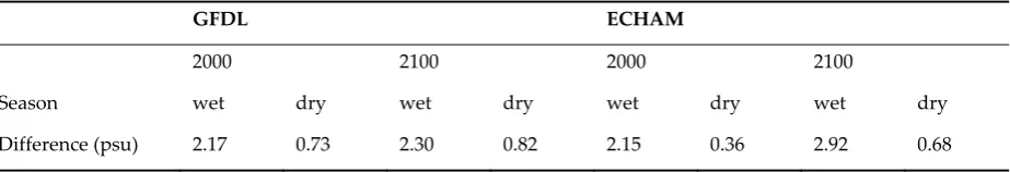
Table 10 - Average Difference salinity at a point in the western part of the lagoon for the different
365
scenarios with 20% of river flow
366
GFDL ECHAM
2000 2100 2000 2100
Season wet dry wet dry wet dry wet dry
Difference (psu) 2.17 0.73 2.30 0.82 2.15 0.36 2.92 0.68
367
5. Conclusions
368
The proposed framework is a useful tool to assess Climate Change impacts. The five steps
369
provide a comprehensive analysis from atmospheric modeling, climatic downscaling to impacts in
370
coastal lagoons. The river flow obtained using dynamically downscaled projections from two global models
371
GFDL and ECHAM showed different results. The year of 2000, both showed the same behavior, but different
372
magnitudes. For the year 2100 they showed opposite behavior, ECHAM predicts an increase of river flow,
373
while GFDL predicts a decrease. The high variability associated to the river flow and uncertainties of long
374
prediction are possible reasons for this difference.
375
Some scenarios were designed to simulate current and future scenarios for the region during dry and wet
376
seasons and for river flow of 5% and 20% of the two available models, with a total of 16 simulations. The
377
results show that circulation in Thale Sap Songkhla is strongly influenced by the lake geometry. The strong
378
flow, coming from the lake entrance, deflects to the north and the south of Ko Yo. The velocities at the entrance
379
channel are around 1m/s and the simulations show an increase of 20% for the year 2100 (in the absence of
380
morphological adjustments, which were not simulated here).
381
Flushing time, salinity intrusion and stratification, are useful indicators to quantify the impacts of CC in
382
coastal lagoons. For the specific case of Songkhla Lagoon, the flushing time is smaller during wet months,
383
because of the higher river flows and is expected to decrease for future scenarios due to the sea level rise.
384
Salinity has different values for wet and dry months, being higher during dry months because the weaker river
385
flows. Stratification results showed a higher stratification during wet season. The results suggest distinct
386
behavior for future scenarios, during wet months the stratification can decrease or increase depending on river
387
flow considerations. During dry months, it will increase for future scenarios. This result was not sufficient and
388
further analysis should be done to find the reasons for this behavior.
389
For future modeling efforts, there is an urgent need for high quality simultaneous measurements of water
390
level, velocity, and salinity at several points spread across the lagoon over a duration of at least 30 days during
391
both the wet and dry seasons. River discharge data and atmospheric data, such as: wind, evaporation, rainfall,
392
solar incidence should also be measured.
393
The main limitation of this study is the lack of data for the region. Due to this limitation, the results of this
394
study should be interpreted in a qualitative way. The comparison between the scenarios are valid, but the
395
absolute values needs further investigation.
396
Acknowledgments: The authors acknowledge the Erasmus Mundus program CoMEM (Coastal, Marine
397
Engineering and Management) and the Lamminga Fund, for the scholarship during the development of this
398
Author Contributions: Bruno Primo led the project, performed all the Delft3D and Delft3D-WAQ modelling,
400
did all the analysis and co-wrote the paper with Fernanda Achete. Sarith Mahanama performed all the
401
downscaled river flow modelling, Marcus Thatcher and Mark Hemer provided the dynamically downscaled
402
GCM output, Sutat Weesakui and Trang Duong collated and provided the field data required for model
403
validation.
404
Conflicts of Interest: The authors declare no conflict of interest.
405
References
406
1. Bruun, P., Gerritsen, F. Stability of Coastal Inlets. North-Holland Publishing Co., Amsterdam, 1960, 123
407
pp.
408
2. Kjerfve, B., Coastal Lagoon Processes. Elsevier Science Publishers, Amsterdam, 1994, 577pp.
409
3. Barnes, H. Coastal lagoons, Cambridge University Press. 1980 106pp.
410
4. FitzGerald, D.M., Fenster, M.S., Argow, B.A., Buynevich, I.V. Coastal impacts due to sea-level rise.
411
Annu. Rev. Earth Planet Sci. 2008, 36, 601–647.
412
5. Anthony, A., J. Atwood, P. August, C. Byron, S. Cobb, C. Foster, C. Fry, A. Gold, K. Hagos, L. Heffner,
413
D. Q. Kellogg, K. Lellis-Dibble, J. J. Opaluch, C. Oviatt, A. Pfeiffer-Herbert, N. Rohr, L. Smith, T.
414
Smythe, J. Swift, and N. Vinhateiro. Coastal lagoons and climate change: ecological and social
415
ramifications in U.S. Atlantic and Gulf coast ecosystems. Ecology and Society, 2009 14(1): 8.
416
6. Kjerfve, B. and Magill, K.E., Geographic and hydrodynamic characteristics of shallow coastal lagoons.
417
Marine Geology, 1989 88, 187-199
418
7. Nichols, M.M., and Allen, G., Sedimentary processes in coastal lagoons. Coastal lagoon research, present
419
and future. 1981, pp. 77-187
420
8. Haines, P. Anticipated Response of Coastal Lagoons to Sea Level Rise. IPWEA National Conference
421
August 2008
422
9. Lesser, G., An Approach to Medium-term Coastal Morphological Modeling, PhD thesis,
UNESCO-423
IHE/Delft University of Technology, 2009 (ISBN 978-0-415-55668-2).
424
10. DeVriend, H.J., Zyserman, J., Nicholson, J., Roelvink, J.A., Pechon, P., Southgate, H.N., Medium term
425
2DH coastal area modelling. Coast. Eng. 1993 21, 193–224.
426
11. Dabees, M., Kamphuis, J.W., ONELINE: efficient modeling of 3-D beach change. Proceedings of the
427
27th International Conference on Coastal Engineering, Sydney, Australia, ASCE, 2000 pp. 2700–2713
428
12. Hanson, H., Aarninkhof, S., Capobianco, M., Jimenez, J.A., Larson, M., Nicholls, R., Plant, N.,
429
Southgate, H.N., Steetzel, H.J., Stive, M.J.F., De Vriend, H.J., 2003. Modelling coastal evolution on early
430
to decadal time scales. J. Coast. Res. 19 (4), 790–811.
431
13. Roelvink, J.A., Coastal morphodynamic evolution techniques. Coast. Eng. 2006, 53, 277–287.
432
14. Ranasinghe, R., Assessing Climate change impacts on Coasts: A Review. Earth Science Reviews, 2016,
433
160, 320-332.
434
15. Duong T., Ranasinghe R., Thatcher M., Mahanama S., Wang Z., Dissanayake P., Hemer M.,
435
Luijendijk A., Bamunawala J., Roelvink D. and Walstra D. 2018. Assessing climate change impacts on
436
the stability of small tidal inlets: Part 2 – data rich environments. Marine Geology, Vol 395, 65-81
437
16. McGregor J, C-CAM: Geometric aspects and dynamical formulation. CSIRO Marine and Atmospheric
438
Research Tech Paper 2005a, 70, 43 pp.
439
17. McGregor J and Dix M. An updated description of the conformal cubic atmospheric model. High
440
resolution Simulation of the Atmosphere and Ocean. K. Hamilton and W. Ohfuchi, Eds. 2008, Springer,
441
51-76.
442
18. Schmidt F., Variable fine mesh in spectral global models. Beitr. Phys. Atmos. 1977, 50, 211-217.
443
19. Rotstayn L., A physically based scheme for the treatment of stratiform clouds and precipitation in large
444
scale models. I: Description and evaluation of the microphysical processes. Quart. J. Roy. Meteor. Soc.,
445
1997, 123, 1227-1282.
446
20. McGregor, J. L. A new convection scheme using a simple closure. In Current issues in the
447
parameterization of convection, BMRC Research Report, 2003, 93, 33–36.
448
21. Kowalczyk E.; Garratt J.; Krummel P. Implementation of a soil-canopy scheme into the CSIRO GCM –
449
Regional aspects of the model response. CSIRO Martine and Atmospheric Research Tech Report, 1994,
450
22. McGregor, J. L.; Gordon H. B.; Watterson, I. G.; Dix, M. R; Rotstayn, L. D., The CSIRO 9-level
452
atmospheric general circulation model. CSIRO Div. Atmospheric Research Tech. 1993, Paper No. 26, 89
453
pp.
454
23. Holtslag A and Boville B, Local versus non-local boundary layer diffusion in a global climate model.
455
J. Climate, 1993, 6, 1825-1842.
456
24. Smith R, A scheme for predicting layer clouds and their water content in a General Circulation Model.
457
Quart. J. Roy. Meteor. Soc. 1990, 116, 435-460.
458
25. Chouinard C, Beland M and McFarlane N, A simple gravity wave drag parameterization for use in
459
medium-range weather forecast models. Atmos-Ocean, 1986, 24, 91-110.
460
26. Lacis A and Hansen J, A parameterisation of the absorption of solar radiation in the Earth’s
461
atmosphere. J. Atmos. Sci, 1974 31, 118-133.
462
27. Schwarzkopf, M.; Fels, S. The simplified exchange method revisited: An accurate, rapid method for
463
computation of infrared cooling rates and fluxes. J. Geophys. Res. 1991, 96, 9075-9096.
464
28. Wang Y, Leung L, McGregor J, Lee D, Wang W, Ding Y and Kimura F, Regional climate modeling:
465
Progress, challenges and prospects. J. Meteor. Soc. Japan. 2004, 82, 1599-1628.
466
29. Koster, R.D., Suarez, M.J., Ducharne, A., Stieglitz, M., Kumar, P., A catchment-based approach to
467
modeling land surface processes in a general circulation model: 1. Model structure. J. Geophys. Res.
468
2000, 105 (20), 24,809–24,822.
469
30. Ducharne, A., R.D. Koster, M.J. Suarez, M. Stieglitz, and P. Kumar. A catchment-based approach to
470
modeling land surface processes in a GCM. Part 2: Parameter estimation and model demonstration.
471
Journal of Geophysical Research Atmospheres, 2000, 105(D20): 24823-24838.
472
31. Mahanama, P.P. Sarith & D. Koster, Randal & H. Reichle, Rolf & Zubair, Lareef. The role of soil
473
moisture initialization in subseasonal and seasonal streamflow prediction – A case study in Sri Lanka.
474
Advances in Water Resources. 2008, 31. 1333-1343. 10.1016
475
32. Lesser, G., Roelvink, J.A., Van Kester, J.A.T.M., Stelling, G.S., Development and validation of a
three-476
dimensional morphological model. Coast. Eng. 2004, 51, 883–915.
477
33. Pornpinatepong, S.; Tanaka, H.; Takasaki, M. Application of 2-D Vertically Averaged Boundary-Fitted
478
Coordinate Model of Tidal Circulation in Thale Sap Songkhla, Thailand. Walailak J Sci & Tech 2006 3(1):
479
105-118
480
34. Viet, N. T., Tanaka, H., Takasaki, M. and Yamaji, H. In-situ investigation and simulation of water
481
quality changes in Songkhla Lake, Thailand. Proceedings of the 4th Asian and Pacific Coasts Vol. 4.,
482
2007 Nanjing, China.
483
35. Aubrey, D. G.; McSherry, T. R., and Eliet, P.P., Effects of multiple inlet morphology on tidal exchange:
484
Waquoit Bay, Massachussettes. In: Aubrey, D. G. and Giese, G. S. (eds.), Formation and Evolution of