Article
1
Development and Evaluation of a
Reynolds-2
Averaged Navier-Stokes Solver in WindNinja for
3
Operational Wildland Fire Applications
4
Natalie S. Wagenbrenner 1,*, Jason M. Forthofer 1, Wesley G. Page 1, and Bret W. Butler 1
5
1 US Forest Service, Rocky Mountain Research Station, Missoula Fire Sciences Laboratory, 5775 W Highway
6
10, Missoula, MT 59808, USA; [email protected] (J.M.F.); [email protected] (W.G.P);
7
[email protected] (B.W.B.)
8
* Correspondence: [email protected]
9
10
Abstract: An open source computational fluid dynamics (CFD) solver has been incorporated into
11
the WindNinja modeling framework widely used by wildland fire managers as well as researchers
12
and practitioners in other fields, such as wind energy, wind erosion, and search and rescue. Here
13
we describe incorporation of the CFD solver and evaluate its performance compared to the
14
conservation of mass (COM) solver in WindNinja and previously published large-eddy simulations
15
(LES) for three field campaigns conducted over isolated terrain obstacles of varying terrain
16
complexity: Askervein Hill, Bolund Hill, and Big Southern Butte. We also compare the effects of two
17
important model settings in the CFD solver and provide guidance on model sensitivity to these
18
settings. Additionally, we investigate the computational mesh and difficulties regarding terrain
19
representation. Two important findings from this work are: (1) the choice of discretization scheme
20
for advection has a significantly larger effect on the simulated winds than the choice of turbulence
21
model and (2) CFD solver predictions are significantly better than the COM solver predictions at
22
windward and lee side observation locations, but no difference was found in predicted speed-up at
23
ridgetop locations between the two solvers.
24
Keywords: microscale wind modeling; RANS modeling; complex terrain; wildland fire
25
26
1. Introduction
27
WindNinja is a microscale diagnostic wind model developed for and widely used in operational
28
wildland fire applications both in the United States (U.S.) and abroad [1-2]. Microscale wind
29
modeling is used for a variety of tasks in wildland fire management including planning,
30
reconstructing past events, and exploring what-if scenarios. Often many, even thousands of
31
simulations, must be run in a short time frame depending on the modeling objectives. WindNinja
32
was developed over 15 years ago specifically for these types of tasks and, to our knowledge, is the
33
most widely used microscale wind model in wildland fire. WindNinja is embedded within a number
34
of operational systems routinely used by U.S. Interagency Wildland Fire response teams, including
35
the Wildland Fire Decision Support System [3] and FlamMap [4] and is also regularly used as a
stand-36
alone model by both fire managers and on-the-ground firefighters.
37
The original version of WindNinja employs a numerical solver that enforces conservation of
38
mass (hereafter referred to as the ‘COM’ solver) to simulate mechanical effects of the terrain on the
39
near-surface wind [1]. Evaluations against field data have shown that the COM solver can simulate
40
many terrain-induced near-surface flow effects, including speed-up over ridges, terrain channeling,
41
and reduced lee side velocities [1-2, 5]; however, it is well-documented that COM solvers, including
42
the one in WindNinja, have difficulties simulating the flow field in regions where momentum effects
43
dominate, notably on the lee side of terrain obstacles where flow separation can lead to areas of
44
recirculation [1, 6].
45
Due to its success in the operational wildland fire community, WindNinja has been under
46
continuous development and has evolved over the last ten years into a robust wind modeling
47
framework. This framework includes a modern graphical user interface, flexible initialization options,
48
the ability to download data required for model initialization, user-selectable thermal
49
parameterizations, and multiple easy-to-use output products. As a part of ongoing development
50
efforts, a second numerical solver based on computational fluid dynamics (CFD) has been added to
51
the framework. This new solver is similar to the CFD model described by Forthofer et al. [1], but is
52
based on free, open-source software embedded directly within the WindNinja framework. This new
53
CFD solver is expected to improve predictions, particularly in lee side flow regions, with only a
54
marginal increase in computational effort such that simulations are still affordable on typical laptop
55
computers.
56
This paper describes the new CFD solver and provides an initial evaluation of its performance
57
against field measurements, the COM solver in WindNinja, and previously published large-eddy
58
simulation (LES) results. We investigate two commonly-used discretization schemes for the
59
advection term in the momentum equation, three turbulence model configurations, and assess the
60
impact of these numerical settings on the results. The effect of the numerical mesh on results is also
61
discussed. The specific goals of this study are to: (1) determine the most appropriate combination of
62
numerical settings for the CFD solver and (2) compare the CFD solver predictions to predictions from
63
the COM solver and LES observations in order to put the CFD results into context and demonstrate
64
the error associated with each solver type.
65
2. WindNinja Framework
66
The WindNinja code is written primarily in the C/C++ programming language and is open
67
source and available on GitHub (github.com/firelab/windninja). It is cross-platform and runs on both
68
the Linux and Windows operating systems. The framework includes a graphical user interface (GUI),
69
command line interface (CLI), and an application programming interface (API) that allows efficient
70
integration into other software. Additional model information can be found at
71
weather.firelab.org/windninja.
72
WindNinja has seen broad and increasing use (e.g., more than 7 million simulations in 30
73
countries during 2018), largely due to its user-friendly interface and suite of auxiliary features that
74
minimize the effort required by the user and enhance the user experience. WindNinja has simple
75
input requirements, which include a digital elevation model for the terrain, specification of the
76
dominant vegetation in the domain, and an input wind. All of these inputs can be downloaded from
77
online sources via WindNinja. WindNinja allows three options for specification of the initial wind:
78
(1) a domain-average wind, which is an average wind for the domain specified at a single height
79
above the ground; (2) wind information from one or more observation points (e.g., weather stations);
80
and (3) a coarser resolution wind field from a numerical weather prediction model.
81
The core of the WindNinja framework are the two numerical solvers used to solve for the
82
flow field. Both solve for a neutrally-stratified flow; however, thermal parameterizations are available
83
to approximate some thermal effects including diurnal slope winds and non-neutral atmospheric
84
stability. The slope flow parameterization is described in Forthofer et al. [7]. The stability
85
parameterization adjusts the Gauss precision moduli in the governing equation solved in the COM
86
solver based on the estimated Pasquill stability class following recommendations in Chan and
87
Sugiyama [8] and Homicz [9]. As described in Forthofer et al. [1], the Gauss precision moduli control
88
the relative amount of change allowed by the solver in the horizontal and vertical directions. If the
89
stability parameterization is not used, the Gauss precision moduli are set to 1, which creates a
90
numerical situation representative of neutral atmospheric conditions.
91
Since the current implementation of the stability parameterization is based on modifications to
92
parameters in the governing equation solved in the COM solver, this parameterization is not
93
available for use with the CFD solver. Future work is intended to allow non-neutral simulations with
the CFD solver. The diurnal slope flow parameterization is incorporated into CFD simulations by
95
first running a neutral CFD simulation, then adding in the diurnal slope flow component to the CFD
96
solution in each cell of the domain, and finally running a COM simulation on the slope flow-adjusted
97
CFD solution. This chaining together of CFD and COM simulations allows approximation of
98
thermally-driven slope flows without explicitly solving an energy equation in the CFD solver, which
99
keeps the simulation times affordable.
100
3. CFD Solver Description
101
The CFD solver in WindNinja is based on OpenFOAM version 2.2.0 [10] (www.openfoam.org).
102
The formulation of this solver is similar to that of the mass and momentum conserving solver
103
described in Forthofer et al. [1] which has been previously used in operational wildland fire
104
applications under the name “WindWizard”. Differences between the Fluent-based Forthofer et al.
105
[1] solver and the CFD solver described here include the computational mesh structure, turbulence
106
closure scheme, treatment of the ground boundary condition, and that all code used in the current
107
CFD model is free and open source, which allows WindNinja to continue to be released without
108
licensing restrictions or fees. This last point regarding software licensing is a major issue for
109
operational wildland fire, particularly for government personnel who may not have access to funds
110
or approval to purchase software licenses for their work.
111
As in Forthofer et al. [1], the flow is assumed to be steady, viscous, incompressible, turbulent,
112
and neutrally-stratified, and the Coriolis force is ignored. WindNinja employs the simpleFoam solver,
113
which is an implementation of the semi-implicit method for pressure-linked equations (SIMPLE)
114
method, to approximate solutions to the steady-state, incompressible Reynolds-Averaged
Navier-115
Stokes (RANS) equations. Using the Boussinesq approximation [11], the RANS equations are:
116
117
𝜕𝑢̅𝑖 𝜕𝑥𝑖 = 0118
119
𝜕(𝑢̅𝑗𝑢̅𝑖) 𝜕𝑥𝑗= −1 𝜌 𝜕𝑝̅ 𝜕𝑥𝑖 + 𝜕 𝜕𝑥𝑗 (𝜐 [𝜕𝑢̅𝑖 𝜕𝑥𝑗 + 𝜕𝑢̅𝑗 𝜕𝑥𝑖 ] ) + 𝜕 𝜕𝑥𝑗 (−𝜌𝑢̅̅̅̅̅̅)𝑖′𝑢𝑗′
120
121
In Eqs. (1) and (2) 𝑢̅𝑖 and 𝑢̅𝑗are the time-averaged velocity components in the i and j coordinate
122
directions, 𝑢𝑖′ and 𝑢𝑗′ are the instantaneous velocity components in the i and j coordinate directions,
123
p is pressure, ρ is density, and ν is the laminar viscosity. A two-equation eddy viscosity turbulence
124
model is used to model the contribution of the instantaneous velocity components. This introduces a
125
turbulent viscosity, νt, to account for the effects of the instantaneous velocity components:
126
127
𝜕(𝑢̅𝑗𝑢̅𝑖)
𝜕𝑥𝑗
= −1 𝜌 𝜕𝑝̅ 𝜕𝑥𝑖 + 𝜕 𝜕𝑥𝑗 (𝜐 + 𝜐𝑡[ 𝜕𝑢̅𝑖 𝜕𝑥𝑗 + 𝜕𝑢̅𝑗 𝜕𝑥𝑖 ])
128
129
Three two-equation turbulence models are investigated, the standard k-epsilon model [12], a
130
modified k-epsilon model that allows production and dissipation of turbulent kinetic energy (TKE)
131
to be out of equilibrium at the ground, and the renormalization group (RNG) k-epsilon model [13].
132
In all cases, the turbulent viscosity is calculated as:
133
134
𝜐𝑡= 𝐶𝜇 𝑘2 𝜀135
136
In Eq. (4) Cµ is a constant (see Table 1), k is the TKE, and ε is the dissipation of TKE. Two
137
additional transport equations are solved, one for k and one for ε. For the standard k-epsilon model
138
the additional equations are:
𝜕(𝑘𝑢̅𝑖) 𝜕𝑥𝑖 = 𝜕 𝜕𝑥𝑗 [𝜐𝑡 𝜎𝑘 𝜕𝑘 𝜕𝑥𝑗 ] + 𝑃 − 𝜀
141
142
𝜕(𝜀𝑢̅𝑖) 𝜕𝑥𝑖 = 𝜕 𝜕𝑥𝑗 [𝜐𝑡 𝜎𝜀 𝜕𝜀 𝜕𝑥𝑗] + 𝐶𝜀1
𝑃𝜀 𝑘 − 𝐶𝜀2
𝜀2
𝑘
143
144
In Eq. (5) P is the production of TKE and is given by:
145
146
𝑃 = 2𝜐𝑡𝑆𝑖𝑗𝑆𝑖𝑗
147
148
where Sij is the mean rate of strain tensor:
149
150
𝑆𝑖𝑗 = 1 2( 𝜕𝑢̅𝑖 𝜕𝑥𝑗 +𝜕𝑢̅𝑗 𝜕𝑥𝑖 )151
152
The conservation equations are the same for the other two turbulence models, except the
153
modified k-epsilon model uses a wall function for the production term in the dissipation equation
154
and the RNG k-epsilon model treats the constant Cε1 as a variable that depends on the ratio of the
155
production of TKE to its dissipation:
156
157
𝐶𝜀1𝑅𝑁𝐺= 1.42 −
𝜂(1 − (𝜂/4.38)) 1 + 𝛽𝑅𝑁𝐺𝜂3
158
159
where:160
161
𝜂 = √𝑃𝑘/𝜌𝐶𝜇𝑅𝑁𝐺𝜀162
163
and the production of TKE is:
164
165
𝑃𝑘 = 𝜏𝑖𝑗 𝜕𝑢̅𝑖 𝜕𝑥𝑗 = 𝜇𝑡( 𝜕𝑢̅𝑖 𝜕𝑥𝑗 +𝜕𝑢̅𝑗 𝜕𝑥𝑖 )𝜕𝑢̅𝑖 𝜕𝑥𝑗166
167
Model constants are listed in Table 1. The custom OpenFOAM code used in the modified
k-168
epsilon model is available in the WindNinja GitHub repository.
169
170
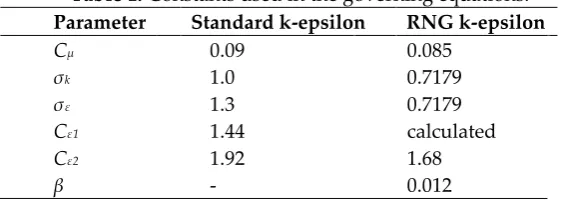
Table 1. Constants used in the governing equations.
171
Parameter Standard k-epsilon RNG k-epsilon
Cµ 0.09 0.085
σk 1.0 0.7179
σε 1.3 0.7179
Cε1 1.44 calculated
Cε2 1.92 1.68
β - 0.012
172
The governing equations are discretized using the finite volume method. Two second-order
173
discretization schemes for advection of the mean wind, linear upwind and the Quadratic Upstream
174
Interpolation for Convective Kinematics (QUICK), are investigated in this work and described in
175
Section 3.1. A first-order bounded Gauss upwind scheme is used for all other advection terms. A
176
second-order Gauss linear limited discretization scheme is used for all diffusion terms.
177
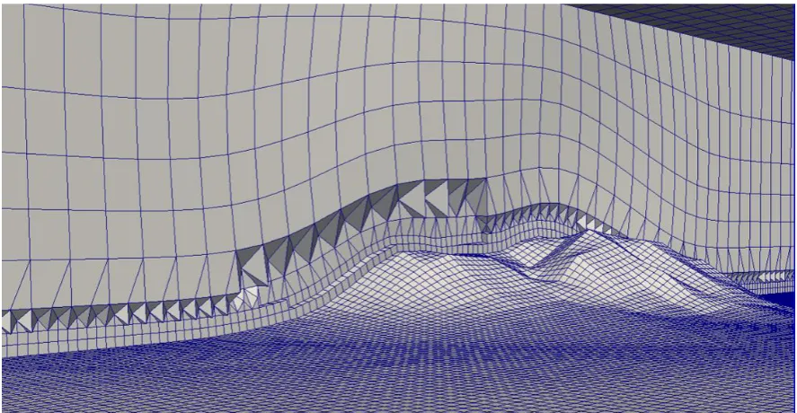
The discretized equations are solved on a terrain-following, unstructured mesh with
178
predominantly hexahedral cells (Figure 1). WindNinja employs a three-step meshing scheme using
179
OpenFOAM mesh generation and manipulation utilities. The number of cells in the mesh is set based
on a user-specified choice of the mesh resolution. The four choices available to the user are ‘coarse’,
181
‘medium’, ‘fine’ or the user can directly set the number of cells to use. The coarse, medium, and fine
182
options correspond to 25K, 50K, and 100K cells, respectively. In the first step of the meshing scheme
183
a blockMesh is generated above the terrain using the blockMesh utility. Then moveDynamicMesh is
184
used to stretch the lower portion of the blockMesh down to the terrain. Finally, the near-ground cells
185
are refined in all three directions using the refineMesh utility. The total number of cells are divided
186
equally between the blockMesh and the refined layer at the ground. The refineMesh utility is
187
executed repeatedly until the specified number of cells have been allocated. This has proven to be a
188
robust approach for automated meshing over complex terrain; however, there are limitations to this
189
approach which are discussed in Section 5.6. A comprehensive investigation of computational mesh
190
quality is beyond the scope of this work, but key considerations regarding the current meshing
191
algorithm are described for the reader and will be the focus of future work.
192
193
194
Figure 1. Slice through the computational mesh used for Big Southern Butte.
195
196
The inlet boundary conditions are specified as follows per Richards and Norris [14]:
197
198
𝑈 = 𝑢∗
𝜅𝑘−𝜀
𝑙𝑛 (𝑧 𝑧0
)
199
200
𝑘 = 𝑢∗
2
√𝐶𝜇
201
202
𝜀 = 𝑢∗
3
𝜅𝑘−𝜀𝑧
203
204
The friction velocity, u*, is calculated as:
205
206
𝑢∗=
𝜅𝑈ℎ
𝑙𝑛 (𝑧ℎ
𝑜)
207
208
where Uh is the input wind velocity at a specified height h above the ground and the von
209
Karman constant, 𝜅, is taken as 0.41.
210
The inlet is terrain-following. The non-inlet side boundaries are set to pressureInletOutlet for
211
velocity and zero-gradient for TKE and dissipation of TKE. The pressureInletOutlet boundary
212
(12)
(13)
(14)
condition assigns a zero-gradient condition if the flow is out of the domain and a velocity based on
213
the flux in the cell face-normal direction if the flow is into the domain. The top boundary is
214
specified as zero-gradient for velocity, TKE, and dissipation of TKE. Rough wall functions are used
215
for the ground boundary condition. The boundary condition imposed at the ground for turbulent
216
viscosity is nutkAtmRoughWallFunction, for TKE is kqRWallFunction, for dissipation of TKE is
217
epsilonWallFunction, and for velocity is a fixed value of 0. The roughness is set based on the
218
vegetation selection in WindNinja, where the choices “grass”, “brush”, and “trees” corresponds to a
219
roughness of 0.01, 0.43, and 1.0 m, respectively.
220
Two departures from the Richards and Norris [14] boundary condition recommendations
221
are that we do not specify a shear stress at the top boundary and we use a value of 0.41 for the von
222
Karman constant, rather than the values determined by the turbulence model, which turn out to be
223
0.433 for the standard k-epsilon model and 0.4 for the RNG k-epsilon model. Implementation of
224
these recommendations will be undertaken in future work.
225
The implemented boundary conditions were tested on a flat terrain case and the inlet and
226
outlet profiles are compared (Figure 2). The results shown in Fig. 2 are for the standard k-epsilon
227
turbulence model with the linear upwind discretization scheme. The horizontal extent of the
228
computational mesh is 800 x 400 m, with a top height of 80 m above sea level, and cell horizontal
229
spacing and cell height of 1 m in the near-ground cells. For a horizontally homogenous flat terrain,
230
the inlet and outlet profiles should be identical. There is a slight decay in the velocity profile over
231
the length of the domain (Figure 2), which could potentially be mitigated with specification of a
232
shear stress rather than zero-gradient at the top boundary as suggested by Richards and Norris [14].
233
The kink in the near-ground layer of the TKE profile is commonly observed in RANS modeling and
234
may be due to one or more issues, including the near-ground cell height, inconsistency in the
235
discretization used for TKE production term versus that used for the shear stresses in the
236
momentum equation, or perhaps the turbulence model itself [14-16]. Future work will investigate
237
improvements to the top boundary condition and approaches to mitigate the kink in the TKE
238
profile, but overall, these results are satisfactory for our typical use case in wildland fire
239
applications.
240
241
242
Figure 2. Profiles for (a) velocity, (b) turbulent kinetic energy (TKE), and (c) dissipation of TKE
243
over flat terrain.
244
245
4. Methods
246
4.1. CFD Configuration and Settings Investigated
247
Preliminary testing was conducted with meshes containing up to 2M cells, but no appreciable
248
differences were found as compared with results from meshes built using the fine mesh setting in
249
WindNinja. Therefore, all CFD simulations were run with a fine mesh resolution, corresponding to
100K cells. Mesh considerations and terrain representation are further discussed in Section 5.6. The
251
diurnal slope flow parameterization was not used. The vegetation option was set to “grass”, which
252
corresponds to a roughness length of 0.01 m. The “domain average” initialization method was used to
253
initialize the CFD simulations using an average wind speed and direction measured at a single height
254
above ground level at an upstream location at each site.
255
Two second-order discretization schemes are investigated for the advection of the mean wind, the
256
linear upwind scheme and the QUICK scheme. The linear upwind scheme, which is the simplest and
257
most commonly used second-order scheme, uses linear interpolation from the nearest upwind cell
258
center [17]. The QUICK scheme uses a parabola to approximate the profile using the two nearest
259
upwind cell centers. Three k-epsilon-based turbulence models are investigated, the standard k-epsilon
260
model, a modified k-epsilon model that allows production and dissipation of TKE to be out of
261
equilibrium at the ground, and the RNG k-epsilon model as described in Section 3. Table 2 summarizes
262
the settings investigated and provides abbreviations for the six combinations used throughout the
263
paper.
264
265
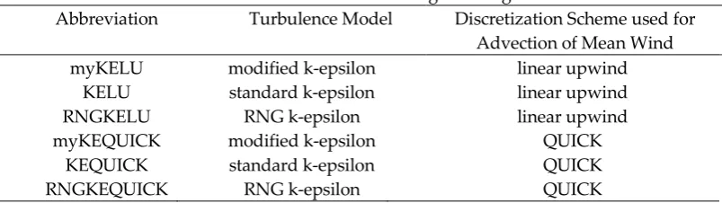
Table 2. CFD settings investigated.
266
Abbreviation Turbulence Model Discretization Scheme used for Advection of Mean Wind myKELU modified k-epsilon linear upwind
KELU standard k-epsilon linear upwind
RNGKELU RNG k-epsilon linear upwind
myKEQUICK modified k-epsilon QUICK
KEQUICK standard k-epsilon QUICK
RNGKEQUICK RNG k-epsilon QUICK
267
4.2. COM Settings
268
WindNinja version 3.5.3 was used for the COM simulations. The diurnal slope flow
269
parameterization was not used. The non-neutral stability parameterization was used only for the
270
Askervein Hill case, which had slightly stable atmospheric conditions (see Section 4.3.1). As with the
271
CFD solver, the fine mesh resolution option was used (which corresponds to 20K cells in the COM
272
mesh), the vegetation option was set to “grass”, and the “domain average” initialization method was
273
used.
274
4.3. Field Observations
275
We evaluate the CFD and COM solvers against data from three field campaigns. Two are classic
276
benchmark datasets, Askervein Hill [18-19] and Bolund Hill [20-21]. The third site, Big Southern Butte
277
[22], represents a more complex geometry with steeper slopes, higher ridgetops, and terrain
278
bifurcations that are more representative of rugged terrain where wildland fires frequently occur, but
279
is surrounded by relatively simple, flat terrain which eases characterization of the approach flow and
280
minimizes issues regarding model boundary conditions. Results are also compared with published
281
LES results for Askervein Hill and Bolund Hill. We are not aware of published LES results for Big
282
Southern Butte.
283
4.3.1. Askervein Hill
284
Askervein Hill (57°11.313’N, 7°22.360’W) is a geometrically-simple hill rising 108 m above the
285
surrounding terrain with a horizontal scale of about 3000 m (Figure 3a). Data were collected at 10 m
286
above ground level along three transects, Lina A, Line AA, and Line B (Figure 3a). The MF03-D and
287
TU03B datasets [19] are used for evaluations. The average approach flow measured at a reference
288
location 3 km upstream was 8.9 m s-1 from a direction of 210°. The atmospheric stability was slightly
289
stable (Figure 3b) with average Richardson numbers between -0.0110 and -0.0074. The ground
roughness length was estimated as 0.03 m [23]. Elevation data at 23-m horizontal resolution on a 6 x
291
6 km domain from Walmsley and Taylor [24] are used for the simulations.
292
293
294
Figure 3. Askervein Hill (a) terrain and measurement locations with axes labeled in meters
295
with north toward the top of the figure and (b) the observed velocity profile measured at an
296
upwind reference station compared to logarithmic and power law profiles; reproduced with
297
permission from Forthofer et al. [1].
298
299
Characteristics of the computational mesh are shown in Table 3. The horizontal extent of the
300
CFD computational mesh is 6 x 6 km with the hill roughly centered in the domain. The mesh top
301
height is 727 m above sea level (Table 3). The average horizontal spacing and cell height of the
near-302
ground cells is 20 m. The COM mesh has the same horizontal extent as the CFD mesh, but has a 742
303
m top height, 43 m horizontal spacing, and a cell height of 0.4 m in the near-ground cells. The
non-304
neutral stability parameterization was used for the COM simulation to approximate a slightly stable
305
atmosphere as measured at the upstream reference site.
306
307
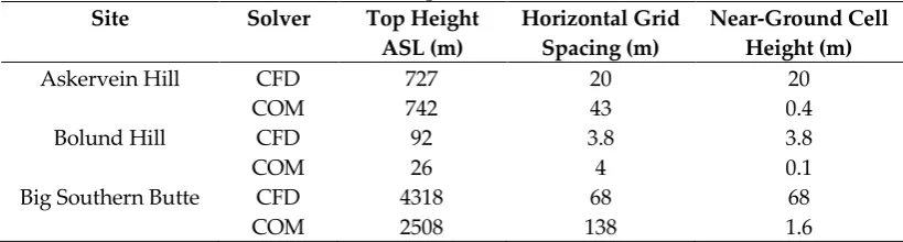
Table 3. Computational mesh characteristics.
308
Site Solver Top Height
ASL (m)
Horizontal Grid Spacing (m)
Near-Ground Cell Height (m)
Askervein Hill CFD 727 20 20
COM 742 43 0.4
Bolund Hill CFD 92 3.8 3.8
COM 26 4 0.1
Big Southern Butte CFD 4318 68 68
COM 2508 138 1.6
309
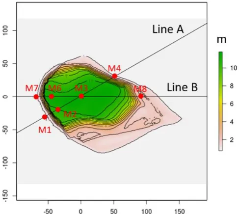
4.3.2. Bolund Hill
Bolund Hill (55°42.21’N, 12°5.892’E) is smaller than Askervein Hill, with only 12 m of relief and
311
a horizontal scale of about 200 m, but it has a steep, cliff-like west face, which makes its geometry
312
slightly more complex (Figure 4). Measurements were made along two transects, Line A and Line B
313
(Figure 4). Three cases from the blind comparison study described in Bechmann et al. [21] are chosen
314
for this work (Table 4). The chosen cases are cases 1, 3, and 4, which correspond to wind speeds and
315
directions of 10.9 m s-1 from 270°, 8.7 m s-1 from 239°, and 7.6 m s-1 from 90°, respectively. The
316
upstream roughness was estimated as 0.0003 m for cases 1 and 3 (approach flow over water) and
317
0.015 m for case 4 (approach flow over land) [21]. Atmospheric stability was characterized as
near-318
neutral for all three cases [21]. Elevation data with a horizontal resolution of 0.25 m and a horizontal
319
extent of 800 x 400 m are used for the simulations.
320
321
322
Figure 4. Bolund Hill terrain and measurement locations. Axes labels are in meters and north
323
is toward the top of the figure.
324
325
Table 4. Bolund Hill cases investigated.
326
Case Wind Speed (m s-1) Wind Direction (°)
1 10.9 270
3 8.7 239
4 7.6 90
327
The CFD mesh has a horizontal extent of 800 x 400 m with the hill centered in the domain. The
328
mesh top height is 92 m above sea level (Table 3). The average horizontal spacing and cell height of
329
the near-ground cells is 3.8 m (Table 3). The COM mesh has the same horizontal extent as the CFD
330
mesh, but has a top height of 26 m, 4 m horizontal grid spacing, and a near-ground cell height of 0.1
331
m (Table 3).
332
4.3.3. Big Southern Butte
333
Big Southern Butte (43°24.083’N, 113°01.433’W) is a tall, isolated mountain and substantially
334
more geometrically complex than Askervein Hill or Bolund Hill (Figure 5). It has a vertical relief of
335
800 m and a horizontal scale of about 4 km. The butte is characterized by a mix of slope angles and
336
multiple bifurcations with ridges and valleys of various sizes forming the sides of the butte. As with
337
Askervein and Bolund hills, the butte is covered predominantly by grass, although there are scattered
338
trees in some locations at the higher elevations. The butte is surrounded by flat terrain covered by
339
grass and small shrubs for more than 50 km in all directions.
342
Figure 5. Big Southern Butte terrain and measurement locations. Panel (a) is zoomed in on the
343
butte and (b) shows the full study area and the location of reference sensor R2. Axes labels are in
344
meters and north is toward the top of the figure.
345
346
The data used for evaluation were collected during the field campaign described in Butler et al.
347
[22]. Wind speed and direction were measured at 3 m above ground level at 53 locations on and
348
around the butte (Figure 5). Here we use the 10-min averaged winds at 1700 LT on 18 July 2010 as
349
the evaluation case. This is the same case investigated as the externally forced flow event in
350
Wagenbrenner et al. [5]. During this period the approach flow was relatively steady (Figure 6b-c) and
351
wind speeds were moderately strong (Figure 6a-b), creating near-neutral atmospheric stability
352
conditions at the surface. The average wind measured at the upstream reference station, R2 (Figure
353
5b), was 8.3 m s-1 from 222° (Figure 6b-c). Elevation data from the Shuttle Radar Topography Mission
354
(SRTM) dataset [25] covering an extent of 19 x 20 km at 30 m horizontal resolution are used for the
355
simulations.
358
Figure 6. Instantaneous wind speeds measured at Big Southern Butte on 18 July 2010 at (a) all
359
sensors and (b) sensor R2; (c) instantaneous wind direction measured at sensor R2 on 18 July 2010.
360
The blue line indicates 10-min averaged wind speed at the top of each hour. The red line indicates
361
1700 LT.
362
363
The CFD mesh has a horizontal extent of 19 x 20 km with the butte centered in the domain. The
364
mesh top height is 4318 m above sea level (Table 3). The average horizontal grid spacing and cell
365
height of the near-ground cells is 68 m (Table 3). The COM mesh has the same horizontal extent as
366
the CFD mesh, but has a top height of 2508 m, 138 m horizontal grid spacing, and a near-ground cell
367
height of 1.6 m (Table 3).
368
4.4. Evaluation Methods
369
One goal of this study is to determine the most appropriate combination of numerical settings
370
for the CFD solver. Results from the six combinations of numerical settings used in the CFD solver
371
are explored by inspecting raster outputs of the predicted surface wind speeds under each
372
combination of numerical settings at each site. Observed and predicted winds along transects at each
373
site are also inspected. Model performance for the CFD and COM solvers is quantified in terms of
374
the root mean square error (RMSE), mean bias error (MBE) and mean absolute percent error (MAPE):
375
376
𝑅𝑀𝑆𝐸 = [1
𝑁∑(𝜑𝑖
′)2 𝑁
𝑖=1
]
1/2
378
𝑀𝐵𝐸 = 1
𝑁∑ 𝜑𝑖
′ 𝑁
𝑖=1
379
380
𝑀𝐴𝑃𝐸 =1
𝑁∑
|𝜑𝑖′|
𝜑𝑖 𝑁
𝑖=1
× 100
381
382
where ϕ is the observed value, ϕ’ is the difference between predicted and observed, and N is the
383
number of observations. Results from LES conducted by others are included in transect plots for
384
Askervein Hill and Bolund Hill for visual comparisons. The LES predictions are shown for reference
385
but are not included in the statistical analyses.
386
Analyses at Askervein and Bolund hills focus on comparisons of observed and predicted wind
387
speed rather than wind direction. This is primarily because, with the exception of Case 4 at Bolund Hill,
388
the observed data do not include major recirculation regions or other terrain-induced directional
389
changes in the wind to warrant that analysis. The observed flow field at Big Southern Butte is much
390
more complex with multiple recirculation regions and flow channeling around the butte as well as
391
within side drainages on the butte [5,22]. Therefore, analysis at Big Southern Butte includes
392
comparisons of wind speeds and directions, along selected transects roughly parallel to the prevailing
393
wind direction as well as with the full set of observations collected on and around the butte. Although
394
wind direction data are presented for Big Southern Butte, mostly to provide additional context
395
regarding the flow dynamics over the butte, the focus of this work is on wind speed predictions. Future
396
work will specifically explore simulated lee side flow dynamics and representation of flow separation
397
and recirculation.
398
An Analysis of Variance (ANOVA) is used to determine the relative effect of the CFD settings
399
on wind speed error. Specifically, the variability in the dependent variable (predicted – observed) is
400
compared to the effects of three independent variables: the discretization scheme (two levels),
401
turbulence model (three levels), location (three levels), and all two-way interactions at the three field
402
sites. The three location levels correspond to either the windward, ridgetop, or leeward locations of the
403
observations. Square-root and cube-root transformations are applied where necessary to meet the
404
assumptions of normality and homoscedasticity of the residuals. The family-wise error rate for multiple
405
comparisons between the means of the various factors levels is controlled using Tukey’s Honest
406
Significant Difference method [26]. The effect size of each individual independent variable is compared
407
by using the Eta-squared (η2) statistic as computed by the sjstats package in R [27], which is a measure
408
of the proportion of the total variation in the dependent variable that can be attributed to a specific
409
independent variable.
410
The data are also pooled across all three field sites to assess the relative effects of the
411
discretization scheme, turbulence model, location, and solver type (i.e., COM vs. CFD) on predicted
412
error. In this case a linear mixed-effects model is constructed using the lmer function in the lme4
413
package in R [28]. The fixed effects are the discretization scheme, turbulence model, location, and solver
414
type while the random effect was the field site. The relative importance of the independent fixed-effect
415
variables are assessed using the relaimpo package in R [29], which estimates the proportion of the
416
variance explained by the model due to the independent variables.
417
5. Results and Discussion
418
5.1. Askervein Hill
419
5.1.1. CFD-predicted flow patterns in the horizontal plane
420
The CFD-predicted 10-m wind speeds using each of the six combinations of numerical settings are
421
shown in Figure 7. Several notable flow features are evident. All combinations predict a reduction in
422
speed as the flow approaches the hill, speed-up on the ridgetop, and reduced speeds on the lee side of
423
(17)
the hill. The size, magnitude, and shape of each of these regions in the predicted flow field vary with
424
the choice of numerical settings. Noticeably, the choice of discretization scheme appears to have a bigger
425
impact on the flow than the choice of turbulence model, both in terms of the magnitude of the predicted
426
speeds and in the spatial patterns in the flow field, particularly on the lee side of the hill (Figure 7a-c
427
versus d-f).
428
The linear upwind scheme produces less ridgetop speed-up and more speed reduction in the lee
429
of the hill as compared with the QUICK scheme (Figure 7a-c versus d-f). The region of reduced speeds
430
in the immediate lee of the hill is also a broader, more coherent pattern in the flow field in the linear
431
upwind simulations as compared with the same region in the QUICK simulations.
432
Low-velocity streamwise streaks are visible in the flow field on the lee side of the hill for all
433
combinations of numerical settings. The linear upwind scheme produces a broad region of low-velocity
434
flow behind the hill, with a streak extending far downwind of this region (Figs. 7a-c). The QUICK
435
scheme produces multiple narrower streaks in the immediate lee of the hill as compared with the linear
436
upwind scheme (Figure 7d-f). The streaks are most well-defined (sharpest gradient normal to the streak)
437
in the myKE simulations (Figure 7a and d). The KE and RNGKE turbulence models appear to smear
438
out the streaks as compared with the myKE model (Figure 7b-c and e-f versus a and d).
439
440
441
Figure 7. CFD-predicted wind speeds in m s-1 at 10 m AGL over Askervein Hill using (a)
442
myKELU; (b) KELU; (c) RNGKELU; (d) myKEQUICK; (e) KEQUICK; (f) RNGKEQUICK. White
443
crosses indicate measurement locations. Black arrows denote the prevailing wind direction. Axes
444
labels are in meters.
445
446
There is experimental and observational evidence from both turbulence and geomorphological
447
research to suggest that the predicted streamwise low-velocity streaks are real terrain-induced features
448
in the flow field [30-34]. Using RANS modeling, Hesp and Smyth [34] show that, for high Reynolds
449
number flows, dune-shaped terrain features induce paired counter-rotating vortices within the wake
450
region of the mean flow. The paired counter-rotating vortices are the mean flow manifestation of
451
transient von Karman vortex shedding (i.e., alternating detachment of vortices on the lee side of a blunt
452
isolated object). Hesp and Smyth [34] further show that the shape and aspect ratio of the terrain feature
453
affects the structure of the horizontal and vertical flow within the wake region. The hills investigated in
454
this work can be broadly categorized as dune-shaped, and indeed, our simulations also contain paired
counter-rotating vortices in the wake zone. The lee side streamwise streaks visible in our simulations
456
are the convergence zones of these paired vortices.
457
We conclude that the streamwise streaks visible in our simulations are the result of simulated
458
converging counter-rotating vortices within the wake regions; however, it is not clear how strong and
459
well-defined the streaks should be. Development of the most well-defined streaks with the strongest
460
cross-flow gradients (Figure 7a and d) could indicate insufficient turbulent diffusion in the model. If
461
that is the case, then modeling choices which smear out the streaks to some degree would be desirable.
462
Other CFD modeling studies have also reported streaks with varying patterns and strengths associated
463
with topographical features in RANS and time-averaged LES simulations [e.g., 35], but there appears
464
to be little guidance in terms of the realistic representation of these streamwise flow features.
465
5.1.2. Comparisons with observations
466
Inspection of the speed-up profiles along the transects further indicates that the choice of
467
discretization scheme has a bigger effect on the predictions than the choice of turbulence model does,
468
particularly on the lee side of the hill (Figure 8). This is indicated by the tight clustering of lines depicting
469
simulations using the linear upwind scheme (red, orange, and pink lines) versus the QUICK scheme
470
(blue, green, and light blue lines) (Figure 8). The LES results from Golaz et al. [36] generally compare
471
better with observations than the CFD results do, particularly on the lee side. The LES results are similar
472
to the COM results on the ridgetop locations, although LES over-predicts at the ridgetop in Line AA
473
(Figure 8b).
474
475
476
Figure 8. Model comparisons to observed data at Askervein Hill for (a) Line A; (b) Line AA; and
477
(c) Line B. Black circles are observed data. Black dashed lines are COM solver results. Dotted black
478
lines are LES results redrawn from Golaz et al. [36]. The x-axis is distance along the transect. The
y-479
axis is speed-up relative to the observed speed at a reference station upwind.
480
481
Compared to the linear upwind scheme, the QUICK scheme on average predicts higher speeds at
482
the ridgetop (13.2 versus 11.8 m s-1, p=0.0086) and leeward (9.15 versus 2.49 m s-1, p<0.0001) locations,
483
which is consistently in better agreement with observations (MAPE of 7-42% versus 15-64%,
484
respectively) (Table 5). The QUICK scheme over-predicts on the lee side by 2.1 m s-1, while the linear
485
upwind scheme under-predicts by 4.5 m s-1. The linear upwind scheme also under-predicts at the
486
ridgetop and windward locations by 2.2 and 1.0 m s-1, respectively. These results suggest that the
487
QUICK scheme outperforms the linear upwind scheme at all locations; however, atmospheric stability
488
was slightly stable during the observation period so a model simulating neutral conditions, like the
489
CFD solver here, would be expected to under-predict, particularly at ridgetop locations.
490
The COM solver with the non-neutral stability parameterization enabled predicts the ridgetop
491
speeds well (MAPE 4%), but over-predicts on the lee side of the hill, particularly for Line A (Figure 8a),
492
resulting in a MAPE of 26%. The COM solver performs better, in terms of the MAPE at both the ridgetop
and leeward locations, than the linear upwind (15% and 64%, respectively) and QUICK (6.9% and 42%,
494
respectively) simulations (Table 5).
495
The majority of the error in predicted wind speed in the CFD results is attributed to the
496
discretization scheme and its interaction with location rather than the choice of turbulence model.
497
Specifically, 25% of the variation in wind speed error is due to the discretization scheme (η2 = 0.25) as
498
opposed to the choice of turbulence model, which explained less the 1% of the variation (η2 < 0.01). The
499
location of the observation also had a significant effect on wind speed error with the largest errors across
500
all settings occurring at the lee side locations, which accounted for about 12% (η2 = 0.12) of the total
501
variation in wind speed error (Figure 8).
502
503
Table 5. Model root mean square error (RMSE), mean bias error (MBE), and mean absolute
504
percent error (MAPE) for wind speeds at windward (w), ridgetop (r), and leeward (l) sensor locations
505
at Askervein Hill. Positive MBE indicates model over-prediction.
506
Location Settings RMSE MBE MAPE (%)
w LU 1.23 -1.04 21
QUICK 0.79 -0.19 6.1
COM 1.9 -1.76 20
r LU 2.80 -2.22 15
QUICK 1.21 -0.85 6.9
COM 0.69 0.06 4.4
l LU 5.05 -4.53 64
QUICK 2.64 2.13 42
COM 1.58 1.10 26
507
5.2. Bolund Hill
508
5.2.1. CFD-predicted flow patterns in the horizontal plane
509
Similar flow features are visible in the CFD-predicted 5-m wind speeds (Figure 9-11) as those
510
reported for Askervein Hill in Section 5.1.1. In all cases and for all combinations of numerical settings
511
there is a reduction in speed as the flow approaches the hill, ridgetop speed-up, and reduced speeds on
512
the lee side of the hill. As in the Askervein Hill simulations, the size and magnitude of each of these
513
flow regions varies with the choice of numerical settings and the choice of discretization scheme
514
appears to have a larger impact on the flow than the choice of turbulence model. The linear upwind
515
scheme produces a broader, more coherent region of reduced speeds on the lee side of the hill than the
516
QUICK scheme, which produces narrower streamwise fingers of reduced speeds in the immediate lee
517
of the hill. The same low-velocity streamwise streaks are visible in the flow field on the lee side of the
518
hill for all combinations of numerical settings and, as with the Askervein Hill simulations, the myKE
519
simulations have the strongest cross-streak gradient. This is most apparent in the simulations for Case
520
4, where the wind is coming from the east and the steep cliff-like west face is the lee side of the hill
521
(Figure 11).
524
Figure 9. CFD-predicted wind speeds in m s-1 at 5 m AGL over Bolund Hill for Case 1 using (a)
525
myKELU; (b) KELU; (c) RNGKELU; (d) myKEQUICK; (e) KEQUICK; (f) RNGKEQUICK. White
526
crosses indicate measurement locations. Black arrows denote the prevailing wind direction. Axes
527
labels are in meters.
528
529
530
Figure 10. Same as Figure 9, but for Case 3.
531
532
533
Figure 11. Same as Figure 9, but for Case 4.
534
535
5.2.2. Comparisons with observations
536
Like the Askervein Hill results, inspection of the speed-up profiles for the Bolund Hill transects
537
indicates that the choice of discretization scheme has a bigger effect on the predictions than the choice
538
of turbulence model does, as indicated by the tight clustering of lines depicting simulations using the
539
linear upwind scheme (red, orange, and pink lines) versus the QUICK scheme (blue, green, and light
540
blue lines), especially in the lee of the hill (Figure 12).
543
Figure 12. Model comparisons to observed data at Bolund Hill for (a) case 1; (b) case 3; and (c)
544
case 4. Black circles are observed data. Black dashed lines are the COM solver results. Dotted black
545
lines are LES results redrawn from Bechmann et al. [21] and Vuorinen et al. [37].
546
547
For case 1, all of the models do a reasonable job of predicting the reduced speed in the approach
548
flow and speed up at the ridgetop (Figure 12a). The COM solver has the best prediction at the mid
549
location on the hill, with the LES, KE and RNGKE simulations slightly over-predicting at this location.
550
The myKE simulations have the worst predictions at this mid-hill location, compared to the other
551
models. In the lee of the hill, the COM simulation is the worst performer and largely over-predicts the
552
lee side speed. All of the linear upwind predictions are similar in the lee of the hill and slightly
under-553
predict at this location. The LES simulation is similar to the linear upwind simulations at this lee side
554
location, but had a slightly larger under-prediction.
555
The results are similar for case 3, with all models comparing well at the first two observation
556
locations along the mean wind direction (Figure 12b), and all except the COM simulation,
over-557
predicting at the mid hill location. The COM solver does not produce enough reduction in speed in the
558
approach flow but predicts speed-up at the ridgetop and the reduction in speed at the mid hill location
559
well compared to the observations. The COM simulations and the QUICK simulations all over-predict
560
on the lee side. The lee side reduction in speed from the linear upwind simulations is closer to the
561
observed reduction in speed. If anything, the linear upwind scheme simulations under-predict on the
562
lee side. The LES simulations span the CFD simulations on the lee side of the hill, with one LES
563
simulation over-predicting and the other under-predicting at this location.
564
Results for case 4 are similar to those for case 1 and 3, except that the under-predictions are
565
larger on the lee side of the hill. This difference on the lee side in case 4 compared to cases 1 and 3 is
566
likely due to the steep west face on the lee side of the hill. No published LES simulations were found
567
for this case for comparison.
568
As opposed to the results from Askervein Hill, the evaluation metrics do not suggest that one
569
particular set of CFD settings produce better wind speed predictions across all cases and locations
570
(Table 6). However, consistent with the Askervein Hill results, the discretization scheme explains more
571
variation in wind speed error than the choice of turbulence model (η2 = 0.07 vs. < 0.01). The QUICK
572
scheme produces similar or lower MAPEs compared to the linear upwind scheme, except on the lee
573
side of the hill where the linear upwind scheme produces the lowest MAPE of 20% (Table 6). When
574
averaged across all locations the linear upwind scheme under-predicts wind speed by 0.75 m s-1 while
575
the QUICK scheme over-predicts by 0.21 m s-1.
576
577
Table 6. Model root mean square error (RMSE), mean bias error (MBE), and mean absolute
578
percent error (MAPE) for wind speeds at windward (w), ridgetop (r), and leeward (l) sensor locations
579
at Bolund Hill. Positive MBE indicates model over-prediction.
580
Location Settings RMSE MBE MAPE
w LU 0.68 -0.41 6.0
COM 1.08 -0.39 6.9
r LU 1.89 -1.01 24
QUICK 1.63 -0.09 17
COM 2.28 0.06 28
l LU 1.09 -0.69 20
QUICK 1.96 1.43 37
COM 2.63 2.44 54
581
5.3. Big Southern Butte
582
5.3.1. CFD-predicted flow patterns in the horizontal plane
583
The differences between the linear upwind and QUICK discretization schemes are even more
584
striking in the Big Southern Butte simulations than the Askervein Hill or Bolund Hill simulations
585
(Figure 13). Consistent with the simulations at Askervein Hill and Bolund Hill, the linear upwind
586
scheme produces a broader region of reduced speeds in the immediate lee of the butte with a narrow
587
streak of low-velocity flow extending streamwise out of the domain. Narrow streamwise streaks of
588
increased speed are also visible adjacent to the low-velocity streaks and extend out of the domain
589
parallel to the low-velocity streaks.
590
591
592
Figure 13. CFD-predicted wind speeds in m s-1 at 3 m AGL over Big Southern Butte using (a)
593
myKELU; (b) KELU; (c) RNGKELU; (d) myKEQUICK; (e) KEQUICK; (f) RNGKEQUICK. White
594
crosses indicate measurement locations. Black arrows denote the prevailing wind direction. Axes
595
labels are in meters.
596
597
As in the Askervein Hill and Bolund Hill simulations, the QUICK scheme produces narrow,
well-598
defined streaks of low-velocity flow in the immediate lee of the butte (Figure 13d-f). In this case the
599
narrow streaks are noticeably wavier, especially for the myKEQUICK combination (Figure 13d), than
600
those produced by the QUICK simulations at Askervein Hill and Bolund Hill. The QUICK scheme
produces more speed-up on the ridgetops and on the lateral sides of the butte compared to the linear
602
upwind scheme (Figure 13d-f versus a-c).
603
All combinations of numerical settings produce more streaks throughout the flatter parts of
604
the domain at Big Southern Butte than at Askervein Hill or Bolund Hill due to the presence of smaller
605
topographic features surrounding the butte. High- and low-velocity streaks are visible upwind and to
606
the sides of the butte and are most prominent in the myKELU simulation (Figure 13a).
607
5.3.2. Comparisons with observations
608
For Big Southern Butte we compare both wind speed and wind direction to observations along
609
two transects, TSW and TWSW (Figure 14-16). The locations of the two transects are shown in Figure
610
14a. The profiles are not as smooth as at Askervein Hill or Bolund Hill because here the transects
611
traverse multiple ridges and valleys on the butte. Figure 14b-c show the terrain profiles along the two
612
transects. Transect TSW has a steep approach to a ridge line, then traverses some small terrain features
613
without substantial net elevation change, then has another steep approach to the highest point on the
614
transect, followed by a steep descent down the northeast side of the butte (Figure. 14b). Transect TWSW
615
has a steeper and smoother approach to the highest point on the transect, followed by a steep descent
616
which traverses one substantial valley about half way down the butte (Figure 14c). Terrain
617
representation in the CFD mesh is addressed in Section 5.6.
618
619
620
Figure 14. (a) Location of the TSW and TWSW transects and terrain representation in the meshes
621
used for the CFD and COM simulations along the (b) TSW and (c) TWSW transect.
622
623
The linear upwind simulations compare better with the observed speed-up than the QUICK
624
simulations on the TSW transect (Figure 15a) and on the lee side of the TWSW transect (Figure 15b).
625
The linear upwind simulations under-predict speed-up on the windward side of TWSW (Figure 15b).
626
The QUICK simulations over-predict at the ridgetop locations and for most locations on the lee side of
627
the transects. The COM solver predicts a smaller range of speed-up along both transects compared to
628
the CFD simulations. The COM solver under-predicts on the windward side and over-predicts on the
629
lee side of both transects (Figure 15).
632
Figure 15. Model comparisons to observed speed-up at Big Southern Butte along transect (a)
633
TSW and (b) TWSW. DEM and terrain representation in the meshes along transect (c) TSW and (d)
634
TWSW as shown in Figs. 15b and c. Black circles are observed data. Error bars indicate plus and
635
minus one standard deviation. The black dashed lines are the COM solver results.
636
637
The simulations using the linear upwind scheme have the lowest RMSE, MBE, and MAPE in wind
638
speed of the CFD simulations at Big Southern Butte (Table 7; Figure 16). The myKELU, KELU, and
639
RNGKELU, all have similar and lower MAPEs (34, 35, and 34%, respectively) than the myKEQUICK,
640
KEQUICK, and RNGKEQUICK (78, 56, and 54%, respectively) and COM (46%) simulations (Figure 16).
641
Inspection of the observed versus predicted regression lines shows that the linear upwind simulations
642
also more closely approximate the 1:1 line. The COM solver over-predicts at the lower speeds and
643
under-predicts at the higher speeds, with a regression line that bisects the 1:1 line nearly in the middle
644
with a fairly flat slope. The linear upwind scheme predicts the lower speeds well and slightly
under-645
predicts at the higher speeds (Figure 16a-c). The QUICK scheme over-predicts at the lower speeds,
646
which is consistent with results presented earlier which showed that QUICK over-predicts on the lee
647
side of the butte and under-predicts at only the highest speeds (Figure 16d-f). The KELU scheme has
648
the closest approximation to the 1:1 line, the best regression fit (R2 = 0.53), and the lowest MAPE (35%,
649
essentially the same as that for the myKELU and RNGKELU schemes) and can be considered the best
650
model for this site.
651
652
Table 7. Model root mean square error (RMSE), mean bias error (MBE), and mean absolute
653
percent error (MAPE) for wind speeds at windward (w), ridgetop (r), and leeward (l) sensor locations
654
at Big Southern Butte. Positive MBE indicates model over-prediction.
655
Location Settings RMSE MBE MAPE
w LU 2.35 -0.30 19
QUICK 2.65 0.98 22 COM 2.70 -2.17 20
r LU 4.31 -1.00 28
QUICK 5.31 2.78 36 COM 4.93 -3.11 21
l LU 3.66 -1.55 44
QUICK 5.50 3.48 92
COM 3.16 1.82 65
657
Figure 16. Observed versus predicted wind speeds at Big Southern Butte using (a) myKELU; (b)
658
KELU; (c) RNGKELU; (d) myKEQUICK; (e) KEQUICK; (f) RNGKEQUICK. Blue symbols are for the
659
CFD solver and green symbols are for the COM solver. The blue and green lines represent the
660
ordinary least squares line of best fit for the CFD and COM solver, respectively. The black line is the
661
1:1 line. The mean absolute percent error (MAPE) and coefficient of determination (R2) for the COM
662
solver are 46 and 0.39, respectively.
663
664
The error bars for wind direction are notably larger on the lee side of the transects than on the
665
windward side (Figure 17). The observed lee side flow is highly unsteady with 180° fluctuations in wind
666
direction at some locations over the 10-min averaging period (Figure 17). These fluctuations in wind
667
direction correspond to enhanced turbulence associated with a lee side wake zone [5,22]. The observed
668
mean southwest wind direction and smaller error bars at the last two locations on transect TSW, TSW11
669
and TSW12, suggest these locations are located outside of the wake zone (Figure 17a). Observed wind
670
speeds are also higher at TSW11 and TSW12 than at the other lee side locations closer to the butte
671
(Figure 15a), further suggesting these locations are outside of the wake zone. In contrast, transect TWSW
672
does not appear to extend beyond the wake zone (Figure 15b and 17b).
673
674
675
Figure 17. Model comparisons to observed wind directions at Big Southern Butte along transect
676
(a) TSW and (b) TWSW. DEM and terrain representation in the meshes along transect (c) TSW and (d)