Article
VAPOR: A Visualization Package Tailored to Analyze
Simulation Data in Earth System Science
Shaomeng Li1 , Stanislaw Jaroszynski1, Scott Pearse1, Leigh Orf2, and John Clyne1
1
2
3
4
5
6
7
8
9
10
11
12
13
14
1 NationalCenterforAtmosphericResearch,Boulder,CO
2 UniversityofWisconsin,Madison,WI
Abstract: Visualizationisanessentialtoolforanalysisofdataandcommunicationoffindingsin thesciences,andtheEarthSystemScience(ESS)arenoexception.However,withinESSspecialized visualizationrequirementsanddatamodels—particularlyforthosedataarisingfromnumerical models—oftenmakegeneral-purposevisualizationpackagesdifficult,ifnotimpossible,toeffectively use.ThispaperpresentsVAPOR:adomain-specificvisualizationpackagethattargetsthespecialized needs ofESSmodelers, particularlythoseworkingin researchsettingswherehighlyinteractive exploratoryvisualization is beneficial.Wes pecificallyde scribeVA POR’sab ilityto ha ndleESS simulationdatafromawidevarietyofnumericalmodels,aswellasamulti-resolutionrepresentation thatenablesinteractivevisualizationonverylargedatawhileusingonlycommoditycomputing resources.WealsodescribeVAPOR’svisualizationcapabilities,payingparticularattentiontofeatures for geo-referenced dataandadvanced rendering algorithms suitablefor time-varying,3D data. Finally,weillustrateVAPOR’sutilityinthestudyofanumericallysimulatedtornado.Ourresults demonstratebothease-of-useandtherichcapabilitiesofVAPORinsuchausecase.
Keywords: ScientificVisualization,InteractiveDataA nalysis,SupportforEarthSystemScience, Cross-PlatformApplication
15
1. Introduction
16
In the past two to three decades computational modeling has emerged as such an important 17
approach for scientific discovery that numerical simulation is considered by many as a third pillar 18
of science [1]. Coupled with the increasing application of computational modeling in the sciences is 19
the surging need for analyzing the enormous amount of data it generates. Scientific visualization is 20
an intuitive yet powerful approach to explore, analyze, and present large and complex data, and is 21
thus considered to be critical to the understanding of simulation outputs [2]. Elementary visualization 22
methods such as line plotting, contouring, color mapping, and scatter plots are fundamental to 23
scientific workflows and examples of such are found in nearly every scientific journal article. Yet these 24
basic techniques are limited in their ability to convey information and provide insight in the face of 25
increasing data size and complexity, particularly for data with three spatial dimensions (3D). 26
Largely because of the challenges posed by 3D data a vibrant visualization research community 27
exists and is continuously evaluating and innovating new methods for exploring large and complex 28
data. The most successful of these “advanced” techniques are often deployed in software packages 29
either as stand-alone tools, or as part of a menu of selectable visualization algorithms within an 30
application. Two representatives of such software packages are VisIt [3] and ParaView [4]. Both have 31
Graphical User Interfaces (GUIs), making them well-suited for interactive exploratory work. However, 32
though general purpose and highly capable, these tools face unique challenges posed by ESS, such 33
as: 1) lack of support for geo-referenced information, 2) inability to effectively handle large data on 34
commodity hardware, and 3) lack of support for the unique visualization requirements found in ESS. 35
2 of 19
On the other hand, software packages designed specifically for visualizing ESS data exist as 36
well. But most of these are implemented as a collection or library of functions exposed to the user via 37
interpretive languages, through the command line interface (CLI). In other words, they have limited 38
interactivity. 39
To fill the gap between highly interactive, general purpose visualization packages, and 40
domain-focused, but batch-oriented ones, the National Center for Atmospheric Research (NCAR) 41
developed and first released the VAPOR package in 2007. VAPOR combines many of the specialized 42
functionalities required by ESS data visualization with the interactivity and ease of use enabled by 43
a GUI. Moreover, through the use of a clever data model VAPOR users are able employ ubiquitous 44
commodity computing to operate on data whose size would otherwise overwhelm such meager 45
computing resources. After nearly a decade of use by thousands of ESS researchers worldwide NCAR 46
embarked on a new development effort to produce the third major release of the VAPOR package. The 47
resulting product, VAPOR version three, addresses shortcomings of the previous releases with three 48
major improvements: 49
1. A more flexible data model that supports operating directly on the somewhat specialized 50
computational grids widely used in ESS; 51
2. A cleaner software architecture that facilitates extensibility of new functionalities; and 52
3. A more organized user interface that is easier and more intuitive to use. 53
This paper reflects the state of VAPOR version three, and references to the past VAPOR releases can be 54
found in previous publications [5,6]. The rest of this paper is organized as the follows: after covering 55
related work in Section2, Section3provides an architectural overview of VAPOR. Section4and5 56
highlight a few unique capabilities of VAPOR that are beneficial to ESS researchers. Section6describes 57
a use case where VAPOR is used to facilitate analyzing a large scale tornado simulation, and provide 58
key insights into the data. After discussing our design choices and future work in Section7, we 59
conclude this paper in Section8. 60
2. Related Work
61
We survey software products related to VAPOR in this section. Section2.1surveys visualization 62
tools for general purpose scientific data analysis, while Section2.2surveys visualization and analysis 63
tools designed specifically for ESS data. 64
2.1. General Purpose Scientific Visualization Software 65
Early scientific visualization software were mostly developed for specific systems and application 66
environments, limiting both their portability and generality [7–9]. More general-purpose software 67
started to emerge in the 1990s, with the Visualization Toolkit (VTK) [10] being a representative. 68
VTK implements a collection of commonly used visualization algorithms in standard C++, and its 69
object-oriented nature greatly facilitates building entire end-user visualization systems on top of it. GUI 70
based, general purpose visualization software started to emerge in the late 1990’s and early 2000’s with 71
VisIt [3] and ParaView [4] being some of the longest lived examples. Both VisIt and ParaView are built 72
on top of VTK. The GUI-based nature of these tools enables quick and easy parameter manipulation 73
needed for interactive data exploration. Moreover, the GUI alleviates the need for programming 74
experience, making visualization accessible to the widest scientific community. A key feature of both 75
VisIt and ParaView is that they support distributed-memory parallelism, and are thus capable of 76
operating across multiple compute nodes to process very large data sets. 77
A recent trend in scientific visualization software development, that is ironically reminiscent of 78
the past, is the emergence of hardware vendor specific toolkits, such as OSPRay [11] from Intel and 79
IndeX [12] from Nvidia. These toolkits are heavily optimized for each vendors’ particular hardware, 80
and are claimed to deliver some of the best performance in terms of speed ever reported. These toolkits 81
algorithms aimed primarily at volumetric data. Like VTK, they are not intended for use by scientific 83
end-users, but for software developers to use them as building blocks to produce highly performant 84
tools. 85
2.2. Earth System Data Analysis Tools 86
A large variety of open source software packages that specifically target the atmospheric and 87
related sciences are in wide spread use today. These tools can be loosely categorized into two groups 88
based on their user interfaces: batch tools or scripting languages invoked from the command line 89
interface (CLI), and interactive tools with graphical user interfaces (GUIs). The former are more widely 90
used in the earth sciences, particularly in settings where the data are either two dimensional in space, 91
or where the user already has a good sense of how to configure the various visualization parameters 92
(e.g., color maps, contour line values, and region-of-interest) that will determine the resulting images. 93
An example of such a domain where batch tools are predominantly employed is operational weather 94
forecasting. Domains where the data are three dimensional or the visualization settings are not known 95
in advance (e.g., meteorological research environments) are often better served by more interactive 96
tools whose operation is controlled via a GUI. 97
One of the most widely used batch tools is the venerable NCAR Command Language (NCL), 98
which provides a domain-specific scripting language, and boasts hundreds of highly specialized 99
analysis and visualization functions for climate, weather, and ocean data [13]. Increasingly, batch 100
tools are being developed and made available within the Python ecosystem. A short list of examples 101
include: CDAT [14], MetPy [15], and Iris [16]. While these tools share a common control language, 102
ease of interoperability is far from assured. The recent Pangeo effort [17] is an attempt to identify 103
and encourage development of scalable Python tools for the earth sciences that play well together by 104
leveraging some common building blocks, notably Xarray [18] and Dask [19]. 105
Perhaps due in part to their complexity and corresponding increased development cost, and in 106
part to lack of user demand, fewer GUI based tools targeting the atmospheric sciences exist. Vis5D [20] 107
was a pioneer in interactively visualizing5Dgrid data (three spatial dimensions, one temporal, and 108
one variable) such as those from numerical weather models. It supported a number of what were 109
considered advanced 3D visualization techniques at the time, but unfortunately ceased development in 110
2001. Met.3D [21], developed by the University of Hamburg, supports data encoded as CF-compliant 111
NetCDF files or ECMWF GRIB files, and provides general purpose 3D visualization methods. Met.3D’s 112
niche, however, is its support for analyzing ensemble data using some of the most recently reported 113
ensemble data analysis methods. McIDAS-V [22] is another interactive, 3D visualization tool for the 114
earth sciences. In addition to its ability to operate on gridded data, McIDAS’s real strength is support 115
for geo-referenced data from observational sources, particularly satellite data. Similar to McIDAS — 116
and even sharing the same underlying software framework — is the Interactive Data Viewer (IDV) [23], 117
developed by Unidata. Like McIDAS, IDV supports both gridded and observational earth sciences 118
data, and is capable of simultaneously combining the two. 119
An extensive survey of current and past batch and interactive tools can be found in the recent 120
work by [24]. 121
3. Overview of VAPOR
122
3.1. Capabilities for Earth System Science 123
Though possessing many of the same features commonly found in more general purpose 124
interactive visualization packages, such as VisIt and ParaView, VAPOR’s strength as a tool for 125
ESS analysis are its features that are tailored specifically towards ESS needs. We list some of these 126
4 of 19
User Interface
GUI (Qt) Python Web
Data Manager
NetCDF CF
MPAS
WRF
VDC
Renderers
Isosurface
DVR
Contour
Barbs
Operators
Built-in
User defined
Control Executive
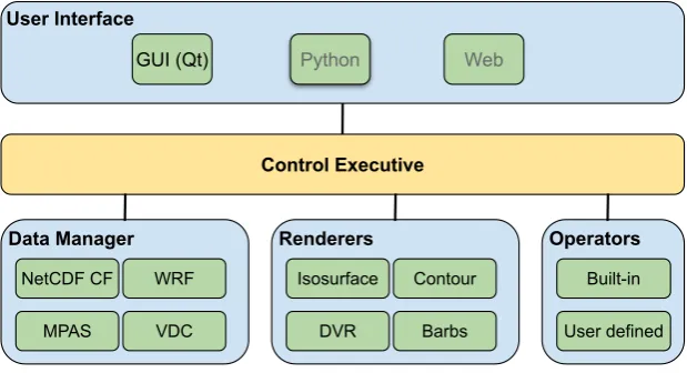
Figure 1.VAPOR software component diagram. The Control Executive marshals data and commands between the User Interface, and the other three primary components: Data Manager, Renderers, and Data Operators.
• Geo-referenced data and image files: VAPOR understands geo-referenced data and is able to 128
combine geo-referenced data from multiple sources: VAPOR can visualize and display them in 129
the scene with correct registration. Moreover, geo-referenced coordinates may undergo mapping 130
projections using a number of supported map projection types. 131
• Vertical coordinate systems: In addition to geo-referenced horizontal coordinates VAPOR 132
supports many of the vertical coordinate systems defined by the CF conventions (e.g. sigma, 133
s-coordinates, and hybrid sigma). 134
• File formats:VAPOR knows how to read many of the file formats and model outputs commonly 135
used in ESS. Most notably VAPOR understands WRF-ARW, MPAS, and CF-compliant NetCDF 136
files. 137
• Grid types: VAPOR supports computational meshes typical of the ESS, such as layered
138
curvilinear grids, layered unstructured grids, and Arakawa grids. Computational intensive 139
visualization algorithms (e.g., direct volume rendering) are also optimized for these grid types. 140
• Missing data: VAPOR understands missing data values that are commonly seen in ESS. For
141
example, in ocean models employing lat-lon grids missing value flags are often used where the 142
computational mesh intersects land masses. 143
3.2. Software Architecture 144
VAPOR is a desktop application implemented in C++. The main software components are 145
depicted in Figure1. Currently, the user interacts with VAPOR though a GUI, which is implemented 146
using Qt: a platform-portable GUI toolkit that enables a common user interface across three major 147
operating systems (macOS, Linux, and Windows). A scripting interface (most likely Python) is planned 148
for the future, as is a web interface. The user interface, whether a GUI or a script, communicates user 149
requests to acontrol executive, which interacts with the remaining three major components of VAPOR: 150
• Data Manager: the component that holds the underlying data, hides file formats and
151
computational grid details, and provides unified data access to the rest of the application; 152
• Operators:a collection of functions that perform calculations on the data prior to rendering; and 153
• Renders: a collection of C++ class objects that implement various 2D and 3D visualization 154
algorithms (e.g., contour lines, isosurfaces, volume rendering, and wind barb plots). 155
3.3. Data Manager 156
The Data Manager is responsible for reading gridded data (heretofore referred to as "variables") 157
metadata, to the rest of the application. The Data Manager presents an abstract representation of 159
gridded data that hides the underlying storage details and to a large degree hides details about the 160
computational grid itself. Clients of the Data Manager, in general, need not be concerned about the 161
grid’s topology (structured or unstructured), geometry (e.g., rectilinear and curvilinear), or VAPOR 162
specific properties (multi-resolution and lossy compression). Other components in the application can 163
query the Data Manager for a list of variable names available in the data collection, the names of the 164
coordinate variables associated with each data variable, the number of time steps present, and so on. In 165
addition to metadata, the Data Manager also satisfies requests to access a named variable at a specific 166
time step and region in space. Variables returned by the Data Manager are not simple arrays of floating 167
point values, but C++ class objects that support a wide variety of operations to facilitate visualization, 168
such as: returning the interpolated value of a point in space, or returning the user coordinates for a 169
node in the mesh. 170
Since analysis and visualization are often I/O bound operations the Data Manager takes 171
steps to minimize I/O costs. Principle among these is to store variables as they are accessed in a 172
memory-resident Least Recently Used (LRU) cache. Subsequent accesses to a variable that is currently 173
in cache will avoid disk reads. The size of the cache is controlled by the user, and may be as large as 174
the operating system of the host platform will allow. 175
Currently the Data Manager is capable of reading a number of commonly used ESS file formats 176
such as CF-compliant NetCDF [25], WRF-ARW [26], MPAS-A [27] and MPAS-O [28]. Additionally, the 177
Data Manager can read VAPOR Data Collection (VDC) with multi-resolution and lossy compression 178
properties. Details of the VDC are discussed in Section4. 179
3.4. Operators 180
VAPOR supports both built-in and user-defined data operators. The former is primarily concerned 181
with transforming mesh coordinate variables. For example, applying projections to map horizontal 182
geographical coordinate systems into “meters-on-the-ground” projected coordinates, or transforming 183
one of the many vertical coordinate systems used in ESS to units of height above (or below) the earth’s 184
surface. In addition to built-in operators VAPOR offers an embedded Python interpreter. Variables 185
may be passed to the interpreter as NumPy arrays, operated on by user-defined Python scripts, and 186
returned to the application as a derived quantity. For example, the user might define a Python script to 187
derive vorticity from the components of velocity. 188
3.5. Renderers 189
VAPOR implements a suite of 2D and 3D visualization algorithms as “renderers,” some of which 190
are very basic (e.g. line contouring), while others are quite advanced (e.g direct volume rendering). 191
In many cases visualization algorithms are comprised of two steps: mapping numerical data into a 192
collection of some form of displayable graphical primitives, and the rendering of those primitives 193
to an image. The latter operation, rendering, is performed using the platform-portable OpenGL 3D 194
rendering library, which is highly optimized for performance and able to take advantage of ubiquitous 195
Graphics Processing Unit (GPU) hardware. While VAPOR is capable of running on systems lacking 196
hardware accelerated graphics, best performance is achieved when some form of hardware graphics 197
acceleration is present. Section5provides more information on the renderers available in VAPOR. 198
3.6. Extensibility 199
VAPOR is an open development package, thus any aspect of the code might be enhanced by the 200
user community. However, the architecture of VAPOR is designed to facilitate three specific forms 201
of extension: 1) addition of new user interfaces; 2) addition of new data readers; and 3) addition 202
(or enhancement) of new (existing) visualization renderers. This goal is achieved via reusable GUI 203
6 of 19
The addition of new GUI elements is facilitated with a collection of composite Qt widgets which 205
implement controls for the most common functionalities of VAPOR. Examples of these controls include 206
variable selectors, transfer function editors, and geometry boundary editors. These composite widgets 207
comprise proper primitive Qt widgets to provide desired controls, and also use consistent layout and 208
size policies to provide a uniform look. The author of a new user interface is then able to reuse these 209
composite widgets in a plug and play fashion. 210
For the addition of new data readers, let us consider a scenario where a new data importer is 211
needed to support a new data format. This is relatively easy with VAPOR’s C++ object-oriented 212
implementation, and involves only deriving a singledata readerclass object from an existinginterface 213
class. An interface class specifies the functions a derived class will need to implement. For example, 214
a data reader derived class must implement a C++ method (function) that returns a list of all of the 215
variable names contained in a data set. Similarly, the derived data reader class will need to implement 216
a function that will read a hyper-slice of data for a specified variable and return the data as an array of 217
floating point values. As a reference, the source file for reading WRF-ARW data is approximately 1,000 218
lines of code. 219
For the addition of new visualization renderers, let us consider a scenario where a new renderer 220
is required to support a novel rendering technique. This is a more complex extension, since it involves 221
both the Renderer and GUI components. The basic steps involve: 1) implementing the actual rendering 222
algorithm, which will operate on data returned from the Data Manager, and producing a rendering by 223
making appropriate calls to OpenGL; and 2) creating the corresponding user interface to expose and 224
control the various rendering parameters required by the new renderer. As with the previous case, in 225
both of these steps the minimally required programming interface is already defined via C++ interface 226
classes, and the implementer need only author the new classes using the interface classes as a recipe. 227
The renderer author will also need to provide a new user interface to support control parameters that 228
are generic (e.g., variable selection) as well as specific to the new renderer. This step again is simplified 229
by making use of the reusable composite Qt widgets. 230
4. VAPOR Data Collection
231
Maintaining interactive performance while visualizing and analyzing high resolution simulation 232
data is a challenging task. Storage capacity, bandwidth, and computational requirements may all limit 233
the rate at which data can be processed and displayed to the screen. One approach for addressing 234
this challenge is the use ofprogressive data access: reduced-size approximations of the data are used for 235
quick-look, exploratory work, and then subsequently refined with more accurate data representations 236
to produce a final rendering or analysis. 237
A straightforward way to support progressive data access that is widely employed by digital 238
mapping technologies such as GoogleMapsTM is multi-resolution: coarsened imagery (data) is 239
transmitted and displayed when the viewpoint is far away, and continuously refined as the user 240
zooms in on a region of interest. 241
Most commonly, multi-resolution representations are simply a hierarchy of approximations 242
created by successively coarsening the original gridded data, reducing the number of grid points along 243
each dimension by a factor of 2 with each pass. There are a number of ways to generate multi-resolution 244
data representations. Sampling the original data points and storing them separately as lower resolution 245
versions is perhaps the simplest one. However, this strategy incurs storage overhead from maintaining 246
separate versions of the data. Space filling curves (e.g., Z-curves [29] and Hilbert curves [30]) offer a 247
way to sample and organize the data without incurring storage overhead. While they do not increase 248
storage, the quality of the coarsened approximations resulting from sampling can be quite poor. 249
A method for achieving higher quality approximations without additional storage is through 250
the use of discrete wavelet transforms [31,32]. Much like discrete Fourier transforms that map data 251
between physical and frequency space, wavelet transforms map data from physical space into a 252
transforms are reversible and exact reconstruction of the original data is possible up to floating point 254
round off error. With a suitable choice of wavelet the number of wavelet coefficients will equal the 255
number of grid points, thus not changing storage requirements. 256
4.1. Wavelet Transforms in VAPOR Data Collection 257
Of interest to our discussion is the multi-resolution properties of wavelets, which permit 258
reconstruction of approximations of the original data at roughly power-of-two grid resolutions, 259
creating a hierarchy of data. Moreover, the reconstructed approximations are weighted averages 260
of neighboring samples, yielding higher quality approximations than sampling. 261
Many wavelets possess another property that is relevant to progressive data access, information 262
compaction, meaning that most of the information contained in a signal (or gridded data set) will be 263
contained in a small subset of the wavelet coefficients. A second form of progressive data access can 264
be realized by ordering the coefficients based on their information content and using only the most 265
important ones for reconstruction. This is often referred to aslossy compression, and similar techniques 266
are widely used in consumer products from JPEG images to streaming audios and videos. 267
Thus two forms of data reduction are possible with wavelets, each, however, with different 268
characteristics. On the one hand, multi-resolution yields a coarsened grid, reducing the computation 269
and memory cost of operations performed on the reconstructed data. On the other hand, lossy 270
compression has no bearing on grid resolution and subsequent costs of operating on the reconstructed 271
data. In other words, there is no benefit to compute or memory bound tasks. 272
VAPOR uses wavelet transforms in its VAPOR Data Collection (VDC) with the support for both 273
forms of progressive data access: multi-resolution and lossy compression. As a result, the VDC enables 274
interactive explorations of very large data with progressive data access. Essentially, the user is afforded 275
the ability to make speed/quality tradeoffs. In practice, VAPOR exposes both multi-resolution and 276
lossy compression controls in the GUI, enabling advanced users to fine tune different combinations of 277
these two parameters based on their knowledge of system bottlenecks. VAPOR also provides a simpler, 278
unified linear “fidelity” control that incorporates both controls ranging from the lowest fidelity (i.e., 279
lowest resolution and maximum lossy compression) to the highest fidelity (i.e., original resolution and 280
no lossy compression). 281
We note that VDC is optional for the users: VAPOR can directly import popular data formats in 282
the ESS field (e.g., WRF and CF-Compliant NetCDF), or convert them to VDC format and then import 283
the VDC files. The conversion tools are packaged and distributed with VAPOR. 284
Finally, the general topic of scientific data reduction is a quite complex and active research area. 285
This survey [33] provides an overview of this topic. 286
4.2. VDC Enabled Workflow 287
The VDC format enables a unique workflow that is suited for data exploration, and follows 288
the Shneiderman’s information visualization mantra: “Overview first, zoom and filter, then 289
details-on-demand” [34]. 290
Using this workflow, the users can start exploring a given large data set at lower fidelity levels. 291
This process can iterate rather rapidly until the user has located areas of interest in space and/or time, 292
selected viewpoints in the case of 3D data, and selected visualization techniques and their parameters 293
such as color maps, isovalues, etc. 294
The user can then increase the fidelity level to examine more details, and keep fine tuning the 295
visualization parameters. Once satisfied with various visualization parameters the user might select 296
the highest data fidelity to render final visualizations at the highest quality for purposes such as 297
publishing or verification of results found with lower fidelity data. 298
8 of 19
Table 1.Test system specifications
CPU: Intel Core-i7 (quad-core, 3.6 GHz) GPU: Nvidia Geforce GTX 1060 Memory: 32 GB
OS: Ubuntu 16.04 To further explore and quantify the benefits of the
300
VDC data format we report a few findings from an 301
evaluation of VDC performance using a commodity 302
computing platform and a relatively large data set. 303
These tests are performed on a Linux desktop with specifications listed in Table1. The test data 304
is one time step of vorticity magnitude from a Taylor Green turbulence simulation [35]. This data 305
set has 32-bit floating point values sampled on a regular grid with a resolution of 1, 0243. Vorticity 306
was chosen for our analysis because it is particularly challenging for any data compression due to the 307
presence of many fine scale structures. 308
4.3.1. Interactivity Improvement 309
Table 2. Frames-per-second on different data resolutions (column) and 3D renderers (row).
Resolution 1283 2563 5123 10243
Volume 25.15 20.88 4.42 0.26 Isosurface 92.86 83.64 27.13 0.27 We first explore benefits to interactivity. When
310
performing data analysis and visualization, interactivity 311
is usually impacted by two operations: reading data from 312
disk (I/O) and rendering (computation). With VDC the 313
former impact is mitigated by both forms of progressive 314
data access, while the latter is solely mitigated by lower 315
resolutions. The I/O impact, however, is difficult to measure in a consistent manner due to complex 316
caching mechanisms baked in to modern operating systems. As a result, here we will only provide 317
measures on the computational impact. 318
We use frames-per-second (FPS) to measure the interactivity, so higher FPS indicates better 319
interactivity. Two computational intensive 3D renderers are tested: direct volume rendering, and 320
isosurface rendering. For each resolution, we use similar rendering parameters so that the resulting 321
renderings look approximately the same, and then test the FPS with those parameters. Table2reports 322
test results, with each frame rate being averaged from twenty test runs. These numbers show that not 323
surprisingly lower resolutions effectively improve interactivity. 324
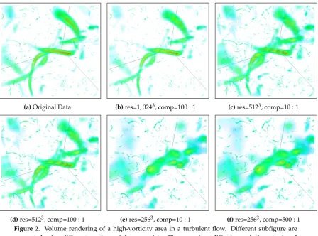
4.3.2. Rendering Quality Impact 325
Multi-resolution representations and lossy compression will of course negatively impact rendering 326
quality. Among these two factors, multi-resolutions have a significantly bigger impact for a given 327
amount of data reduction. We illustrate this impact with different renderings and provide a qualitative 328
evaluation; more quantitative analysis can be found in our previous work [36,37]. 329
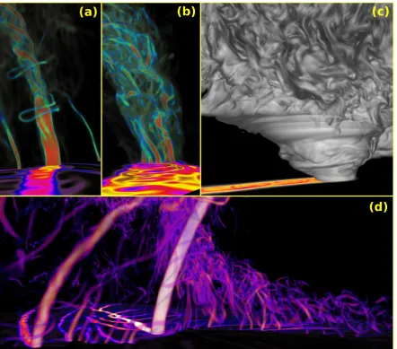
We use volume rendering to visualize the high-vorticity areas, which appear like worms or 330
filaments in a turbulent flow. Figure2highlights one such area that contains a few filaments (in 331
green). Given the original data resolution of 1, 0243, renderings at 5123still can identify and show the 332
basic shapes of filaments, while renderings at 2563lose most details of the identified filaments. These 333
renderings also show results from lossy compression and that lossy compression does not degrade 334
renderings nearly as significantly as lower resolutions. Overall, many of the reduced data renderings 335
still contain sufficient information to establish visualization parameters and perhaps obtain a holistic 336
qualitative understanding of the data. 337
4.3.3. Computational Impact 338
Table 3.Timing of VAPOR to prepare (Prep.) data into VDC format and reconstruct back to gridded data of different resolutions.
Prep. Reconstruct Resolution 10243 10243 5123 2563
Second 107.93 22.11 16.03 15.53 This subsection reports the computational cost
339
of performing wavelet transforms, both forward and 340
inverse. The forward transform is usually performed 341
only once to convert the original data into VDC format, 342
while the inverse transform is performed whenever 343
VAPOR is retrieving data from disk. We remind the 344
reader, however, that VAPOR’s Data Manager is able to 345
(a)Original Data (b)res=1, 0243, comp=100 : 1 (c)res=5123, comp=10 : 1
(d)res=5123, comp=100 : 1 (e)res=2563, comp=10 : 1 (f)res=2563, comp=500 : 1
Figure 2. Volume rendering of a high-vorticity area in a turbulent flow. Different subfigure are generated using different versions of the same data. These versions differ in resolutions (res) and lossy compression ratios (comp), as noted in subcaptions. Subfigure2arepresents the ground truth rendering from the original data.
transforms are performed to prepare all resolution levels, incurring a fixed cost, while the inverse 347
transforms are performed for just enough iterations to retrieve a certain resolution level, incurring a 348
varying cost. Table3reports computational costs for preparing a VDC and reconstructing data from 349
the VDC format. Note that both operations are asymmetric in that reconstruction takes much less time. 350
4.3.4. Storage Impact 351
Table 4.Actual storage size and overhead in percentage of VDC format at different lossy compression ratios. Overhead is compared against the target compression ratio.
Orig. VAPOR Format
Ratio N/A 1:1 10:1 100:1 500:1
Size (MB) 4295 4617.1 751.64 75.17 15.04 Overhead N/A 7.5% 75.0% 75.0% 75.1% Lossy compression allows VAPOR to
352
use either a portion or all of wavelet 353
coefficients to reconstruct anapproximateor 354
faithful version of the original data. This 355
capability, however, requires extra storage 356
for coefficient addressing, resulting the fact 357
that when targeting anX : 1 compression 358
ratio by usingX1 of all coefficients, the actual 359
storage size is more than X1 of the original data size. Table4reports this storage overhead at default 360
compression ratios when converted data is stored in VDC format. 361
5. Visualization Renderers
362
VAPOR provides visualization renderers for both two-dimensional and three-dimensional 363
data. The two-dimensional renderers in VAPOR are similar to corresponding renderers found in 364
batch-processing visualization packages (e.g., NCL); they include: 365
10 of 19
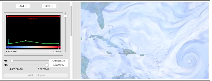
Figure 3.A screenshot of VAPOR. The left panel shows the interface of a transfer function editor, and the right panel shows a visualization of a simulation of 2009’s Hurricane Bill in the Atlantic. The transfer function editor shows a color spectrum of blue to red, and an opacity mapping scheme (in green line segments) with low opacity on both ends of the data range and higher opacity in the middle. The transfer function editor also embeds a data histogram (in cyan) with an obvious spike at the very left. The visualization is a volume rendering of the water vapor content (qvapor) of Bill on top of an image rendering of the earth in the same region. The transfer function specified on the left is applied to the volume rendering (but not image rendering) on the right.
• Barb Renderer:encodes field values as arrows in different directions and lengths; and 367
• 2D Data Renderer:maps data values from a two dimensional variable to different colors. 368
The rest of this section first provides an overview of common visualization controls that enable 369
users to manipulate renderer parameters in VAPOR GUI, and then describes three-dimensional 370
renderers, and the Image Renderer that is unique to VAPOR. 371
5.1. Common Visualization Controls 372
VAPOR’s visualization renderers use different algorithms for image rendering, but they share 373
a set of common controls in the VAPOR application. These common controls are presented using 374
reusable composite Qt widgets as discussed in Section3.6, and their functionalities include selections 375
for variables, VDC data fidelity, geometry boundaries, affine transformations, annotations, and transfer 376
functions, etc. Among the common GUI components, the transfer function editor serves a critical role 377
in data exploration and the creation of informative visualizations, so we describe it in detail. 378
The transfer function editor allows users to define a pair of functions that maps data values 379
to color and opacity, respectively. To adjust color mapping, the user first chooses a color spectrum 380
(either from pre-installed ones or custom designs), and then designates a range of data values to be 381
covered by this color spectrum. To adjust opacity mapping, the user drag-and-drops control points 382
on a sequence of line segments, so the shape of these line segments represents variation of opacity 383
across the designated value range. Data values outside of the designated value range will receive 384
colors and opacity on the range boundaries. After achieving a satisfactory rendering, the user can save 385
the transfer function in a file for future use. 386
The VAPOR transfer function editor further augments user selections by embedding a data 387
histogram in it, so the users are always informed of the relative data frequency of each value, and can 388
assign color and opacity values accordingly. Figure3shows the interface of this widget. 389
5.2. Slice Renderer 390
A Slice Renderer operates on 3D variables. It performs two tasks: 1) extracting a 2D data 391
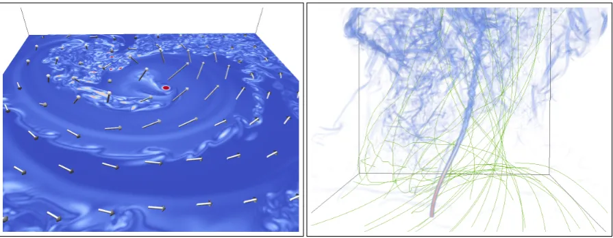
(a)A tomography style slice in perpendicular to the vortex core of a tornado, and a group of barbs showing the wind direction. The slice is of variable cloud liquid water (qcloud), and the barbs are of the wind velocity.
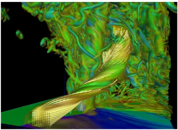
(b) A volume rendering of the vorticy magnitude showing the vortex core of a tornado, and a group of flow lines (in green) of velocity showing trajectories of particles being advected by the tornado.
Figure 4.Showcase of Slice and Barb Renderers (4a), and Volume and Flow Renderers (4b).
user-defined transfer function. The extracted 2D data plane is currently constrained to be aligned to 393
one of the three axes, providing a tomography style examination. Values on the plane are interpolated 394
from the volume using tri-linear interpolation. The Slice Renderer can interactively be positioned 395
and oriented, providing a simple, efficient, and intuitive way to examine volumetric data. Figure4a 396
illustrates a slice rendered perpendicular to the vortex core of a tornado, showing the location of the 397
vortex core in red. 398
5.3. Direct Volume Renderer 399
The Direct Volume Renderer is the flagship renderer for 3D volumetric data. It is useful for both 400
exploring the data as well as close up examination of areas of interest. The Direct Volume Renderer 401
achieves this by enabling the users to “see through” the volume, and by rendering only “interesting” 402
areas in the 3D volume. 403
The Direct Volume Renderer mimics how human sees a semi-transparent 3D object. More 404
specifically, “rays” are emitted from the camera into the 3D volume, just like lines of sight from 405
human eyes. These rays keep traveling inside of the volume, sampling data values along the way, and 406
accumulating colors and opacity at those samples. A ray stops traveling when either 1) it leaves the 407
volume from the back, or 2) it becomes completely opaque after accumulating sufficient opacity. This 408
algorithm is often referred to as “ray casting” in the literature. 409
Using the transfer function editor, users usually assign opacity to only values of interest and leave 410
other values completely transparent, revealing features inside of a 3D volume. Often the renderings 411
resemble natural phenomena, such as a cloud or a tornado. For example, Figure4billustrates a volume 412
rendering of vorticity magnitude from a tornado simulation. With only high vorticity areas being 413
opaque, the vortex core of the tornado is clearly visible. Figure3illustrates a hurricane from volume 414
rendering. More discussion on volume rendering in general can be found in this textbook [38], and its 415
optical models in this paper [39]. 416
VAPOR’s Direct Volume Renderer offers a few noteworthy characteristics: 417
• OpenGL Shading Language (GLSL) implementation. GLSL is a low-level programming
418
interface for Graphics Processing Units (GPUs), which means it’s considerably more performant 419
than higher-level GPU programming paradigms. GLSL is also an open standard and enjoys 420
broad support from all major operating systems and GPU vendors, which means that this high 421
12 of 19
• Separate algorithms optimized for regular and curvilinear grids.VAPOR implements two ray 423
casting algorithms, one for regular and one for curvilinear grids. The algorithm for regular grids 424
takes advantage of the regular grid structure, achieving very high performance. The algorithm 425
for curvilinear grids adapts to the irregular geometry to produce correct renderings at the cost 426
of less performance. To the best of our knowledge, VAPOR is the only visualization package in 427
production use that supports curvilinear grids without expensive and error-prone resampling. 428
• Support for missing values.VAPOR understands missing values that are common in ESS data 429
sets, and does not include them in color and opacity integration during ray casting. 430
• Correct blending with other renderings.The semi-transparency in a volume rendering makes 431
displaying multiple rendering outputs difficult. VAPOR’s Direct Volume Renderer takes into 432
consideration the depth information of other renderings to correctly blend them together, so that 433
the semi-transparent areas of a volume rendering will not block renderings behind it. 434
• Fast rendering mode. Maintaining interactivity requires high rendering performance, usually 435
more than ten frames per second. VAPOR’s Direct Volume Renderer implements a “fast 436
rendering” mode to accommodate this requirement. More specifically, a degraded rendering is 437
producedduringscene navigation (rotation, zoom, etc.), and a normal rendering is produces upon 438
the completion of a sequence (e.g., when the scene rotation finishes). Fast rendering improves 439
overall interactivity for compute intensive operations such as volume rendering. 440
5.4. Isosurface Renderer 441
The Isosurface Renderer displays one or more surfaces in a 3D volume where the field exhibits 442
a user-specified isovalue. Conceptually it is the 3D generalization of 2D contour lines, representing 443
points of a constant value within a region of space. 444
Isosurfaces in VAPOR are computed and rendered using the same basic machinery as direct 445
volume rendering. The only difference is that a ray accumulates opacityonlyat isovalue locations, 446
instead of integrating opacity along the entire ray. Isosurfaces allow examination of the volume in a 447
more quantitative fashion than volume rendering, e.g., when one is interested in a specific data value. 448
Another advantage of isosurfaces is the ability to color map a secondary variable on the isosurface, 449
enabling the examination of two variables simultaneously. Finally, sharing the same code base in GLSL 450
with the Direct Volume Renderer, the Isosurface Renderer has the same portable performance across 451
platforms, flexible algorithm choices for regular and curvilinear grids, and support for fast rendering 452
mode. 453
5.5. Flow Renderer 454
The Flow Renderer performs particle advection, and then renders the resulting trajectories. In 455
the advection step, the user first specifies a three dimensional vector field, which is often velocity or 456
magnetic. The user then specifies particle advection locations in both time and space, along with an 457
advection stopping criterion. VAPOR treats these particles as massless, and uses a Runge-Kutta fourth 458
order method to perform advection on each particle, until the stopping criterion is met. The particle 459
trajectories are rendered in the scene, with optional specifications such as rendering their partial or full 460
lengths, and coloring the trajectories based on a certain property. Figure4billustrates flow rendering 461
in a tornado simulation: particles were placed on the ground, and can be seen to swirl around and 462
move up the tornado. 463
VAPOR’s Flow Renderer supports a number of optional control parameters: 464
• Steady or unsteady fields: The vector field can be steady (constant over time) or unsteady 465
(varying with time) for particle advection. 466
• Seed placement:Starting particle advection locations can be pragmatically determined or be 467
specified by the user using a list of seeding points. When seeds are pragmatically placed, the 468
placement can be uniform or randomly distributed within a user specified region. Moreover, the 469
• Advection direction:For steady fields the particle advection direction can be forward, backward, 471
or bi-directional. 472
• Stopping criteria:The advection can be terminated based on a number of criteria such as leaving 473
the domain, after a specified length of time, etc. 474
• Coloring scheme:Advection trajectories can be colored by different schemes such as another 475
variable or the length of the trajectory. 476
• Save trajectories:Advection trajectories can be saved to a text file with the location and property 477
values at each advection step. 478
5.6. Image Renderer 479
VAPOR can import GeoTIFF raster image files containing geo-referencing information, and 480
display the image in the same coordinate space as any geo-referenced data loaded into the application. 481
The imagery and data will be correctly positioned within the scene. Figure3illustrates a volume 482
rendering of a hurricane on top of a geo-referenced map. VAPOR includes a set of high resolution 483
(500m) global raster image maps from NASA’s Blue Marble Next Generation project [40]. However, 484
any image with proper geo-referencing information can be imported into VAPOR and displayed in the 485
correct location. In fact, the image need not necessarily be a map; data plotted with another tool and 486
stored as a GeoTIFF can be imported just as easily. Finally, with some limitations VAPOR can export 487
the rendered scene as a GeoTIFF that can then be imported into any tool that understands GeoTIFF 488
imagery (e.g., GoogleEarth). 489
6. Use Case
490
6.1. Background 491
VAPOR version two was an invaluable resource for the visualization and analysis of 492
tornado-producing thunderstorms in prior work [41]. Experiences with VAPOR version two in 493
this research has driven some of the refactoring approaches for the VAPOR version three code. Below 494
we present a case study conducted by co-author Orf with VAPOR version three in recent simulations 495
of tornado producing thunderstorms at extremely high resolution. 496
In prior work [41], results from a breakthrough simulation of a violently tornadic supercell was 497
presented. A newly discovered feature dubbed the streamwise vorticity current (SVC) was identified. 498
The SVC is a helical tube of vorticity that begins with a primarily horizontal orientation that, over time, 499
becomes more intense as it is tilted and drawn into the base of a strengthening thunderstorm updraft. 500
The identification of the SVC was made with VAPOR version two utilizing its volume rendering 501
capabilities (see Figure5). The scientific significance of this feature is reflected in the fact that an entire 502
NSF sponsored field program recently was launched to detect it and other similar features in the 503
atmosphere [42]. 504
One of the issues that provided friction for research use of VAPOR version two was the 505
requirement that all data be converted into the VDC format. CM1 output data in this research is 506
saved in HDF5 format, spread amongst many files in a format the authors call LOFS. LOFS data was 507
converted to a series of NetCDF files, each containing several 2D and 3D fields for a given model time. 508
This was followed by the conversion of the NetCDF files to the VDC format, making data import an 509
unwieldy two-step process. 510
6.2. Sources of Data for Current Use Case 511
One of the notable features of VAPOR version three is its ability to natively read CF-compliant 512
NetCDF data [25]. In our current use case, CF-compliant NetCDF files from a thunderstorm simulation 513
are imported directly into VAPOR. In order to create CF-compliant data, modifications to the code 514
that converts LOFS to NetCDF were made in order to provide metadata required by VAPOR, such 515
14 of 19
Figure 5.VAPOR version two volume rendering of the 3D vorticity field and air trajectories calculated using the unsteady flow option from a simulation conducted in year 2014. The tube of vorticity that is embedded with trajectories was dubbed the streamwise vorticity current and is a feature of significant interest in the field of mesoscale meteorology.
to the LOFS conversion code, CF-compliant NetCDF files were created in a single-step process from 517
LOFS data, saving both time and disk space as compared to the two-step process required in previous 518
work. An additional advantage to the current approach is that CF-compliant NetCDF is a standardized 519
format, so a single set of NetCDF files can be natively read by many useful analysis and visualization 520
tools without any further conversions. 521
In the current use case, unprecedented high resolution simulations of a tornado-producing 522
thunderstorm needed to be visualized for presentation at an upcoming conference. The simulation, 523
still unfinished at the time of the conference, utilized most of the Blue Water supercomputer, spanning 524
over 1/4 trillion grid zones. Our goal was to present stills and animations that included the evolution 525
of a devastatingly strong multiple vortex tornado that formed within the simulated thunderstorm. 526
Because the region involving the tornado is a small fraction of the full model domain, NetCDF 527
files spanning only a subdomain were created. The visualization domain for the images shown in 528
Figure6span 501×501×301 grid volumes1. The images in Figure6are a tiny sampling of the 529
total number of images created in this use case. For each of the images shown in this figure, several 530
hundred model times, saved in 1 second intervals, were generated, in order to facilitate the creation of 531
animations. The following process was followed for creating a sequence of images in time: 532
1. Convert the whole LOFS data to disposable NetCDF files containing 2D horizontal data that are 533
then viewed by the slice viewerncviewin order to choose the subdomain bounds desired for the 534
CF-compliant NetCDF files to be input into VAPOR. 535
2. Using the same conversion program, convert LOFS data to CF-compliant NetCDF files spanning 536
the desired subdomain volume. 537
1 The full model simulation mesh contains 11, 200×11, 200×2000 cells, hence the visualization volume contains only 0.03%
16 of 19
3. Launch VAPOR on a Linux workstation, and then import the group of sequentially named 538
NetCDF files. 539
4. Choose from 2D fields the desired surface 2D pseudocolor plot (we chose the vorticity or pressure 540
trace at the surface that shows the path of the tornado and attendant suction vortices that leave a 541
cycloidal path). 542
5. In this use case, volume rendering was used for 3D visualization. For each desired sequence of 543
images, first select the colormap and opacity curves to achieve the desired visualization, and 544
then select the desired camera view. 545
6. Capture a sequence of images to PNG files. During this time, VAPOR steps through each time 546
and visualizes/saves images. This process took roughly one hour per sequence utilizing a 547
Radeon RX 580 graphics card. 548
7. Combine exported PNG files to a MP4 movie. 549
Each image in Figure6represents a different view that highlights features of a simulation that, to 550
our knowledge, contains the highest resolution supercell tornado ever simulated at the time this article 551
was drafted. The presentation of 2D surface swath data in conjunction with volume rendered fields 552
tells a compelling story, especially when animated, showing the path of dozens of subtornadic vortices 553
moving with the storm, some of which converge together towards a central point that ultimately 554
becomes the tornado. Such an information-rich presentation is instantly recognizable by domain 555
scientists including field researchers who study tornadoes, and such visualizations have resulted in 556
calling into question long-standing conceptual models involving tornado formation [43]. Further, 557
carefully crafted volume rendered visualizations involving the cloud and rain fields can easily be 558
compared to photogrammetric observational data of real storms [44,45], validating the numerical 559
model results. 560
7. Discussion and Future Work
561
In this section we discuss some of our our design choices in the development of VAPOR, and lay 562
out our immediate future work. 563
7.1. Design Choice Discussion 564
The software architecture described in Section3is a major design shift over past VAPOR releases, 565
and it has greatly reduced engineering effort and the chance of error during software development. A 566
more detailed discussion was presented in Section3(especially Section3.6); we only summarize here 567
that it has received overwhelmingly positive feedback from the VAPOR development team. 568
The intensive use ofmodernOpenGL and its Shading Language (GLSL) is another big change 569
from past VAPOR releases. While OpenGL has been evolving for more than twenty-five years, its 570
release of version 3.3 has introduced such significant changes that version 3.3 and after are considered 571
modernOpenGL, while versions prior to 3.3 are consideredclassicOpenGL. Among others, one of 572
the most fundamental changes of modern OpenGL is that much of the computation from the classic 573
OpenGL rendering pipeline is now performed byprogrammable shaders, which are written in GLSL and 574
considered much more flexible and powerful. 575
VAPOR migrates its use of OpenGL from classic to modern (from version 2.3 to 4.1). This means 576
we have not only re-written much of the rendering code using GLSL, but also implemented new 577
algorithms that fits the programming model of GLSL (specifically the ray casting algorithm in volume 578
rendering and isosurface rendering). This decision turns out to be a double-edged sword. On the 579
one hand, the more flexible nature of GLSL enables rapid algorithm development and its unique 580
programming model effectively harnesses the massive parallelism on GPUs, delivering very high 581
performance. On the other hand, the reliability of GLSL programs heavily relies on the GPU drivers 582
from GPU vendors, which can vary wildly across operating systems and GPU series. According to our 583
tests, rendering failures are particularly more likely to occur with low-end GPU chips. These failures 584
drivers. However, in the interim these rendering failures directly prompt one of our future work items: 586
the development of CPU-based rendering engines. 587
7.2. Future Work 588
While VAPOR is funded and developed by NCAR, it remains an open-source project on Github 589
(https://github.com/NCAR/VAPOR) and embraces community involvement. This includes user 590
feedback, feature and functionality requests, and direct contributions to the code base. In other words, 591
users have the ability to steer the project. From the perspective of the VAPOR development team, we 592
plan to keep improving VAPOR in the following areas: 593
• More parallelism.VAPOR can benefit from more parallelism in many of its compute intensive 594
calculations. Given the trend of recent parallel computing development, language directive 595
based schemes, such as OpenACC and OpenMP, are probably the best options for VAPOR. 596
• CPU-based rendering engine.We plan to offer a CPU-based rendering engine as an alternative 597
to the current OpenGL based one, hoping to render more reliably on low-end systems. Vendor 598
optimized toolkits, such as OSPRay from Intel, may be a promising candidate. 599
• Dedicated offscreen rendering buffer.Currently VAPOR renders images to a window inside of 600
the application user interface, meaning that the dimension of the final rendering is difficult to 601
specify, and often limited by the monitor size. Dedicating an offscreen rendering buffer would 602
allow bigger and more flexible rendering dimensions. 603
8. Conclusion
604
This paper has provided an overview of the latest iteration of VAPOR (version three), a 605
cross-platform visualization package for data exploration in earth system science. It is a GUI-based 606
desktop application that specifically provides ease of use in the ESS field with support for many 607
numerical models and visualization renderers. Its visualization strength especially lies in the capability 608
to render 3D volumetric data with a Direct Volume Renderer, Isosurface Renderer, and a Flow Renderer. 609
VAPOR also uses various techniques to improve user interactivity, including a hierarchical data 610
organization method and fast rendering modes in compute intensive rendering processes. Version 611
three of VAPOR has improved upon previous releases with a cleaner software architecture, more 612
organized user interface, and the capability to directly operate on computational grids commonly 613
used in ESS. These improvements are aimed at increasing software extensibility and encourage open 614
development from the ESS community. Finally, we demonstrate the usefulness of VAPOR by presenting 615
a use case where VAPOR is used to visualize a simulated tornado and drive scientific discoveries. 616
617
1. Orbach, R.L. Computational Science: A Research Methodology for the 21st Century. APS March Meeting 618
Abstracts, 2004. 619
2. Johnson, C.; Moorhead, R.; Munzner, T.; Pfister, H.; Rheingans, P.; Yoo, T.S. NIH-NSF visualization research 620
challenges report. Institute of Electrical and Electronics Engineers, 2005. 621
3. Childs, H.; Brugger, E.; Whitlock, B.; Meredith, J.; Ahern, S.; Pugmire, D.; Biagas, K.; Miller, M.; Harrison, 622
C.; Weber, G.H.; Krishnan, H.; Fogal, T.; Sanderson, A.; Garth, C.; Bethel, E.W.; Camp, D.; Rübel, O.; Durant, 623
M.; Favre, J.M.; Navrátil, P. VisIt: An End-User Tool For Visualizing and Analyzing Very Large Data. In 624
High Performance Visualization–Enabling Extreme-Scale Scientific Insight; 2012; pp. 357–372. 625
4. Ahrens, J.; Geveci, B.; Law, C. Paraview: An end-user tool for large data visualization. The visualization 626
handbook2005,717. 627
5. Clyne, J.; Rast, M. A prototype discovery environment for analyzing and visualizing terascale turbulent 628
fluid flow simulations. Electronic Imaging 2005. International Society for Optics and Photonics, 2005, pp. 629
284–294. 630
6. Clyne, J.; Mininni, P.; Norton, A.; Rast, M. Interactive desktop analysis of high resolution simulations: 631
18 of 19
7. Upson, C.; Faulhaber, T.; Kamins, D.; Laidlaw, D.; Schlegel, D.; Vroom, J.; Gurwitz, R.; Van Dam, A. The 633
application visualization system: A computational environment for scientific visualization. IEEE Computer 634
Graphics and Applications1989,9, 30–42. 635
8. Schroeder, W.J.; Lorensen, W.E.; Montanaro, G.; Volpe, C.R. VISAGE: an object-oriented scientific 636
visualization system. Proceedings of the 3rd conference on Visualization’92. IEEE Computer Society Press, 637
1992, pp. 219–226. 638
9. Doty, B.; Kinter III, J. Geophysical data analysis and visualization using the Grid Analysis and Display 639
System. Technical report, National Aeronautics and Space Administration, Washington, DC (United 640
States), 1995. 641
10. Schroeder, W.J.; Lorensen, B.; Martin, K.The visualization toolkit: an object-oriented approach to 3D graphics; 642
Kitware, 2004. 643
11. Wald, I.; Johnson, G.; Amstutz, J.; Brownlee, C.; Knoll, A.; Jeffers, J.; Gunther, J.; Navratil, P. OSPRay - A 644
CPU Ray Tracing Framework for Scientific Visualization.IEEE Transactions on Visualization and Computer 645
Graphics2017,23, 931–940. doi:10.1109/TVCG.2016.2599041. 646
12. Nvidia. NVIDIA IndeX: 3D Visualization for Discovery and Exploration. https://developer.nvidia.com/ 647
index. Accessed: 2019-05-23. 648
13. The NCAR Command Language (Version 6.6.2) [Software]. Boulder, Colorado: UCAR/NCAR/CISL/TDD 649
2019. doi:10.5065/D6WD3XH5. 650
14. Williams, D.N.; Doutriaux, C.M.; Drach, R.S.; McCoy, R.B. The flexible Climate Data Analysis Tools (CDAT) 651
for multi-model climate simulation data. 2009 IEEE International Conference on Data Mining Workshops. 652
IEEE, 2009, pp. 254–261. 653
15. May, R.; Arms, S.; Marsh, P.; Bruning, E.; Leeman, J. MetPy: A Python Package for Meteorological Data 654
2008 - 2017. doi:10.5065/D6WW7G29. 655
16. Met Office. Iris: A Python library for analysing and visualising meteorological and oceanographic data sets. Exeter, 656
Devon, v1.2 ed., 2010 - 2013. 657
17. Arendt, A.A.; Hamman, J.; Rocklin, M.; Tan, A.; Fatland, D.R.; Joughin, J.; Gutmann, E.D.; Setiawan, L.; 658
Henderson, S.T. Pangeo: Community tools for analysis of Earth Science Data in the Cloud. AGU Fall 659
Meeting Abstracts, 2018. 660
18. Hoyer, S.; Hamman, J. xarray: ND labeled Arrays and Datasets in Python.Journal of Open Research Software 661
2017,5. 662
19. Rocklin, M. Dask: Parallel computation with blocked algorithms and task scheduling. Proceedings of the 663
14th Python in Science Conference. Citeseer, 2015, number 130-136. 664
20. Hibbard, W.L.; Anderson, J.; Foster, I.; Paul, B.E.; Jacob, R.; Schafer, C.; Tyree, M.K. Exploring coupled 665
atmosphere-ocean models using Vis5D. The International Journal of Supercomputer Applications and High 666
Performance Computing1996,10, 211–222. 667
21. Rautenhaus, M.; Kern, M.; Schäfler, A.; Westermann, R. Three-dimensional visualization of ensemble 668
weather forecasts–Part 1: The visualization tool Met. 3D (version 1.0). Geoscientific Model Development2015, 669
pp. 2329–2353. 670
22. Achtor, T.; Rink, T.; Whittaker, T.; Parker, D.; Santek, D. McIDAS-V: a powerful data analysis 671
and visualization tool for multi and hyperspectral environmental satellite data. Atmospheric and 672
Environmental Remote Sensing Data Processing and Utilization IV: Readiness for GEOSS II. International 673
Society for Optics and Photonics, 2008, Vol. 7085, p. 708509. 674
23. Murray, D.; McWhirter, J.; Wier, S.; Emmerson, S. 13.2 THE INTEGRATED DATA VIEWER–A 675
WEB-ENABLED APPLICATION FOR SCIENTIFIC ANALYSIS AND VISUALIZATION. 19th International 676
Conference on Interactive Information and Processing Systems for Meteorology, Oceanography, and 677
Hydrology, 2003. 678
24. Rautenhaus, M.; Böttinger, M.; Siemen, S.; Hoffman, R.; Kirby, R.M.; Mirzargar, M.; Röber, N.; Westermann, 679
R. Visualization in meteorology—a survey of techniques and tools for data analysis tasks.IEEE transactions 680
on visualization and computer graphics2018,24, 3268–3296. 681
25. Eaton, B.; Gregory, J.; Drach, B.; Taylor, K.; Hankin, S.; Caron, J.; Signell, R.; Bentley, P.; Rappa, G.; Höck, H.; 682
26. Skamarock, W.C.; Klemp, J.B.; Dudhia, J.; Gill, D.O.; Barker, D.M.; Wang, W.; Powers, J.G. A description 684
of the advanced research WRF version 2. Technical report, National Center For Atmospheric Research 685
Boulder Co Mesoscale and Microscale . . . , 2005. 686
27. Skamarock, W.C.; Klemp, J.B.; Duda, M.G.; Fowler, L.D.; Park, S.H.; Ringler, T.D. A multiscale 687
nonhydrostatic atmospheric model using centroidal Voronoi tesselations and C-grid staggering.Monthly 688
Weather Review2012,140, 3090–3105. 689
28. Ringler, T.; Petersen, M.; Higdon, R.L.; Jacobsen, D.; Jones, P.W.; Maltrud, M. A multi-resolution approach 690
to global ocean modeling. Ocean Modelling2013,69, 211–232. 691
29. Morton, G.M. A computer oriented geodetic data base and a new technique in file sequencing; International 692
Business Machines Company New York, 1966. 693
30. Hilbert, D. Ueber die stetige Abbildung einer Line auf ein Flächenstück. Mathematische Annalen1891, 694
38, 459–460. 695
31. Mallat, S.G. A theory for multiresolution signal decomposition: the wavelet representation. IEEE 696
Transactions on Pattern Analysis and Machine Intelligence1989,11, 674–693. 697
32. Strang, G.; Nguyen, T.Wavelets and Filter Banks; Wellesley-Cambridge Press, 1996. 698
33. Li, S.; Marsaglia, N.; Garth, C.; Woodring, J.; Clyne, J.; Childs, H. Data Reduction Techniques for Simulation, 699
Visualization and Data Analysis. Computer Graphics Forum2018,37, 422–447. doi:10.1111/cgf.13336. 700
34. Shneiderman, B. A grander goal: A thousand-fold increase in human capabilities. Educom review1997, 701
32, 4 – 10. 702
35. Mininni, P.D.; Gómez, D.O.; Mahajan, S.M. Direct simulations of helical hall-mhd turbulence and dynamo 703
action.The Astrophysical Journal2005,619, 1019. 704
36. Li, S.; Gruchalla, K.; Potter, K.; Clyne, J.; Childs, H. Evaluating the Efficacy of Wavelet Configurations on 705
Turbulent-Flow Data. Proceedings of IEEE Symposium on Large Data Analysis and Visualization; , 2015; 706
pp. 81–89. doi:10.1109/LDAV.2015.7348075. 707
37. Li, S.; Sane, S.; Orf, L.; Mininni, P.; Clyne, J.; Childs, H. Spatiotemporal Wavelet Compression for 708
Visualization of Scientific Simulation Data. 2017 IEEE International Conference on Cluster Computing 709
(CLUSTER), 2017, pp. 216–227. doi:10.1109/CLUSTER.2017.15. 710
38. Lichtenbelt, B.; Crane, R.; Naqvi, S. Introduction to Volume Rendering; Prentice-Hall, Inc.: Upper Saddle 711
River, NJ, USA, 1998. 712
39. Max, N. Optical models for direct volume rendering. IEEE Transactions on Visualization and Computer 713
Graphics1995,1, 99–108. doi:10.1109/2945.468400. 714
40. Stöckli, R.; Vermote, E.; Saleous, N.; Simmon, R.; Herring, D. The Blue Marble Next Generation-A true 715
color earth dataset including seasonal dynamics from MODIS.Published by the NASA Earth Observatory 716
2005. 717
41. Orf, L.; Wilhelmson, R.; Lee, B.; Finley, C.; Houston, A. Evolution of a Long-Track Violent Tornado within 718
a Simulated Supercell. Bull. Am. Meteorol. Soc.2017,98, 45–68. doi:10.1175/BAMS-D-15-00073.1. 719
42. Tracking a supercell thunderstorm across the Great Plains.https://www.nsf.gov/discoveries/disc_summ. 720
jsp?cntn_id=298179. Accessed: 2019-07-15. 721
43. Orf, L. Petascale supercell thunderstorm simulations and a new hypothesis for tornado formation and 722
maintenance. https://youtu.be/5cel1fLxR04?t=2674, 2019. Presented at the CSME-CFDSC Congress, 723
London, ONT. 724
44. Schyma, H.; Orf, L. Science inside a tornado - Decoding the EF5.https://youtu.be/e2wbn3ivHwc?t=646, 725
2019. Video documentary. 726
45. Schyma, H.; Orf, L. Tornado science & super computers - Tornado footage compared with simulations. 727