Sum-of-Squares Meets Program Obfuscation,
Revisited
Boaz Barak?, Samuel B. Hopkins??, Aayush Jain? ? ?, Pravesh Kothari†, and Amit Sahai‡.
Abstract We develop attacks on the security of variants of pseudo-random generators computed by quadratic polynomials. In particular we give a general condition for breaking the one-way property of map-pings where every output is a quadratic polynomial (over the reals) of the input. As a corollary, we break the degree-2 candidates for security assumptions recently proposed for constructing indistinguishability ob-fuscation by Ananth, Jain and Sahai (ePrint 2018) and Agrawal (ePrint 2018). We present conjectures that would imply our attacks extend to a wider variety of instances, and in particular offer experimental evidence that they break assumption of Lin-Matt (ePrint 2018).
Our algorithms use semidefinite programming, and in particular, results on low-rank recovery (Recht, Fazel, Parrilo 2007) and matrix completion (Gross 2009).
?Harvard University.[email protected].
?? University of California, Berkeley.[email protected]. ? ? ? University of California, Los Angeles.[email protected].
†
Princeton University and the Institute for Advanced [email protected]. edu.
‡
1
Introduction
In this work, we initiate the algorithmic study of cryptographic hardness that may exist in general expanding families of low-degree polynomials over R. As
a result, we obtain strong attacks on certain pseudorandom generators whose output is a “simple” function of the input. Such “simple” pseudorandom gener-ators are interesting in their own right, but have recently become particularly important because of their role in candidate constructions forIndistinguishabily Obfuscators.
The question of whether Indistinguishabily Obfuscators (iO) exist is one of the most consequential open questions in cryptography. On one hand, a sequence of works [14,29] has shown that iO, if it exists, would imply a huge variety of cryptographic objects, several of which we know of no other way to achieve. On the other hand, the current candidate constructions for iO’s are not based on well-studied standard assumptions, and there have been several attacks on several iO constructions as well as underlying primitives.
A promising line of works [19,23,3,20,22] has aimed at basing iOs on more standard assumptions, and in particular Lin and Tessaro [22] reduced construct-ing iO to the combination followconstruct-ing three assumptions:
1. Thelearning with errors (LWE) assumption.
2. Existence of three local pseudorandom generators with sufficiently large super linear stretch. These are pseudorandom generators G : {0,1}n → {0,1}n1+ε (for arbitrarily smallε >0) such that if we think of the input as split inton/kblocks of lengthkeach (for somek=no(1)) then every output
ofGdepends on at most three blocks of the input.
3. Existence oftrilinear mapssatisfying certain strengthening of the Decisional-Diffie-Hellman assumption.
Of the three assumptions, the learning with errors assumption is well studied and widely believed. The existence of local pseudorandom generators has also been recently extensively studied; it also relates to questions on random con-straint satisfaction problems that have been looked at by various communities. Based on our current knowledge, it is reasonable to assume that such three-local generators exist with stretch, say, n1.1 which would be sufficient for the
Lin-Tessaro construction.
k= 2 orbilinear case, where we have had constructions for almost 20 years that are believed to be secure (with respect to classical polynomial-time algorithms) based on elliptic curve groups that admit certainpairing operations [5]. Thus a main open question has been whether one can achieve iO based only on cryp-tographic bilinear maps as well as local (or otherwise “simple”) pseudorandom generators that can be reasonably conjectured to be secure.
1.1 Basing iO on bilinear maps and our results
In the first version of their manuscript, Lin and Tessaro [22] gave a construction of iO based ontwo local generators with a certain stretch, and a candidate con-struction for the latter object based on a random two-local map with a certain nonlinear predicate. Alas, Barak, Brakerski, Komargodski and Kothari, [4], as well as Lombardi and Vaikuntanathan [24] showed that the Lin-Tessaro candi-date construction, as well asany generator with their required parameters, can be broken using semidefinite programming, and specifically the degree two sum of squares program [4].
Very recently, the work of Ananth, Jain, and Sahai [2], followed shortly by the independent works of Agrawal [1] and Lin and Matt [21], proposed a way around that hurdle, obtaining constructions for iO where the role of the trilinear map is replaced with objects that:
1. Satisfy security notions that are weaker than being a full fledged pseudoran-dom generators.
2. Satisfy structural properties that are weaker than being two-local, and in particular requiring the outputs only to be adegree two1 polynomial of the
input.
As such, these objects do not automatically fall under the attacks described by [4,24]. However, in this work we show that:
– The specific candidate objects in all these three works (based on random polynomials) can be broken using a distinguisher built on the same sum-of-squares semidefinite program.
– Moreover, this results extends to other families of constructions, including ones that are not based on random polynomials. In fact, we do not know of
any degree-2 construction that does not fall prey to a variant of the same attack.
1
The Ananth-Jain-Sahai “Cubic Assumption”. The work of [2] also obtained a construction of iO based on a (variant of a) pseudorandom generator where every output is a cubic polynomial of the input, but where some information about the input is “leaked” in a way “masked” using instances of LWE2. Our attacks in their current form are not applicable to this new construction. The question of whether secure degree-3∆RGs exist, or whether an extended form of the sum of squares algorithm can be applied to it, is one that deserves further study. More generally, understanding the structure of hard distributions for expanding families of constant-degree polynomials over the integers, is a fascinating and important area of study, which is strongly motivated by the problem of securely constructing iO. Taking inspiration from SoS lower bounds [15,30], we also sug-gest a candidate for the same. Our candidate is inspired by the hardness of refuting random satisfiable 3SAT instances. For further details, see Section7.
1.2 Our Results
We consider the following general hypothesis that, if true, would rule out not just the three proposed approaches based on quadratic polynomials for obtaining iO, but also a great many potential generalizations of them. Below we say that an n-variate polynomial q is Λ-bounded if all of q’s coefficients are integers in the interval [−Λ,+Λ]. We say that a distributionX over Zn is Λ bounded if it
is supported over [−Λ,+Λ]n.
Hypothesis 1 (No expanding weak quadratic pseudorandom genera-tors).For every ε >0, polynomialΛ(n), sufficiently large n∈N, if:
– q1, . . . , qm:Rn →Rare quadraticΛ(n)-bounded polynomials for m>n1+ε
– X is aΛ(n)-bounded distribution overZn
– For everyi,∆i is aΛ(n)bounded distribution overZsuch thatP[∆i =z]<
0.9 for everyz∈Z.
then there exists an algorithmA that can distinguish between the following distributions with Ω(1)bias:
– (q1, . . . , qm, q1(x), . . . , qm(x))forx∼ X.
– (q1, . . . , qm, q1(x) +δ1, . . . , qm(x) +δm)where for every i,δi is drawn
inde-pendently from∆i.
Note that this hypothesis would be violated by the existence of a pseudoran-dom generatorG:{0,1}n→ {0,1}n1+ε whose outputs are degree two polynomi-als. It would also be violated if the distribution G(x) is indistinguishable from
2
the distribution (G(x) +δ10, . . . , G(x) +δ0m) whereδ01, . . . , δm0 are drawn indepen-dently from some distribution∆over integers that satisfiesP[∆= 0]60.9.
An efficient algorithm to recoverxfromq1(x), . . . , qm(x) would allow to
dis-tinguish between the two distributions. However, generally speaking, it need not even be information theoretically possible to recover x from this information. Even if it is information-theoretically possible this can be computationally in-tractable, as recovering x from q1(x), . . . , qm(x) is an instance of the NP hard
problem ofQuadratic Equations.
In Hypothesis1, the polynomials are arbitrary. However, the candidate con-structions of pseudorandom generators considered so far usedq1, . . . , qmthat are
sampledindependently from some distributionQ. This is natural, as intuitively if we want q1(x), . . . , qm(x) to look like a product distribution, then the more randomness in the choice of theqi’s the better.
However, in this work we give general attacks on candidates that have this form. As these are some of the most natural approaches to refute Hypothesis1, our work can be seen as providing some (partial) evidence to its veracity. To state our result, we need the following definition of “nice” distributions.
Definition 1 (Nice distributions). Let Q be a distribution over n-variate quadratic polynomials with integer coefficients. We say that Qis niceif it satis-fies that:
– There is a constant C = C(Q) = O(1) such that Q is supported on ho-mogeneous(i.e. having no linear term) degree-2 polynomials q with kqk2
26
CEkqk2
2, wherekqk is the`2-norm of the vector of coefficients ofq.
– V ar(Qi,j) = 1 where Qi,j denotes the coefficient of xixj in a polynomialQ
sampled fromQ.
– If{i, j} 6={k, `}then the random variables Qi,j andQk,` are independent Roughly speaking, a distribution over quadratic polynomials is nice if it sat-isfies certain normalization properties as well as pairwise independence of the vectors of coefficients. Many natural distributions on polynomials are nice, and in particular random dense as well as random sparse polynomials are nice.
The following theorem shows that it is always possible to recoverxfrom a superlinear number of quadratic observations, if the latter are chosen from a nice distribution.
Theorem 2 (Recover from random quadratic observations). There is a polynomial-time algorithm A (based on the sum of squares algorithm) with the following guarantees. For every nice distribution Q and every t 6 nO(1), for large-enough n, with probability at least 1 − n−log(n) over x ∼ {−t,−t+ 1, . . . ,0, . . . , t−1, t}n andq
On “niceness”. The definition of “nice” distributions above is fairly natural, and captures examples such as when the polynomials are chosen with all coefficients as independent Gaussian or Bernoulli variables. In particular as a corollary of Theorem2we break the candidate pseudorandom generator of Ananth et al (and even its ∆-RG property). Moreover, we obtain such results even in the sparse
case where most of the coefficients of the polynomialsq1, . . . , qmare zero.
At the moment however our theoretical analysis does not extend to the “blockwise random” polynomials that were used by Lin and Matt which can be thought of as a sum of random dense polynomial and a random sparse poly-nomial. While this combination creates theoretical difficulty in the analysis, we believe that it can be overcome and that it is possible to recover in this case as well. In particular, we also haveexperimental resultsshowing that we can break the Lin-Matt generator as well.
Finally, we note that by Markov’s inequality for any Q we haveP(kqk2 >
CEkqk2)
61/C. Our niceness assumption just has the effect of restrictingQto this relatively high-probability event. IfQis not pathological – that is, it is not dominated by events with probability1/C for a large constantC – then this kind of truncation will result in a nice distribution.3
On the distribution of x. For concreteness, we phrase Theorem 2 so that the distribution of x is uniform over {−t, . . . , t}n. However, the proof of the theo-rem allowsxto be a more general Rn-valued random variable. In particular,x
may be anyn-dimensional real-valued random vector which hasEx= 0 and is
O(Ekxk2/n)-sub-Gaussian. The coordinates ofxneed not even be independent:
for instance,xmay be drawn from the uniform distribution on the unit sphere.
Experiments. We implement the sum-of-squares attack and verify that indeed it efficiently breaks random dense quadratic polynomials. Furthermore, we im-plement a variant of the attack that efficiently breaks the Lin-Matt candidate:
3
Along the same lines, we note that ifQis nice andEq∼Qq= 0 (as we observe later,
the latter can be enforced without loss of generality) thenQis alsoΛ(n)-bounded forΛ(n)6O(n). The reason is that ifQis nice and hasEq= 0 then
Ekqk2=
X
i,j6n
EQ2ij= X
i,j6n
V ar(Qij) =n2.
For every i, j and every q in the support of Q, we have by niceness that |qij| 6 kqk26Cn. HenceQisO(n)-bounded.
One implication is thatQcannot be a distribution on where the all-zero polyno-mial appears with probability, say, 1−1/n, as otherwise its support would also have to contain polynomials with coefficients n. Our main theorem could not apply to such a distribution, since clearly at least Ω(n2) independent samples would be needed to get enough information to recover x from {qi, qi(x)}, while we assume
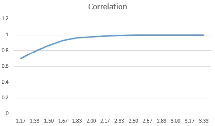
the Lin-Matt candidate is, roughly speaking, a sum of two independent poly-nomials, where one is dense and one is sparse. Since the planted solution must be composed of polynomially-bounded integers, we observe that it is possible to efficiently guess the squared L2 norm of the portion of the planted solution that corresponds to the sparse part of the polynomial. Given this guess, we can introduce a new constraint into the semidefinite program that fixes the trace of the portion of the semidefinite matrix that corresponds to the sparse matrix. We show experimentally that this attack breaks the Lin-Matt candidate for moder-ate values of n. In particular, in Figure 1 we plot the correlation between the recovered solution with the planted solution, where the x-axis is labeled by the ratiom/nshowing the expansion needed for the attack to work, forn= 60 total variables. More details can be found in Section6.
In particular, we are not aware of any candidate construction of weak pseu-dorandom generator computed by quadratic polynomials that is not broken ex-perimentally by our algorithms.
Figure 1: Experimentally breaking Lin-Matt candidate. Graph shows quality of recov-ered solution vs. planted solution, for various values ofm/nshown in the x-axis. Let vbe the eigen vector with largest eigen value of the optimum matrix returned by the SDP. Letxbe the planted solution. Quality of solution is defined as hv,xi
2
Our techniques
Our algorithms use essentially the same semidefinite program constraints that were used in the work of [4], namely the sum of squares program. However, we use a different, simpler, objective function, and moreover we crucially use a different analysis (which also inspired some tweaks to the algorithm that seem to help in experiments). Specifically, consider the task of recovering an unknown vectorx∈Rn from the values (q1(x), . . . , qm(x)) whereq1, . . . , qmare quadratic polynomials. We focus on the case that the qi’s are homogenous polynomials, which means that (thinking of xas a column vector),qi(x) = x>Qixfor some n×nmatrixQi. Another way to write this is thatqi(x) =hQi, XiwhereX is the rank one matrixxx>.
In the above notation, our problem becomes the task of recovering a rank one matrixX from the observations
hQ1, Xi, . . . ,hQm, Xi (2.1)
for some knownn×nmatricesQ1, . . . , Qmwherem>n1+ε. Luckily, this task
has been studied in the literature and is known as the low rank recovery prob-lem [28]. This can be thought of as a matrix version of the well known problem of sparse recovery (a.k.a.compressed sensing) of recovering an k-sparse sparse vector x∈Rn (forn k) from linear observations of the form A1x, . . . , Ak0x
wherek0 is not much bigger thank.
While the low rank recovery problem is NP hard in the worst-case, for many inputs of interest it can be solved by a semidefinite program minimizing the
nuclear norm of a matrix. This semidefinite program can be thought of as the matrix analog of the L1 minimization linear program used to solve the sparse
recovery problem. In particular, it was shown by Recht, Fazel and Parrilo [28] that if theQi’s are random (with each entry independently chosen from, say, a random Gaussian or Bernoulli distribution), then they would satisfy a condition known asmatrix restricted isoperimetry property (matrix RIP)that ensures that the semidefinite matrix recoversX in our regime of m>n1+ε.
This already rules out certain candidates, but more general candidates have been considered. In particular, the results of Recht et al are not applicable when the Qi’s are sparse random matrices, which have been used in some of the iO constructions such Lin-Matt’s. Luckily, this problem has been studied by the optimization community as well. The extremely sparse case, where each of the Qi’s has just a single nonzero coordinate, is particularly well studied. In this case, recovering X from (2.1) corresponds tocompleting X using m observations of its entries, and is known as thematrix completion problem.
showed that it is possible to recover X from (2.1) as long as these observations Q1, . . . , Qmare sampled independently from a collection{Q1, . . . , QN}that
sat-isfies certain “isotropy” and “incoherence with respect to X” properties. We show that under the “niceness” conditions of Theorem2, we can “massage” our input so that it is of the form where Gross’s theorem applies. Once we do so we can appeal to this theorem to obtain our result. A key property that we use in our proof is that in the cryptographic setting, we do not need to recover X = xx> for every x ∈
Zn but rather only for most x’s. This allows us to
achieve the incoherence property even in settings where it would not hold for a worst-case choice of a vector.
3
Preliminaries
For a matrix X, we write kXk for its operator norm: supv:kvk2=1|hv, Xvi. We use the standard inner product on the Hilbert space of n×n matrices: hA, Bi = tr(AB). The nuclear norm of a matrix X is defined by kXk∗ = supA:kAk61hA, Xi. For a positive semidefinite matrixX, kXk∗= tr(X).
For any matrixQ∈Rn×n, vec(Q) denotes “vectorization” of the matrix Q
as an2 dimensional vector.
For a matrixM ∈Rn×n, we define the operator norm (also called the spectral norm) of M as maxx∈RnkM xk/kxk. The Frobenius norm of M is kMkF =
q P
ij6nMij2.
For a matrixM, we writeM ∈(1±ε) Id ifkM−Idk6ε, wherek · kis the operator norm.
3.1 ∆RGs (Ananth-Jain-Sahai)
Ananth-Jain-Sahai proposed a variant of (integer valued) PRG such that it is hard to distinguish between the output of a PRG and a small perturbation of it. Specifically, the following definition describes the object they proposed.
Definition 2 ((n, λ, B, χ)-∆RG). Let f :χn →
Zm be an integer valued
func-tion with theith output described byfi :χn →Zand at anyx∈χn,fi(x) =qi(x)
for quadratic polynomialsqi for16i6m.
f is said to be a ∆RG, if for distributionsD1, D2 on Zm defined below and
for any circuitA of size2λ, | P
z∼D1
[A(z) = 1]− P z∼D2
[A(z) = 1]|<1−2/λ
Distribution D1
Distribution D2
Samplex←χ. Output {qi, qi(x) +δi}i∈[m]
Here δi∈Zare arbitrary perturbations such that |δi|< B for alli∈[m].
Concurrently and independently, [21] proposed Pseudo-Flawed Smudging Generators which have similar security guarantees.
4
Candidates for Quadratic PRGs
In this section we formally describe the candidate polynomial and input distri-butions proposed by [2,21,1] to realize corresponding notions of pseudo-random generators of Z.
Note that any algorithm that given the polynomialsq1, . . . , qmand measure-mentsq1(x), . . . qm(x) whenx,q1, .., qmare sampled from required distributions
of the pseudorandom generator, successfully recovers x, also breaks the corre-sponding candidate for the pseudorandom generator.
To be precise, we describe the candidate polynomials and input distributions proposed by:
– Ananth et al. [2] to instantiate∆RGs.
– Lin-Matt [21] to instantiate Pseudo Flawed-Smudging Generators.
– Agarwal [1] to instantiate Non-boolean PRGs.
Along with assumptions on cryptographic bilinear maps, learning with error assumption and PRGs with constant block locality, either of these three as-sumptions imply iO.
4.1 Candidate for ∆RG
Ananth-Jain-Sahai proposed the following candidate construction for a ∆RG. Let χ be the uniform distribution in [−B1, B1]. Choose m = n1+ε for some
small enough constant ε >0. Let C be some constant positive integer and B1
be a polynomial in λ, the security parameter.
Distribution Q: Sample each polynomial as follows. Let q(x1, ..., xn) = Σi6=jci,j·xi·xj, where each coefficientci,j is chosen uniformly from [−C, C].
4.2 Candidate for Pseudo Flawed-Smudging Generators (Lin-Matt)
Lin and Matt [21] proposed a variant of pseudorandom generators with security properties closely related to the notion of ∆RGs above. Here, we recall their candidate polynomials.
DistributionQ: For eachj ∈[m],
qj(x1, ..., xn, x01, ..., x0n0) =Sj(x1, ..., xn) +M Qj(x01, ..., x0n0)
Here we write more about polynomialsSj, M Qj.
1. M Qj Polynomials: M Qj are random quadratic polynomials over (x01, ..., x0n0), where the coefficients of each degree two monomial x0ix0k and
degree one monomialx0i are integers chosen independently at random from [−C, C].
2. Sj Polynomials:Sj are random quadratic polynomials over (x1, ..., xn) of
the form:
Sj(x1, ..., xn) =Σ
n/2
i=1αixσj(2·i)xσj(2·i−1)+Σ n
i=1βixi+γ
Here each coefficientαi,βiandγare random integers chosen independently from [−C, C]. Here,σj is a random permutation from [n] to [n].
DistributionX:
1. Eachxifori∈[n] is chosen as a random integer sampled independently from the distribution χB1,B2. χB1,B2 samples a random integer from [−B1, B1] with probability 0.5 and from [−B2, B2] with probability 0.5.
2. Distribution of inputsx01, ..., x0n0:Each x0i is chosen as a random integer
sampled independently from the distribution χB0. χB0 samples a random
integer from [−B0, B0].
Parameters:SetB1, B2, B0, n, n0 as follows:
– Setn=n0 andm=n1+ε, for someε >0. – B1,B0 andC are set arbritarily.
– SetB2=Ω(nB2+nBB1).
HereB is some polynomial in the security parameter.
All the pseudorandom generators we consider are maps from Zn into Zm
where each of themoutput is computed by a degree 2 polynomial with integer coefficients in the input. Since any degree two polynomial in Rn can be seen as a linear map onRn×n4, one can equivalently think of such PRGs as linearly
mapping symmetric rank 1 matrices into Rm.
4
For any q(x) = P
i,jqi6jxixj, we define Q: Rn×n →R byQi,j = Qj,i = qi,j/2.
5
Inverting Linear Matrix Maps
In this section, we describe the main technical tool that we rely on in this work - an algorithm based on semidefinite programming for inverting linear matrix maps.
Definition 3 (Linear Matrix Maps). A linear matrix map A:Rn×n →Rm
described by a collection of n×n matricesQ1, Q2, . . . , Qm is a linear map that
maps any matrix X ∈ Rn×n to the vector A(X) ∈
Rm such that A(X)i = hQi, Xi.
We will use calligraphic letters such asAandBto denote such maps.
We are interested in the algorithmic problem ofinvertingsuch maps, that is, finding X given A(X). IfQis are linearly independent and mn2, then this can be done by linear equation solvers. Our interest is in inverting such maps for low rank matrices X with the “number of measurements” mn2. Indeed, our results will show that for various classes of linear mapsA, we can efficiently find a low-rank solution toA(X) =z, whenever it exists, form= ˜O(n).
Such problems have been well-studied in the literature and rely on a primitive based on semidefinite programming called “nuclear norm minimization”. We will use this algorithm and rely on various known results about the success of this algorithm in our analysis.
Algorithm 3 (Trace Norm Minimization).
Given: – Adescribed byQ1, Q2, . . . , Qm∈Rn×n.
– z∈Rm.
Operation: Output X= arg min X0
A(X)=z tr(X).
In what follows, we will give an analysis of this algorithm for a class of linear matrix maps.
5.1 Incoherent Linear Measurements
In this section we describe a remarkably general result due to Gross on a class of instancesx, Q1, . . . , Qmfor which trace norm minimization recoversx[16]. These
instances are calledincoherent. Gross’s result is the main tool in the proof of our main theorem, which will ultimately show that “nice” distributionsQ produce incoherent instances of trace norm minimization.
we would like to apply our main theorem – for example, if Q1, . . . , Qm have independent entries with on average 1 nonzero entry per row.
Definition 4 (Incoherent Overcomplete Basis).LetB={B1, B2, . . . , BN}
be a collection of matrices in Rn×n. For any rank 1 matrix X ∈ Rn×n , B is
said to be ν-incoherent basis for X if the following holds:
1. (1−o(1))1/n2I
n2×n2 1/NPNi=1vec(Bi)vec(Bi)> (1 +o(1))1/n2In2×n2.
2. For eachi6N,|hX, Bii|6ν/n· kXkF. We can now define aν-incoherent measurement.
Definition 5 (Incoherent Measurement).LetBbe aν-incoherent overcom-plete basis for an n×nrank 1 matrix X, and supposeB has size N= poly(n). Let A: Rn×n →Rm be a map obtained by choosing Qi for eachi6m to be a
uniformly random and independently chosen element of B. Then, A is said to be aν-incoherent measurement ofX.
The following result follows directly from the Proof of Theorem 3 in the work of Gross [16]. While that work focuses onBbeing orthonormal - the proof extends to approximately orthonormal basis (i.e., part 1 in the above definition) in a straightforward way.
Theorem 4. Let B be a ν-incoherent basis for a rank 1 matrix X of size N = poly(n). Let A:Rn×n →Rm be a map obtained by choosingQi for eachi6m
to be a uniformly random and independently chosen element of B. Then, for large enoughm=Θ(νnpoly logn), Algorithm 3, when given inputAandA(X)
recoversX, with probability at least1−n−10 log(n) over the choice of A.
5.2 Invertible Linear Matrix Maps
In this section we prove Theorem2 on solving random quadratic systems.
Proof (Proof of Theorem2).Fixt6nO(1) and a nice distributionQ.
CenteringWe may assume thatEQQ= 0. Otherwise, we can replaceQwith Q0 whereQ0 =√1
2(Q0−Q1) for independent drawsQ0, Q1∼ Q. This is because
Q0 remains nice ifQis, clearly
EQ0 = 0, and givenq1, . . . , qm, q1(x), . . . , qm(x)
our algorithm can pairito i+ 1 (for eveni) and instead considerm/2 samples of the form (1/√2)(qi+qi+1),(1/
√
2)(qi(x) +qi+1(x)). Thus for the remainder
of the proof we assume EQ= 0.
Our goal is to establish that there isN 6nO(1) such that ifQ1, . . . , QN are
Incoherence part one: orthogonal basisFirst observe that sinceEQ= 0 andEQ2ij = 1 and our pairwise independence assumption, we have
Evec(Q)vec(Q)>= Idn2×n2 .
Also, by niceness, every |Qij| 6 O(n) with probability 1, for every i, j. Fix i, j, k, ` 6 n. By the Bernstein inequality, given N independent draws Q(1), . . . , Q(N), for anys
>0, P 1 N X
a6N
Q(ija)Q(k`a)−EQijQk` > s 6exp
−CN s2
n4+sn2
for some universal constantC. Takes= 1/n4 and N =n10, this probability is at most exp(−O(n2)). Taking a union bound over i, j, k, ` ∈ [n], we find that
with probability at least 1−exp(−O(n2)),
(1−o(1)) Idn2×n2 1 N
X
a6N
vec(Q(a))vec(Q(a))> (1 +o(1)) Idn2×n2 .
Incoherence part two: small inner productsNext we establish the other part of incoherence: that n12hx, Q(a)xi6ν/nfor alla6N. The coordinates of the vectorxare independent, and each is bounded byt. Thusxis sub-Gaussian, with variance proxy O(t2). Since the coordinates of x have
Ex2i > Ω(t2), the random vectory with coordinatesxi/pEx2i has sub-Gaussian normO(1).
Consider a fixed matrixM ∈ Rn×n, where M has Frobenius norm kMkF
and spectral normkMk. By the Hansen-Wright inequality, for anys>0,
P
y
|y>M y−Ey>M y|> s 6exp −Cs2/(kMk2F+skMk
for some constantC.
IfQ is any matrix in the support of Q, then kQ/nkF 6 O(1) by niceness, andkQk6kQkF. So for any suchQ,
P
y
|y>(Q/n)y−Ey>(Q/n)y|> s 6exp −Cs2/(1 +O(s)).
Taking s = (logn)4, this probability is at most n−(logn)2 for large-enough n.
Taking a union bound over N 6nO(1) samplesQ(a), with probability at least
1−n−(logn)1.5 overy (for large enoughn), everyQ(a) has
x>·Q
(a)
n ·x 6
(logn)O(1) n · kxx
>kF.
Putting it together, forN =nO(1), with probability at least 1−n−(logn)1.4 for big-enoughn, ifx∼ {−t, . . . , t}n thenQ(1)/n, . . . , Q(N)/n are a (logn)O(1)
Q(1), . . . , Q(N), we have
Px(Q(1)/n, . . . , Q(N)/nisν-incoherent forx) > 1 − n−10 logn (again for large enoughn).
From incoherence to recoveryWe can simulate the procedure of sampling Q1, . . . , Qm as in the theorem statement by first sampling Q1, . . . , QN, then
randomly subsamplingmof theQ’s. IfQ1, . . . , QN are (logn)O(1)-incoherent for xx>, then Theorem 4 shows that with probability 1−n−logn over the second sampling step, trace norm minimization recovers x, so long as the number of samplesmis at leastn(logn)O(1). This finishes the proof.
6
Experiments
In this section, we describe the experiments that we performed on various classes of polynomials and how well do they perform in practice. All the codes were run and analysed on a MacBook Air (2013) laptop with 4GB 1600 Mhz DDR3 RAM and an intel i5 processor with clock speed of 1.3 Ghz. We used Julia as our programming language and the package “Mosek” for the implementation of an SDP solver.
6.1 Experimental Cryptanalysis of Dense or Sparse Polynomials
First, we describe the setting of multivariate quadratic polynomials over the integers where the coefficients of each monomial is chosen independently at ran-dom from some distributionD. Such dense polynomials were considered in [2,1]. We denote such polynomials by M Q.
The functiongenmatrixDMQ takes as input number of variablesn and a co-efficient boundC, and does the following:
1. For every monomialxixj wherei, j ∈[n] and j >i, it samples a coefficient as a uniformly random integer in [−C, C].
2. This coefficient is stored as V[i][j] inside the matrixV.
3. The entire coefficient matrix is then made symmetric by just computing sum of itself with its transpose. Note that this quadratic form is the same as the one obtained in step 2.
The code can be found in SectionA
Having described how to sample a polynomial, now we turn to the procedure to sample the input.
The function genxMQ on input number of variables n and a bound B, and does the following:
The code of this function can be found in SectionA.
Once we know how to sample polynomials and inputs we generate observa-tions.
The functiongenobsMQtakes as input the number of input variablesn, num-ber of random polynomials m, coefficient bound C and bound on the planted inputB. The function does the following:
1. It generatesmpolynomials randomly as per the distribution given by func-tiongenmatrixDMQand stores them inside the vectorL.
2. Then, it samples a planted input vector x= (x1, ..., xn) given by the
distri-butiongenxMQ.
3. Finally, it creates m observations of the form obs[i] = xTL[i]x for i ∈[m] wherexT is the transpose of vectorx.
4. It outputs polynomials, input and the observations.
This code can also be found in SectionA
Once we have the observation we compute the function recoverMQ which implements the attack.
This functionrecoverMQtakes asminput observations as a vectorobsalong with the polynomial vectorL. Then it finds a semi-definite matrixXconstrained to the linear constraints thatT r(L[i]∗X) =obs[i] fori∈[m], with the objective to minimize T r(X). Clearly, such an SDP is feasible asX =x·xT (product of input vector with its transpose) satisfies the constraints.
Our experiments support the theorems given earlier in this paper. Indeed, form >3n, the SDP successfully recoversxfor MQ polynomials. We similarly conducted experiments for sparse polynomials, where again the SDP successfully recoversxform >3nin all experiments. We omit details of the sparse case to avoid redundancy.
6.2 Attacking [Lin-Matt18] Candidate Polynomials
In this section, we mount an attack on systems of quadratic polynomials with special structure. In particular, we consider the quadratic polynomials conjec-tured to provide security by [21]. Recall that the polynomials described in [21] are of the following structure. For eachj∈[m],
qj(x1, ..., xn, x01, ..., x0n0) =Sj(x1, ..., xn) +M Qj(x01, ..., x0n0)
Here we write more about polynomialsSj, M Qj as well as the input vector (x1, ..., xn, x01, ..., x0n0).
1. M Qj Polynomials: M Qj are random quadratic polynomials over (x01, ..., x0n0), where the coefficients of each degree two monomial x0ix0k and
2. Sj Polynomials:Sj are random quadratic polynomials over (x1, ..., xn) of the form:
Sj(x1, ..., xn) =Σ
n/2
i=1αixσj(2∗i)xσj(2∗i−1)+Σin=1βixi+γ
Here each coefficientαi,βiandγare random integers chosen independently from [−C, C]. Here,σj is a random permutation from [n] to [n].
3. Distribution of inputs x1, ..., xn: Each xi is chosen as a random integer
sampled independently from the distributionχB1,B2. χB1,B2 samples a ran-dom integer from [−B1, B1] with probability 0.5 and from [−B2, B2] with
probability 0.5.
4. Distribution of inputsx01, ..., x0n0:Each x0i is chosen as a random integer
sampled independently from the distribution χB0. χB0 samples a random
integer from [−B0, B0].
5. SetB1, B2, B0, n, n0 as follows:
– Setn=n0 andm=n1+ε, for some ε >0. – B1,B0 andC are set arbritarily.
– SetB2=Ω(nB2+nBB1).
HereB is some polynomial in the security parameter.
The function genmatrixsmq generates polynomials of the form S+M Q. Then, we sample inputs using the functiongenxdiscsmq. Note that, this function samples input of lengthn+n0+ 2. Two special variablesx[1] andx[n+ 2] are set to 1 to achieve linear terms in the polynomials (as suchxTVxis a homogeneous degree two polynomial in x). Now we generate observation using the function genobssmq, which is implemented similarly.
Changing the SDP. To attack these special polynomials, we modify the SDP to introduce new constraints that help capture the structure of the polynomial. Specifically, because we know that the valuesx1, . . . , xn take small polynomially
bounded values, we can enumerate over all possible “guesses” forΣi∈[n]x2i, and be sure that one of these will be correct. Let val1 be this guess. As such, we can add a constraint thatΣi∈[n]X[i, i] =val1to the SDP, whereX is the SDP
matrix variable of size n+n0 byn+n0, and then solve. The code is formally described in SectionA.
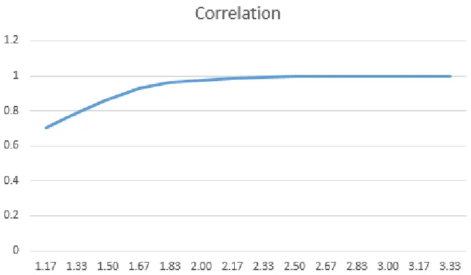
Figure 2: Experimentally breaking Lin-Matt candidate. Graph shows quality of recov-ered solution vs. planted solution, for various values ofm/nshown in the x-axis. Let vbe the eigen vector with largest eigen value of the optimum matrix returned by the SDP. Letxbe the planted solution. Quality of solution is defined as hv,xi
hv,vi12hx,xi12
6.3 Attacking polynomials of the form S+S+M Q
Now we consider attacking a more general form of systems where each polynomial qj(x1,x2,x3) is of the following form:
– qj takes as input three input vectorsx`= (x`,1, . . . , x`,n) for`∈[3].
– Then,qj =Sj,1(x1) +Sj,2(x2) +M Qj(x3)
Inputs x` for ` ∈ [3] are chosen as in the previous section. We observe that when we constrain the sum Σ`∈[2],j∈[n]x2`,n, then SDP successfully recovers the planted solution using about same number of samples (for the same size of input) as for the previous case. This code of the recovery functionrecoverspecialssm is given in Section A. Note that in the code, the sum val1+val2 is used to constrain this sum. This seems to generalise. If we consider a family where the polynomialsqare of the formS1+. . .+Sk+M Q1+. . .+M Qk, for values ofk
7
Cubic Assumption
In this section, we discuss the cubic assumption proposed by [2]. Let us first recall the cubic version of the ∆RGassumption considered by [2]. First, we define a notion of a polynomial samplerQ
Definition 6. (Polynomial Sampler Q) A polynomial samplerQis a probabilis-tic polynomial time algorithm that takes as inputn, B,∈Nalong with a constant
1> ε >0 and outputs:
– Polynomials(q1, ..., qbn1+εc).
– Each polynomial qj(e1, ..., en, y1, ..., yn, z1, ..., zn) = Σi1,i2,i3∈[n]ci1,i2,i3ei1yi2zi3. Here, each coefficient ci1,i2,i3 are
in-tegers bounded in absolute value by a polynomial in n and
e1, ..., en, y1, .., yn, z1, ..., zn are the variables of the polynomials.
Cubic ∆RGAssumption. There exists a polynomial sampler Qand a constant ε > 0, such that for every large enough λ ∈ N, and every polynomial bound
B = B(λ) there exist large enough polynomial nB = λc such that for every positive integern > nBthere exists an efficiently samplable bounded distribution χ that is bounded by some polynomial in λ, n such that for every collection of integers{δi}i∈[bn1+εc]with|δi|6B, the following holds for the two distributions
defined below:
Distribution dist1:
– Fix a prime modulusp=O(2λ).
– (Sample Polynomials.) Run Q(n, B, ε) = (q1, ..., qbn1+εc). – (Sample Secret.) Sample a secrets←Zλp
– Sampleai←Zλp fori∈[n].
– (Sample LWE Errors.) For every i ∈ [n], sample ei, yi, zi ← χ. χ is a bounded distribution with a bound poly(n) such that LW E assumption holds with error distributionχ, modulus pand dimensionλ.
– Output{ai,hai, si+ei modp}i∈[n],{qj, qj(e1, .., en, y1, ..., yn, z1, ..., zn)}j∈[bn1+εc] Distribution dist2
– Fix a prime modulusp=O(2λ).
– (Sample Polynomials.) Run Q(n, B, ε) = (q1, ..., qbn1+εc). – (Sample Secret.) Sample a secrets←Zλp
– Sampleai←Zλp fori∈[n]
– Output {ai,hai, si + ei modp}i∈[n],{qj, qj(e1, .., en, y1, ..., yn, z1, ..., zn) + δj}j∈[bn1+εc]
The assumption states that there exists a constant εadv > 0 such that for any adversaryAof size 2λεadv
, the following holds:
|P[A(dist1) = 1]−P[A(dist2) = 1]|<1−1/λ
Linearization Attack for n2 stretch. The assumption above is only required to hold for stretch n1+ε for any small constant ε. However, we observe that the assumption described above suffers from an attack if the stretch is O(λ·n2).
The attack is simple and is described below.
Theorem 5. The cubic ∆RG assumption does not hold with m = O(λ·n2)
polynomialsq1, . . . qm.
Proof. Here is the breaking algorithm. For notational convenience, we only con-sider homogenous degree-3 polynomials. In this case, we can setm=n2(λ+ 1).
However, the algorithm trivially generalizes to all degree-3 polynomials with m=n2(λ+ 3) + 2n+λ.
1. Consider a polynomial q`(e1, ..., en, y1, ..., yn, z1, ..., zn) =Σi,j,kci,j,k,`eiyjzk. 2. Rewrite q`(e1, ..., en, y1, ..., yn, z1, ..., zn) = Σi,j,kci,j,k,`(hai, si + ei − hai, si)yjzk. Now note that ai andbi =hai, si+ei is given. Setyjzk=wj,k andsindyjzk =wind,j,k forind∈[λ], j∈[n], k∈[n].
3. Note that since q`(e1, ..., en, y1, ..., yn, z1, ..., zn) = Σi,j,kci,j,k,`(bi −
hai, si)yjzk in Zp, the entire system of m = n1+ε samples can be written as a system of linear equations over Zp in (λ+ 1)n2 variables wind,j,k and wj,k. A simple gaussian elimination then recovers the solution.
On the existence of hard degree-3 polynomials. Feige [12] conjectured that its hard to distinguish a satisfiable random 3-SAT instance from a random 3-SAT instance with C·n clauses. Each disjunction x1∨x2∨x3 corresponds to the
polynomial 1−(1−x1)(1−x2)(1−x3). This intuition gives rise to a set of
candidate polynomials qi,j, which depends on three randomly chosen variables and maps{0,1}nto{0,1}. Eachqi,jhas at most 8 monomials. Intuitively speak-ing, to choose clauses, instead of chosing clauses at random – something that is known to lead to weak RANDOM 3SAT instances – we first choose a planted
to hard distributions, which suggests that the expanding polynomial systems corresponding to these clauses should be hard to solve in general.
To construct obfuscation, we need the stretch to be at least n1+ε for any constant ε > 0. All known algorithms take exponential time as long as n1.5−ε clauses are given out. This leads to a conjecture, which is also related to the work of [11]. As a result, we conjecture that the following candidate expanding family of degree-3 polynomials is hard to solve.
3SAT Based Candidate.. Let t = B2λ. Here, B(λ) is the magnitude of
the perturbations allowed. Sample each polynomial qi0 for i ∈ [η] as follows. q0i(x1, . . . ,xt,y1, . . . ,yt,z1, . . . ,zt) = Σj∈[t]q0i,j(xj,yj,zj). Here xj ∈ χd×n and yj,zj ∈χn for j ∈ [t]. In other words, qi0 is a sum of t polynomials q0i,j overt disjoint set of variables. Let χdenote a discrete gaussian random variable with mean 0 and standard deviationn. Now we describe how to sampleq0i,jforj∈[η].
1. Sample randomly inputsx∗,y∗,z∗∈ {0,1}n.
2. To sampleqi,j0 do the following. Sample three indices randomly and indepen-dentlyi1, i2, i3←[n]. Sample three signsb1,i,j, b2,i,j, b3,i,j ∈ {0,1}uniformly such thatb1,i,j⊕b2,i,j⊕b3,i,j⊕x∗[i1]⊕y∗[i2]⊕z∗[i3] = 1.
3. Setqi,j0 (xj,yj,zj) = 1−(b1,i,j·xj[i1] + (1−b1,i,j)·(1−xj[i1]))·(b2,i,j·yj[i2] +
(1−b2,i,j)·(1−yj[i2]))·(b3,i,j·zj[i3] + (1−b3,i,j)·(1−zj[i3]))
8
Acknowledgements
Boaz Barak was supported by NSF awards CCF 1565264 and CNS 1618026 and a Simons Investigator Fellowship. Samuel B. Hopkins was supported by a Miller Postdoctoral Fellowship and NSF award CCF 1408673. Pravesh Kothari was sup-ported in part by Ma fellowship from the Schmidt Foundation and Avi Wigder-son’s NSF award CCF-1412958. Amit Sahai and Aayush Jain were supported in part from a DARPA/ARL SAFEWARE award, NSF Frontier Award 1413955, and NSF grant 1619348, BSF grant 2012378, a Xerox Faculty Research Award, a Google Faculty Research Award, an equipment grant from Intel, and an Okawa Foundation Research Grant. Aayush Jain was also supported by Google PhD Fel-lowship 2018, in the area of Privacy and Security. This material is based upon work supported by the Defense Advanced Research Projects Agency through the ARL under Contract W911NF-15-C- 0205. The views expressed are those of the authors and do not reflect the official policy or position of the Department of Defense, the National Science Foundation, the U.S. Government or Google.
References
1. Agrawal, S.: New methods for indistinguishability obfuscation: Bootstrapping and instantiation. IACR Cryptology ePrint Archive 2018, 633 (2018), https: //eprint.iacr.org/2018/633 2,9,14
2. Ananth, P., Jain, A., Sahai, A.: Indistinguishability obfuscation without multilinear maps: io from lwe, bilinear maps, and weak pseudorandomness. IACR Cryptology ePrint Archive 2018, 615 (2018), https://eprint.iacr.org/2018/615 2, 3,9,
14,18
3. Ananth, P., Sahai, A.: Projective arithmetic functional encryption and indistin-guishability obfuscation from degree-5 multilinear maps. EUROCRYPT (2017) 1
4. Barak, B., Brakerski, Z., Komargodski, I., Kothari, P.: Limits on low-degree pseu-dorandom generators (or: Sum-of-squares meets program obfuscation). Electronic Colloquium on Computational Complexity (ECCC)24, 60 (2017) 2,7
5. Boneh, D., Silverberg, A.: Applications of multilinear forms to cryptography324 (11 2002) 2
6. Boneh, D., Wu, D.J., Zimmerman, J.: Immunizing multilinear maps against zeroiz-ing attacks. IACR Cryptology ePrint Archive2014, 930 (2014),http://eprint. iacr.org/2014/930 1
7. Brakerski, Z., Gentry, C., Halevi, S., Lepoint, T., Sahai, A., Tibouchi, M.: Crypt-analysis of the quadratic zero-testing of GGH. Cryptology ePrint Archive, Report 2015/845 (2015),http://eprint.iacr.org/ 1
8. Cheon, J.H., Han, K., Lee, C., Ryu, H., Stehl´e, D.: Cryptanalysis of the multilinear map over the integers. In: EUROCRYPT (2015) 1
9. Cheon, J.H., Lee, C., Ryu, H.: Cryptanalysis of the new clt multilinear maps. Cryptology ePrint Archive, Report 2015/934 (2015),http://eprint.iacr.org/ 1
10. Coron, J., Gentry, C., Halevi, S., Lepoint, T., Maji, H.K., Miles, E., Raykova, M., Sahai, A., Tibouchi, M.: Zeroizing without low-level zeroes: New MMAP attacks and their limitations. In: CRYPTO (2015) 1
11. Daniely, A., Linial, N., Shalev-Shwartz, S.: From average case complexity to im-proper learning complexity. In: STOC. pp. 441–448. ACM (2014) 20
12. Feige, U.: Relations between average case complexity and approximation complex-ity. In: STOC. pp. 534–543. ACM (2002) 19
13. Garg, S., Gentry, C., Halevi, S.: Candidate multilinear maps from ideal lattices. In: Advances in Cryptology - EUROCRYPT 2013, 32nd Annual International Confer-ence on the Theory and Applications of Cryptographic Techniques, Athens, Greece, May 26-30, 2013. Proceedings (2013) 1
14. Garg, S., Gentry, C., Halevi, S., Raykova, M., Sahai, A., Waters, B.: Candidate indistinguishability obfuscation and functional encryption for all circuits. In: 54th Annual IEEE Symposium on Foundations of Computer Science, FOCS 2013, 26-29 October, 2013, Berkeley, CA, USA. pp. 40–49 (2013) 1
15. Grigoriev, D.: Linear lower bound on degrees of positivstellensatz calculus proofs for the parity. Theor. Comput. Sci.259(1-2), 613–622 (2001) 3
https://doi.org/10.1109/TIT.2011.2104999, http://dx.doi.org/10.1109/TIT. 2011.2104999 7,11,12
17. Halevi, S.: Graded encoding, variations on a scheme. IACR Cryptology ePrint Archive2015, 866 (2015) 1
18. Hu, Y., Jia, H.: Cryptanalysis of GGH map. IACR Cryptology ePrint Archive 2015, 301 (2015) 1
19. Lin, H.: Indistinguishability obfuscation from constant-degree graded encoding schemes. In: Advances in Cryptology - EUROCRYPT 2016 - 35th Annual Interna-tional Conference on the Theory and Applications of Cryptographic Techniques, Vienna, Austria, May 8-12, 2016, Proceedings, Part I. pp. 28–57 (2016) 1
20. Lin, H.: Indistinguishability obfuscation from SXDH on 5-linear maps and locality-5 prgs. In: Advances in Cryptology - CRYPTO 2017 - 37th Annual International Cryptology Conference, Santa Barbara, CA, USA, August 20-24, 2017, Proceed-ings, Part I. pp. 599–629 (2017) 1
21. Lin, H., Matt, C.: Pseudo flawed-smudging generators and their application to in-distinguishability obfuscation. IACR Cryptology ePrint Archive2018, 646 (2018), https://eprint.iacr.org/2018/646 2,9,10,15
22. Lin, H., Tessaro, S.: Indistinguishability obfuscation from bilinear maps and block-wise local prgs. Cryptology ePrint Archive, Report 2017/250 (2017), http: //eprint.iacr.org/2017/250 1,2
23. Lin, H., Vaikuntanathan, V.: Indistinguishability obfuscation from ddh-like as-sumptions on constant-degree graded encodings. In: IEEE 57th Annual Sympo-sium on Foundations of Computer Science, FOCS 2016, 9-11 October 2016, Hyatt Regency, New Brunswick, New Jersey, USA. pp. 11–20 (2016) 1
24. Lombardi, A., Vaikuntanathan, V.: On the non-existence of blockwise 2-local prgs with applications to indistinguishability obfuscation. IACR Cryptology ePrint Archive2017, 301 (2017),http://eprint.iacr.org/2017/301 2
25. Miles, E., Sahai, A., Zhandry, M.: Annihilation attacks for multilinear maps: Crypt-analysis of indistinguishability obfuscation over GGH13. In: Advances in Cryptol-ogy - CRYPTO (2016) 1
26. Minaud, B., Fouque, P.A.: Cryptanalysis of the new multilinear map over the inte-gers. Cryptology ePrint Archive, Report 2015/941 (2015), http://eprint.iacr. org/ 1
27. Recht, B.: A simpler approach to matrix completion. Journal of Machine Learning Research12, 3413–3430 (2011) 11
28. Recht, B., Fazel, M., Parrilo, P.A.: Guaranteed minimum-rank solutions of lin-ear matrix equations via nucllin-ear norm minimization. SIAM Rev. 52(3), 471– 501 (2010). https://doi.org/10.1137/070697835, http://dx.doi.org/10.1137/ 070697835 7
29. Sahai, A., Waters, B.: How to use indistinguishability obfuscation: deniable en-cryption, and more. In: Symposium on Theory of Computing, STOC 2014, New York, NY, USA, May 31 - June 03, 2014. pp. 475–484 (2014) 1
A
Julia Code
function genmatrixDMQ(n, C) V = randn(n,n)
for i in 1:n for j in 1:n
V[i,j] = 0 end
end
for i in 1:n for j in i:n
V[i,j] = nr.randint(-C, high=C+1) end
end
(V’+V)/2 end
function genxMQ(n ,B) x = randn(n,1) for i in 1:n
x[i] = nr.randint(-B, high=B+1) end
x end
function genobsMQ(n,m,C,B)
L = [genmatrixDMQ(n,C) for i in 1:m] x = genxMQ(n,B)
obs = [x’*L[i]*x for i in 1:m] L,obs,x
end
function recoverMQ(L,obs)
n = size(L[1])[1] m = length(L)
# let’s maximize the trace @objective(model, Min, trace(X))
# this makes the constraints for i in 1:m
@constraint(model, trace(L[i]*X).==obs[i]) end
# this solves the problem solve(model)
getvalue(X)
end
function genmatrixsmq(n, n2, nprime, C) V = randn(n+nprime+2,n+nprime+2) Z = randn(n+nprime+2,n+nprime+2)
for i in 1:n+nprime+2 for j in 1:n+nprime+2
V[i,j] = 0 end
end
a=randperm(n)
#sparse monomials
for i in 1:n2
V[ a[2*i-1]+1,a[2*i]+1] = rand(-C:C) end
#MQ monomials
for i in n+3:n+nprime+2 for j in n+3:n+nprime+2
V[i,j] = rand(-C:C) end
#Linear terms in S
for j in 2:n+1
V[1,j]=rand(-C:C)
end
#Linear terms in MQ
for j in n+3:n+nprime+2 V[n+2,j]=rand(-C:C) end
Z=V’+V
Z
end
function genxdiscsmq(n,n2,nprime,B1,B2,Bprime) x = randn(n+nprime+2,1)
x[1]=1 x[n+2]=1
for i in n+3:n+nprime+2
x[i] = rand(-Bprime:Bprime) end
for i in 2:n+1
temp1=rand(-B1:B1) temp2=rand(-B2:B2) temp3=rand(0:1)
x[i] = (temp3*temp1+(1-temp3)*temp2 ) end
x end
L = [genmatrixsmq(n,n2,nprime,C) for i in 1:m] x = genxdiscsmq(n,n2, nprime,B1,B2,Bprime) obs = [x’*L[i]*x for i in 1:m]
L,obs,x end
function recoverspecialsmq(L,obs,n,n2,nprime,m,val1)
model = Model(solver = MosekSolver())
@variable(model, X[1:nprime+n+2,1:nprime+n+2], SDP)
# let’s maximize the trace @objective(model, Min, trace(X))
# this makes the constraints for i in 1:m
@constraint(model, trace(L[i]*X).==obs[i]) end
@constraint(model, X[1,1]==1) @constraint(model, X[n+2,n+2]==1)
@constraint(model, trace(X[1:n+1,1:n+1])=val1[1])
# this solves the problem solve(model)
getvalue(X)
end
function recoverspecialssm(L,obs,n,n2,nprime,m,val1, val2,val3) model = Model(solver = MosekSolver())
@variable(model, X[1:nprime+2*n+3,1:nprime+2*n+3], SDP)
# this makes the constraints for i in 1:m
@constraint(model, trace(L[i]*X).==obs[i]) end
@constraint(model, X[1,1]==1) @constraint(model, X[n+2,n+2]==1) @constraint(model, X[n*2+3,2*n+3]==1)
@constraint(model, trace(X[1:n+1,1:n+1]) + trace(X[n+2:2*n+2,n+2:2*n+2]) >= val1[1] + val2[1])
# this solves the problem solve(model)
getvalue(X)