Counting Keys in Parallel After a Side Channel
Attack
Daniel P. Martin, Jonathan F. O’Connell, Elisabeth Oswald, and Martijn Stam University of Bristol, Department of Computer Science,
Merchant Venturers Building, Woodland Road, BS8 1UB, Bristol, UK. {dan.martin, j.oconnell, elisabeth.oswald, martijn.stam}@bris.ac.uk
Abstract. Side channels provide additional information to skilled ad-versaries that reduce the effort to determine an unknown key. If sufficient side channel information is available, identification of the secret key can even become trivial. However, if not enough side information is available, some effort is still required to find the key in the key space (which now has reduced entropy). To understand the security implications of side channel attacks it is then crucial to evaluate this remaining effort in a meaningful manner. Quantifying this effort can be done by looking at two key questions: first, how ‘deep’ (at most) is the unknown key in the remaining key space, and second, how ‘expensive’ is it to enumerate keys up to a certain depth?
We provide results for these two challenges. Firstly, we show how to construct an extremely efficient algorithm that accurately computes the rank of a (known) key in the list of all keys, when ordered according to some side channel attack scores. Secondly, we show how our approach can be tweaked such that it can be also utilised to enumerate the most likely keys in a parallel fashion. We are hence the first to demonstrate that a smart and parallel key enumeration algorithm exists.
1
Introduction
Side channel attacks have proven to be a hugely popular research topic, as the proliferation of new venues such as CHES, COSADE and HOST shows. Much of the published research is about key recovery attacks utilising side channel information. Key recovery attacks essentially take a number of side channel ob-servations, colloquially referred to as ‘traces’, and apply a so-called distinguisher to traces that assigns scores to keys. An attack is considered (first-order) suc-cessful given a set of traces, if the actual secret key receives the highest score. Besides describing methods (i.e.the distinguishers) that recover the secret key from the available data, papers focus on the question of how many traces are required for successful first-order attacks.
The trade-off chosen in most work is, hence, to increase the number of traces to ensure that the secret key is recovered successfully with almost certainty. As observed by Veyrat-Charvillonet al.[17] in their seminal paper on optimal key enumeration, this might not be the trade-off that a well resourced adversary
would choose. Suppose that access to the side channel is scarce or difficult. In such a case the actual secret key might not have the highest score after utilising the leakage traces, but it might still have a higher score than many other keys. Now imagine that the adversary can utilise substantial computational resources. This implies that by searching through the key space (in order of decreasing scores; we call this smart key enumeration) the adversary would find the secret key much faster than by a na¨ıve brute-force search (i.e.one that treats all keys as equally likely). Consequently, the true security level of an implementation cannot be judged solely by its security against first-order side channel attacks. Instead it is important to understand how the number of traces impacts on the effort required for a smart key enumeration.
We now illustrate this motivation by linking it to evaluating the impact of the most influential type of side channel attack: Differential Power Analysis.
1.1 Evaluating Resistance against Differential Power Analysis
Differential Power Analysis (DPA) [11] consists of predicting a so-called target function, e.g. the output of the Substitution Boxes, and mapping the output of this function to ‘predicted side channel values’ using a power model. For this process it is not necessary to know or guess the whole secret key,SK. One only needs to make guesses about ‘enough bits’. The predicted values for a key chunk are then ‘compared’ to the real traces (point-wise) using a distinguisher. Assum-ing enough traces are available, the value that represents the correct key guess will lead to a ‘higher’ distinguishing value. In Kocheret al.’s original paper [11] this was illustrated for the DES cipher, but most contemporary research uses AES as running example.
With respect to AES: Kocher’s attack consists of using a t-test statistic as a distinguisher to compute scores for the values of each 8-bit chunk of the 128-bit key; see Fig. 1 for a visual example. Here we have m = 16 chunks, each containingn= 256 values, with associated distinguishing scores as derived via a t-test statistic. In the graphical illustration, the secret key values are marked out in grey.
If sufficient side information is available, the values of the chunks that corre-spond to the secret key will have by far the highest distinguishing scores, such as the majority of key chunks in our graphical illustration. In this case the secret key can be trivially found (it is the concatenation of the chunks that lead to the uniquely highest score). However, if less side information is available, the scores may not necessarily favour a single key. Nevertheless, an adversary is still able to utilise these scores to smartly enumerate and then test keys (by using a known plaintext-ciphertext pair).
Security evaluations Considering the perspective of a security evaluator, it is obviously important to characterise the remaining security of an implementation
0 1 2 3
n−2
n−1 k0 0.01 0.03 0.41 0.38 . . . 0.11 0.08
k1 0.01 0.13 0.11 0.27 . . . 0.01 0.02
k2 0.40 0.05 0.20 0.07 . . . 0.30 0.01
· · ·di,j· · · km−1
0.02 0.03 0.31 0.33 . . . 0.12 0.04
Fig. 1: Score vectors for m key chunks. Each chunk can take values from 0 to n−1, and scoresdi,jare on a scale that depends on the side channel distinguisher.
The values that correspond to the (hypothetical) secret key are highlighted in grey.
keys. Knowing this position allows the evaluator to assess the amount of effort required by an adversary performing a smart search (given some distinguishing vectors). Ideally, the evaluator is able to compute the ranks of arbitrarily deep keys.
Accuracy and efficiency are key requirements: Naturally, because the evaluator performs concrete statistical experiments, a single run of a single attack is not sufficient to gather sound evidence. In practice, any side channel experiment needs to be repeated multiple times by the evaluation lab, and many different attacks need to be carried out, utilising different amounts of side channel traces. Having the capability to determine the position of the key in a ranked list accu-rately (rather than just giving an estimation), and efficiently, is crucial to cor-rectly assess the effort of a real world adversary. Previous works’ algorithms [18, 8] were capable of estimating the key rank within some bound. We demonstrate that we are accurate when enough precision is used, and importantly, we put forward the first approach for parallel and smart key enumeration.
1.2 Problem statement and notation
We use a bold type face to denote multi-dimensional entities. Indices in su-perscript refer to column vectors (we use the variablej for this purpose), and indices in subscript refer to row vectors (we useifor this purpose). Two indices i, j refer to an element in rowi and column j. To maintain an elegant layout, we sometimes typeset column vectors ‘in line’, and then indicate transposition via a superscriptk= (. . .)T.
We partition a key guesskintomchunks, each able to take one ofnpossible values,i.e.k= k0, . . . ,km−1
, andkj= (d
0,j, d1,j, . . . , dn−1,j) T
. After exploit-ing some leakageLall chunkskj have some corresponding score vectors,i.e.we
know the score for each guess ki,j isdi,j after leakage. For convenience we use
the variable skj to refer to the indices (in each chunk) that correspond to the
correct key,i.e.SK= ksk1,1, ksk2,2, . . . , kskm−1,m−1
. The scoreD of the secret key is thenD=Pm−1
j=0 dskj,j. We will later map scores to (integer) weights and
the weight of the secret key will beW.
The rank of a key is defined as the position of the key in the ordering (of all keys), where keys with the exact same weight are ranked ‘ex aequo’. In principle, any order of these equally ranked keys is permissible, so one is free to make a choice about this order. Assuming the correct key is ranked first among all keys of the same weight requires us to count all keys with weight less than W. It implies that the rank we return is conservative in the following sense: key ranking is used to evaluate the security of side-channel attacks; our assumption on the ordering implies we give a side-channel adversary the benefit of the doubt (and so we deem it slightly more successful than it in reality can be). As an alternative, one could assume the correct key is ranked last among all keys of the same weight (since we use integer weights, this can be done by increasing the weight by one, counting all keys according to the ranked-first method, and subtracting one from the returned rank); ranking the candidate key both as first and last of its weight will lead to an interval of ranks containing all keys of that rank. Thus our choice (rank first) is effectively without loss of generality: run once it gives a conservative estimate, run twice it gives the exact interval of possible ranks for the candidate key.
Definition 1 (Key rank computation).Givenmvectors ofndistinguishing scores, and the score D of the secret key SK, count the number of keys with score strictly larger thanD.
Definition 2 (Smart key enumeration).Givenmvectors ofndistinguishing scores, list theB keys with the highest score.
1.3 Outline and our contributions
In a nutshell, we utilise an elegant mapping of the key rank computation problem to a knapsack problem, which can be simplified and expressed as (efficient) path counting. As a result, we can compute accurate key ranks, and importantly, this enables us to put forward the first algorithm that can perform smart key enumeration in a parallel manner.
Our contribution is structured in four main sections as follows:
A key rank algorithm. In Sect. 3 we map the multi-dimensional knapsack to a directed acyclic graph. We can therefore count solutions to the multi-dimensional knapsack problem by counting paths in the graph. The restric-tion of picking one item per chunk keeps the number of vertices in the di-rected acyclic graph small. As the graph is compact, and each node has at most two outgoing edges, the path counting problem can be solved efficiently inO m2·n·W·logn
.
Smart key enumeration. In Sect. 4, with the additional book-keeping of stor-ing the vertices we visit, we can enumerate theBmost likely keys with com-plexity O m2·n·W ·B·logn
. We then show several techniques to make this process as efficient as possible.
Practical evaluation and comparison with previous work. In Sect. 5 we discuss requirements around precision. The main factor that influences per-formance is the size of the key rank graph, which is determined by the pre-cision of the initial mapping and the weight of the target key. We compare our work with previous works in terms of precision and speed with regards to the key rank algorithm, and in terms of speed with regards to smart key enumeration.
1.4 Previous work
Key Rank An na´’ive approach is that by simply removing a number of the least likely key values from each key chunk, the size of the search space is then restricted asnis reduced. However there are inherit problems with the approach; firstly this may be removing valid high ranking keys, as it is possible that a key may be constructed from one very low ranked value in one key chunk, and very high in others. Secondly, it is still reliant on a simple brute force approach, and even with a reducednvalue this approach is thus too expensive to be practical. Finally, if the target key is deep, this approach won’t work at all as it is possible that the correct key values have been removed.
Veyrat-Charvillon et al. [18] were the first to demonstrate an algorithm to estimate the rank of the key without using full key enumeration. The search space can be represented as a multidimensional space, with each dimension cor-responding to a key chunk, sorted by decreasing likelihoods. The space can be divided into two, those keys ranked above the target and those ranked below. Using the property that the ‘frontier’ between these two spaces is convex, they are able to ‘trim’ each space down until the key rank has been estimated to within 10 bits of accuracy.
Bernstein et al. [2] propose two key ranking algorithms. The first is based on [18] and adds a post processing phase which has been shown to tighten the bounds from 10 bits to 5 bits. The second algorithm ranks keys using techniques similar to those used to count ally-smooth numbers less thanx. By having an accuracy parameter they are able to get their bounds arbitrarily tight (at the expense of run time).
Glowaczet al.[8] construct a novel rank estimation algorithm using convolu-tion of histograms. Using the property thatS1+S2:={x1+x2|x1∈ S1, x2∈ S2}
can be approximated by histogram convolution, by creating a histogram per key chunk and convoluting them all together, they are able to efficiently estimate the key rank to within 1 bit of precision.
Ducet al.[6] perform key rank using a method inspired by Glowaczet al.[8]. They repeatedly ‘merge’ the data in one column at a time (as the histograms were convoluted in one at a time). Each piece of information is downsampled to one of a series of discrete values (similar to putting into a histogram bin). The major difference is that instead of just downsampling the orginial data, they also downsample after each key chunk is merged in.
Key Enumeration Veyrat-Charvillon et al. [17] propose a deterministic al-gorithm to enumerate keys based on a divide-and-conquer approach. Using a tree-like recursion (starting with two subkeys, then four, all the way to sixteen) and keeping track of what they call the frontier set (similarities can be drawn to the frontier of Veyrat-Charvillonet al. [18]), they are able to efficiently enu-merate keys.
Yeet al.[19] present what they describe as a Key Space Finding algorithm. A Key Space Finding algorithm takes in the distinguishing score vector and returns two outputs: the minimum verification complexity to ensure a desired success probability, along with the optimal effort distributor which achieves this lower bound. Given this it is straightforward to run a (probabilistic) key enumeration algorithm. The distinguisher intuitively moves the boundary of which subkeys to enumerate until the desired probability is achieved.
Bogdanovet al. [3] create a score based key enumeration algorithm which can be seen as a variation of depth first search. Potential keys are generated via
score paths, each of which has a score associated with them, which in conjunction with a precomputed score table allows for efficient pruning of impossible paths. From here it is possible to efficiently enumerate possible values.
Reflecting on the approaches taken by previous work All of the previous work has treated key rank and key enumeration as two disjoint problems and hence approached them using different techniques. For instance, it is unclear how to extend the existing key rank algorithms to enumerate keys, and conversely, it is not apparent how to simplify the enumeration algorithms to compute key ranks efficiently (i.e. without just counting as you enumerate). We however believe that both of these problems are highly similar in nature and by maintaining some structure within the key rank it should be possible to enumerate without making the ranking inefficient. In the remainder of the paper we explain how to do just that: efficient key ranking with enough structure to make (fully parallel) enumeration possible.
2
Casting the key enumeration as a knapsack
of n items that have a profit pi and a weightwi. A binary variablexi is used
to select items from the set. The objective is then to select items such that the profit is maximised whilst the total weight of the items does not exceed a set maximumW:
maximize:
n−1
X
i=0
pi·xi
subject to:
n−1
X
i=0
wi·xi≤W
xi∈ {0,1},∀i
The counting knapsack (#knapsack) problem is then understood to be the associated counting problem: given a knapsack definition, count how many so-lutions there are to the knapsack problem.
Intuitively, we should be able to frame the key rank computation problem as a knapsack variant. In contrast to a basic knapsack, however, we have classes of items (these are the distinguishing vectors kj), profits can be dropped since we
are counting the number of solutions, and we must take exactly one item from each class. The weightwi,j for each item can be derived1from the distinguishing
scorewi,j=M apT oW eight(di,j) in such a way that higher distinguishing scores
lead to lower weights2. We define the maximum weight W as the sum of the
weights associated with the secret key chunks, i.e. W = Pm−1
j=0 wskj,j. Recall
that we assume if several keys have weight W the secret key (which must be among those) is listed first. This enforces W as a strict upper bound in the knapsack definition.
The multiple-choice knapsack problem that identifies keys with weight lower thanW is then defined as follows:
m−1
X
j=0
n−1
X
i=0
wi,j·xi,j< W
n−1
X
i=0
xi,j= 1,∀j
xi,j∈ {0,1},∀i, j
The first constraint ensures that all keys (i.e. selections of items) have a weight lower than the secret key. The second constraint ensures that only one item per distinguishing vector is selected. The counting version of this multiple-choice knapsack equals to computing the key rank.
1
For the sake of readability, we do not discuss the implications of needing to map distinguishing scores (which are floating point values) to weights at this point, but refer the reader to Sect. 5.1 for a discussion.
2
This ensures compatibility with knapsack notation.
Counting solutions to knapsack problems in general is known to be a compu-tationally hard problem, and known classical solutions [7] rely on combinations of dynamic programming and rejection sampling to construct an FPRAS. Gopalan
et al. [9] more recently utilise branching programs for efficient counting, and we took inspiration from this paper to approach the solution to our counting problem.
To illustrate our solution, we have to slightly modify the knapsack repre-sentation. It will be convenient to express the multiple-choice knapsack as a multi-dimensional knapsack variation as follows. Each key chunk corresponds to ‘one dimension’. Each item ki,j has an associated weight vector wi,j of length
m+ 1 of the form (wi,j,0, . . . ,1,0, . . . ,0), where the 1 is in position j. The
global weight is also expressed as a vectorW = (W,2, . . . ,2) of length m+ 1. The key rank problem is then to count the number of solutions (that satisfy all constraints simultaneously) to
m−1
X
j=0
n−1
X
i=0
wi,j·xi,j<W
xi,j∈ {0,1},∀i, j
The constraintW ensures that all keys that are counted have a strictly lower weight than the secret key. If the weight vector has a 1 in position j, it means that this is a value for the jth key chunk. Since the weight limit is 2 in the
constraint vectorW, it means that only a single value for any key chunk can be chosen. We now illustrate this by a simple example.
Example 1. Our illustrative example, which will run throughout the paper, con-sists of two distinguishing vectors with three elements each:k0= (0,1,3)T
, and
k1 = (0,2,3)T
. We assume that the secret key, SK, is (2,1). First we derive the global weight constraint vector. In this case it has length m+ 1 = 3 and contains the maximum weight W =w0,2+w1,1 = 3 + 2 = 5, which results in
W = (5,2,2). The weight vectors of theki,j are:
w0,0= (0,1,0),w0,1= (1,1,0),w0,2= (3,1,0)
w1,0= (0,0,1),w1,1= (2,0,1),w1,2= (3,0,1)
Given thatW = 5, all except two of the combinations are below this thresh-old. Hence the solutions to the knapsack are:
(k0,0, k0,1),(k0,0, k1,1),(k0,0, k2,1),
(k1,0, k0,1),(k1,0, k1,1),(k1,0, k2,1),
Notice that the knapsack solution will never contain the secret key itself, as it returns all keys with weightstrictly less than the weight of the secret key. For the ranking problem this would give us that our secret key has rank 8.
For standard knapsack problems it is well known [5] that solutions can be found via finding longest paths on a directed acyclic graph. In the following section we will show that such a graph exists also for our knapsack, and impor-tantly, that the resulting graph allows for a particularly efficient path counting solution, which gives us a solution to the Key Rank problem.
3
An accurate key rank algorithm
In this section we first define the graph and illustrate how it relates to the multi-dimensional knapsack via intuition and a working example. We then explain our fast path counting algorithm for a compact representation of the graph.
3.1 Key rank graph
Recall that our multi-dimensional knapsack has m·n elements, and for each element we have a weight vector. Also, a correct solution to the multi-dimensional knapsack must have a weight that is strictly smaller thanW. Since we need to be able to represent all permissible solutions we need W extra vertices (per element). This means that we ‘encode’ all solutions to the knapsack in a graph with m·n·W vertices (plus an extra two for accept and reject nodes). The vertices corresponding to itemki,jare labelledVi,jw, where the variablewdenotes
the ‘current weight’. The key rank graph contains a start nodeS, an accept node Aand a reject nodeR. The edges are constructed as follows:
– Vi,jw, Viw+1,jwhich corresponds to the item not being chosen in this set – Vw
i,j, V
w+wi,j
0,j+1
if the item is chosen for this set andw+wi,j< W
– Vn−w1,j, Rif no elements are chosen from the set – Vw
i,m−1, A
if the item is chosen for the last set andw+wi,m−1< W
– Vw
i,j, R
if the item is chosen for this set andw+wi,j≥W
– S=V0
0,0to set up the start node
When visualising the key rank graph it will be convenient to think of the indicesi, j as though they are ‘flattened’ (i.e.they are topologically sorted and occur in a linear order). In this representation the graph isn·mdeep,W wide, where the width of the key rank graph essentially tracks the current weight (of the partial keys). Each vertex has exactly two edges coming out of it (with the exception ofAandR): either the vertex was ‘included’ (this corresponds to the choice of selecting the corresponding value of the key chunk to become part of the key) or not. If the answer is yes then the edge must point to the first item in the next key chunk, as we can only choose one item per key chunk, and the weight must be incremented by the weight of this key item. If the item/vertex is
not chosen then the edge must go to the next item in the chunk (or reject if this was the last item) and the weight must not be incremented as the item was not selected. For any partial key, if a new key chunk is added and the new weight exceeds W then this is not a valid key and thus the path will go to the reject nodeR.
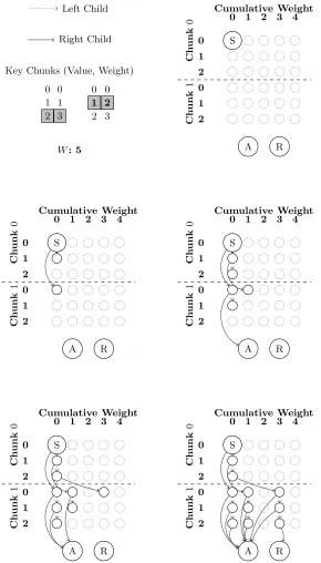
Graph Example To illustrate the working principle we provide in Fig. 2 the process of constructing the graph for the example provided above.
Initially the graph is constructed (top right) and the start node is initialised based on the ruleS =V0
0,0. The width of the graph is set to be 5 (0-4) as this
matches our maximum weight (W = 5). The depth of the graph becomes 6 as each chunk contains 3 items.
Next (middle left) the first two children from the start node are created. The edge that denotes the chunk is, in fact, selected (the right child) is built following the rule V0
0,0, V 0+0 0,1
, which creates the edge from the start node, to an element in the next chunk. The edge that denotes the chunk is not selected (the left child) is built following the rule V0
0,0, V10,0
, which creates the edge from the start node to the next item within the same chunk.
Moving onto the following step (middle right), children continue to be created through the same set of rules. However, note that at the point a link is created to the accept node based on the rule V0
0,1, A
, this demonstrates that the selection of key chunk 0 followed by 0 is a valid solution to the problem.
In the following steps links continue to be created based on the rules until all paths in the graph are created. Please note that throughout the construction of the graph, the last item in each chunk will have a left child that points to reject (as obviously there are no further chunks to select) but these have been omitted from the example diagram for the sake of clarity.
All the greyed out nodes also have their children calculated. However, as they do not alter the path count, we have excluded them from the example figures to aid clarity.
Each path fromS to Aif, corresponds to a key with lower weight than our secret key. Thus, counting these paths will yield the rank of the secret key. While in general path counting is hard [16], we explain how our graph structure, having at most two outgoing edges per node, lends itself to efficient counting.
3.2 Counting valid paths
Clearly our key rank graph is a directed acyclic graph. We have already men-tioned that it is convenient to ‘flatten’ the graph (as it has been presented in the example). This ‘flat’ graph is also more suited for an efficient counting al-gorithm. Hence, from this point onwards we will now assume that the graph is topologically sorted3. The start node will be labelled 1 and the final node
3
excep-Key Chunks (Value, Weight) 0 0 1 1 2 3 0 0 1 2 2 3 Left Child Right Child
W: 5 A R
S
0 1 2 3 4
Cumulative Weight 0 1 2 0 1 2 Ch unk 0 Ch unk 1 A R S
0 1 2 3 4
Cumulative Weight 0 1 2 0 1 2 Ch unk 0 Ch unk 1 A R S
0 1 2 3 4
Cumulative Weight 0 1 2 0 1 2 Ch unk 0 Ch unk 1 A R S
0 1 2 3 4
Cumulative Weight 0 1 2 0 1 2 Ch unk 0 Ch unk 1 A R S
0 1 2 3 4
Cumulative Weight 0 1 2 0 1 2 Ch unk 0 Ch unk 1
Fig. 2: An example showing the construction of the graph for the small example
will be labelledA. There aren·m·W + 2 vertices in the graph, we have that A=n·m·W+ 2 and R=A−1.
We also assume two constant time functionsLC(·),RC(·) which return the index of the left child and right child, respectively. The algorithmic descriptions of these functions can be found in App. B for our particular graph. We therefore have the following recurrence relation, where P C is a vector and P C[i] stores the number of accepting paths fromitoA:
P C[c] =
1, ifc=A.
0, ifc=A−1.
P C[LC(c)] +P C[RC(c)], otherwise.
The total number of paths between 1 (our start node) and A (our accept node) is then simplyP C[1]. This recurrence relation forms the algorithm given in Fig. 1, which assumes thatLC, RC are globally accessible functions.
Algorithm 1 The key rank algorithm
P C[A]←1
forc=A−1toi= 1 do
P C[c]←P C[LC(c)] +P C[RC(c)] end for
return P C[1]
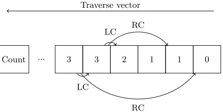
For an example of this, see Fig. 3. This figure shows that the vector is tra-versed from the end back to the start, and cells are filled by summing the values in their left and right children cells. For clarity in the figure, we only show example links betwen two cells, whereas in practise they are present on all.
Correctness The base case ofP C[A] = 1 is self explanatory; there is exactly one path from A toA, the path involving no edges. From an arbitrary nodec, it is possible to traverse the edge to the left child (and thus take however many paths start there) or traverse the edge to the right child (and do the same) and we conclude that P C[c] = P C[LC(c)] +P C[RC(c)]. We can iterate over all nodes starting at the final node A and working backwards until we reach the start node, and since our graph is topologically sorted when we are operating on a node, the values for the nodes’ children will already have been calculated as they come later in the topological sorting.
We note at this point that this counting algorithm isexact. However, as we pointed out before, we need to convert floating point distinguishing scores to integer weights, and this conversion may incur a loss of precision and hence could cause a loss of accuracy. We discuss this in Sect. 5.
Count ... 3 3 2 1 1 0 RC
LC
RC LC
Traverse vector
Fig. 3: Example demonstrating how the path count is calculated. Two nodes children links have been included to demonstrate the process.
Time complexity The time complexity of the key rank algorithm depends on the number of vertices in the key rank graph and their size. Our graph contains A=m·n·W vertices. The integers stored in the vertices could be up toO(2A) (and thus be of size O(A)) because in the worst case each value can be double the previous value (if P C[LC(i)] =P C[LC(i)]). Hence, given that we have A vertices and perform an integer addition with anA-bit variable for each vertex, we have worst-case time complexity ofO(A2) =O(m2·n2·W2).
However, whilst we touch each vertex once, we know that there are at most O(nm) keys. Consequently, we need no more than O(mlogn) bits to store the
path count (in contrast to the O(A) = O(m·n·W) bits for the worst case). Hence the time complexity for computing the key rank via the key rank graph isO(m2·n·W ·logn).
It is worth noting that the key depth does not factor into the time complexity and the following example will help to clarify this. Consider the target key which has weight 1 in every column (which givesW = 16 and a grid with 65536 nodes). If all other key chunks have weight 0 then the target key will have rank 2128since
all other keys have a lower weight. However, if all other key chunks have weight 2, then our target key will have rank 0 because all other keys have a higher weight. None of the other values affect the size of the graph and thus it is clear that the runtime is not changed by the key depth.
In fact for AES-128 the values of m, n are also fixed and thus we get that the algorithm runs inO(W), that is to say it is linear in the weight of the secret key. See Sec. 5.1 for experiments supporting this.
4
Parallelisable key enumeration algorithm
We are able to further modify our algorithm such that with minor (standard book-keeping) adjustments, we are able to list all valid paths, as opposed to just counting them, with reasonable efficiency. The algorithm is given in Alg. 2 and requires an additional (constant time) function callvalue which, given an index c, returns the value of a vertex. We write (a,{xc}c) to mean{(a, xc)}c. That is
Algorithm 2 The key enumeration algorithm
KL[A]← ∅ forc=Ato1do
KL[c]←(value(c), KL[RC(c)])∪KL[LC(c)] end for
return KL[1]
to say if we concatenate an item a with a set, we are really concatenating the itemawith every item in the set to form a new set.
It is now easy to use this for key enumeration. Assume we have the resources to enumerate/test up to B keys. Then, we choose some weights (which corre-spond to key guesses) and use the key rank algorithm to determine their ranks and compare them toB. This allows us to quickly select the appropriateW for the given B. Then, Alg. 2 proceeds as follows: for any valid path (in the key rank graph), every time a right child is taken (this can be determined by the node indices) the corresponding value for the respective key chunk is chosen. A left child means that we are not taking a particular value for key chunk. In this manner the keys are effectively reconstructed from the key rank graph.
If one wanted to enumerate the keys in a smart order, this would simply be a case of altering the construction of the tree which stores the valid key chunks for enumeration. Currently the valid key chunks are stored in numerical order within the tree, however if this was changed such that they were stored in order of scores, the keys would be rebuilt in a near optimal order.
In the rest of this section we discuss run time and memory requirements. Whilst the run time is bounded by the number of keys that we want to enu-merate, we show there there are different strategies to improve the memory performance. Finally, we show that with a further simple observation, we can parallelise the key enumeration algorithm.
4.1 Time complexity
We begin with a worst case analysis considering a general graph. In this case, the enumeration algorithm would be exponential in the length of the number of vertices, because to generate all paths (each vertex has two children) the algorithm clearly must takeO(2A) time.
However, in our key rank graph, each path corresponds to a valid key with weight lower thanW. Considering this, the run time of this algorithm is relative to the rank (which is determined by W) and not to the total number of keys; hence this algorithm can be used to enumerate keys for a given workload in time O(m2·n·W·B·logn). This is because allO(n·m·W) nodes are touched once,
4.2 Memory efficiency
How we topologically sort the key rank graph has a major impact on the memory efficiency of the key enumeration. While there are a variety of explicit topological sorting algorithms in the literature [10, 15], we are able to avoid explicit sorting because we know our graph structure in advance. Hence, we show that our graph can be sorted implicitly by how the nodes are numbered within the calculation of the left and right child functions. The remaining question is what method of sorting is the most desirable.
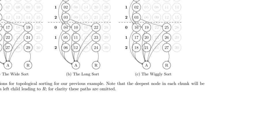
In Fig. 4 we give the three options of topologically sorting the example graph previously considered in Fig. 2. Appendix B gives the pseudo-code for the left and right children functions for each of the three topological sorts given below. We discuss the pros and cons of each of the sorting methods. We also discuss how to improve memory efficiency further by appropriately storing the generated keys.
Wide Sort In this sorting the graph is numbered one chunk at a time, one item at a time, along the weight in increasing order (see Fig. 4a). Formally given a chunk, item and weight (x, y, z) the index isi=x·W ·n+y·W+z. This is a valid topological sorting of the graph, since a nodes’ children will be either one item lower in the same chunk (for the left child) or the the first item in the next chunk (right child) both of which have a higher number.
This is the topological sort we described for key rank. Note that, since key rank is extremely fast we describe the most intuitive sort since it did not have an impact on performance, while with enumeration this is no longer the case and must now be taken into consideration.
The advantage of this sorting is that it is due to the fact an element will only need to look at the item below and the item at the top of the next chunk; these are the only things needing to be stored in memory. This makes it very memory efficient requiringO(W) memory.
The disadvantage of this method is that it is highly serial and it does not seem possible to (easily) parallelise.
Long Sort In this sorting the graph is numbered one weight at a time, one chunk at a time, along the item in increasing order (see Fig. 4b). Formally given a chunk, item and weight (x, y, z) the index is i=z·n·m+x·n+y. This is a valid topological sorting of the graph, since the left child will have the same weight but higher item number and thus will have a higher number, while the right child will have either the same weight or a higher weight for the next chunk and thus will have a higher number.
The advantage with this sorting is that (with careful synchronisation) it can be made parallel along the weights. Since the left child is always in the same weight this requires no synchronisation as it will be computed by the same process. The only time that synchronisation is needed is when the right child is calculated because this could have larger weight and thus would be calculated by
a different process. Therefore it is required that for a process to calculate a right child all processes running with higher weights have finished with the previous chunk before this process can begin.
The disadvantage with this method is that no clever memory tricks can be performed and thus the whole thing needs to be stored in memory at once, requiringO(n·m·W) space.
Wiggly Sort In this sorting the graph is numbered one chunk at a time, one weight at a time, along the item in increasing order (see Fig. 4c). Formally given a chunk, item and weight (x, y, z) the index isi=x·W·n+z·n+y. This is a valid topological sorting because the left child will be one further down within the same weight and within a chunk we are calculating items down the same weight. The right child will be in the next chunk and we are calculating one chunk at a time.
This sorting combines the advantage of the previous two with none of the disadvantages. Within each chunk the individual weights can be run in parallel because it either relies on information in the same weight or information from item 0 in the previous chunk (which has already been calculated). Hence as long as all threads syncronise at item 0 in each chunk the rest can be calculated in parallel. Since we only require information in our current chunk and the item 0 from the previous chunk, memory can be reused giving a memory requirement ofO(n·W) which, while not as good as the first (serial) method, is better than the second (parallel) method.
Key Storage The topological sorting of the graph is clearly a crucial factor for memory efficiency. The other factor is how keys are represented/stored within our graph.
In the algorithm as described all (partial) keys are stored at each point in the algorithm. This will become very inefficient. Consider, for example, the case where you want to enumerate all keys. There are 2120 keys which have the first
key chunk set to zero (hence this chunk would be duplicated 2120times). Clearly,
A R 01 06 11 16 21 26 02 07 12 17 22 27 03 08 13 18 23 28 04 09 14 19 24 29 05 10 15 20 25 30
0 1 2 3 4
Cumulative Weight 0 1 2 0 1 2 Ch unk 0 Ch unk 1
(a) The Wide Sort
A R 01 02 03 04 05 06 07 08 09 10 11 12 13 14 15 16 17 18 19 20 21 22 23 24 25 26 27 28 29 30
0 1 2 3 4
Cumulative Weight 0 1 2 0 1 2
(b) The Long Sort
A R 01 02 03 16 17 18 04 05 06 19 20 21 07 08 09 22 23 24 10 11 12 25 26 27 13 14 15 28 29 30
0 1 2 3 4
Cumulative Weight 0 1 2 0 1 2
(c) The Wiggly Sort
Fig. 4: Different options for topological sorting for our previous example. Note that the deepest node in each chunk will be guaranteed to have a left child leading toR; for clarity these paths are omitted.
A B
A B A B
A B A B A B A B
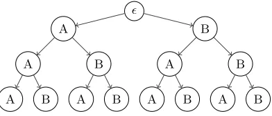
Fig. 5: The key tree for all possible three character keys containing ‘A’ or ‘B’
4.3 Parallelisation
We can achieve parallelisation with a simple observation: by adjusting the graph such that instead of vertices with a weight lower than W going to the accept state, we only allow vertices with weight in the range between the two weights W1 and W2 to reach the accept state. The width of the graph is defined by
W2; W1 has no impact on the graph size. This results in an algorithm that
enumerates ‘batches’ of likely keys. Hence, one can run multiple instances of the key enumeration algorithm in parallel, where each instance enumerates a unique batch of keys.
All ranges of keys can be computed in parallel and require no communication between threads except for the initial passing of the distinguishing scores and a notification when the key has been found. It is hence trivial to utilise multiple machines (or cores).
Setting W In an enumeration setting, the correct key, and thereforeW is un-known. We create a series of ‘steps’ inW (to bound usingW1,W2as introduced
previously), which are enumerated in order until the correct key is found. Iterating across these W increments, we select the weights by first taking the most probable across all distinguishing vectors,i.e.the weight at the top of each column. If the correct key is not located, the weight limit is increased by an amount equal to moving down by one key chunk in a column. The generation of eachW step is done according to the following:
More complex methods of bounding the weights could be used, such as binary searches or similar, but this would increase the cost of calculating the capacities before the enumeration begins, with little tangible benefit.
Algorithm 3 GeneratingW increments for enumeration whenW is unknown fork= 0 tomdo
c←00,...,m fori=ktomdo
forj= 0tondo
ci+ 1
CalculateW of key chunks at depthsc
end for end for end for
Further speed optimisations. Currently the algorithm operates on every node of the graph. However, some of the nodes are not even reachable from the start node (for example the greyed out nodes in Fig. 2). Hence any computation done on these nodes is wasted because it will never be combined into a solution. By precalculating the number of valid paths fromSto all other nodes in the graph (a reasonably cheap operation compared to a large key enumeration – this is done using the key rank algorithm), we can skip over a node if the number of paths from the start node to here is 0 because any work here will not be combined with the final solution.
5
Practical evaluation and comparison with previous
work
Our key enumeration and key rank algorithms are both based on a graph rep-resentation of a multi-dimensional knapsack. To define this multi-dimensional knapsack it is necessary to map distinguishing scores, which typically are float-ing point values, to integer weights. This requirement has implications for the performance of our algorithms, as the time complexities for both algorithms strongly depend on the parametersm(the number of key chunks),n(the num-ber of items per chunk), and W (the maximum weight). In particular, for any fixed key size (and number of chunks) the size of the graph (i.e.the width) grows withW, andW grows with the precision that we allow for in the conversion from floating point values to integers.
We hence focus our practical evaluation on the impact of the precision4, on accuracy5 and on performance. First, we discuss the precision requirements for practical DPA outcomes. Second, we explore the practical impact on the performance of key rank when we increase the precision. Third, assuming we allow for sufficient precision, we ask what are the best performance results that we can achieve on single but also many core platforms for the key enumeration.
4
Precision is the ability to reproduce a measurement result, i.e.if several measure-ments of a variable give very close values then the measurement is precise.
5
Accuracy is the closeness of a measurement to a true value,i.e.this relates to the ‘trueness’ of a measurement.
It is clear that to answer these questions we need to be able to generate many practically relevant distinguishing vectors in a manner that is comparable to previous work. We hence decided to adopt the simulator used by Veyrat-Charvillonet al.[17], which we explain in App. A.1 in more detail. In a nutshell, Veyrat-Charvillon et al. create distinguishing vectors based on attacking the AES SubBytes output, assuming noisy Hamming weight leaks, and using the Hamming weight as power model. Their DPA simulator allows to manipulate the level of noise, and the number of measurements. They output ‘additive’ scores (by taking the logarithm of the raw matching scores), which we pass directly to ourM apT oW eightfunction (see A.2).
5.1 Evaluating and comparing precision
In practical DPA attacks the combination of measured power traces, model val-ues, number of traces and distinguisher will influence theeffectiveprecision of the distinguisher scores6 We discuss the mentioned factors briefly. Then we
experi-mentally determine the necessary level of precision for our key rank algorithm, and compare this to the number of bins for the method by Glowaczet al.[8].
Precision in factors influencing DPA outcomes.
Leakage traces: Modern scopes offer between 8 and 12 bits of vertical reso-lution. Dedicated AC/DC converters may achieve up to 16 bits of vertical resolution; however, they can only achieve this at low sampling frequencies (hence modern scopes opt for lower resolution but allowing higher sampling frequencies). This vertical resolution, however, is for all the points in a trace. Consequently, the resolution in a single point will be much lower7. The loss
of precision can be compensated for by averaging over several measurements: this is effectively utilised by DPA attacks because typically many more power traces are measured than there are power models. In a well-known paper, Azizet al. [1] derive that to increase the precision of some data byb bits, the oversampling rate needs to be 4b.
Power model: Many practical DPA attacks use the Hamming weight or Ham-ming distance to map the target values to predicted power consumption val-ues. In the case of profiled attacks, the literature reports so-called stochastic models [14] (which model power consumption as a linear function in the bits of the target) mainly for 8-bit targets, and template attacks [4]. Template attacks can be run in different ways [12] utilising betweent, 2tor even 2t×2t
distinct power models for at-bit target. Consequently, practical template at-tacks typically remain restricted to 8-bit targets, or do not utilise the full
6 Veyrat’s simulator stores values in variables with double precision (i.e. one has 53
bits of precision). But effectively, only a few of them are necessary to contain the effective precision.
7
Bits
5 6 7 8 9 10 11 12 13 14 15 16
Key Rank Difference (log
2
)
0 5 10 15 20 25 30
Bits
5 6 7 8 9 10 11 12 13 14 15 16
Key Rank Difference (log
2
)
0 5 10 15 20 25 30
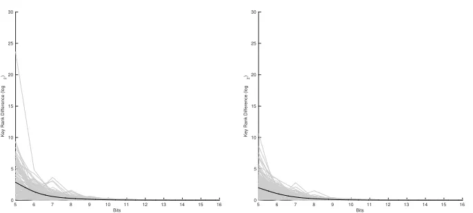
Fig. 6: Impact of the distinguisher (left: correlation, right: Gaussian templates without log2) on the precision requirements when considering up to 16 bits of precision.
set of templates. This brief overview shows that the precision of the power model is actually quite low.
Distinguisher: We speculate that distinguishers that require ‘simple opera-tions’, such as additions, subtractions, etc. of floating point values require less precision than distinguishers that e.g. include computing logarithms. Any confirmation for this hypothesis can only come from practical experi-ments, given the lack of work on this question.
Experimentally measuring precision for key rank and Glowacz et al.
We ran precision tests using Veyrat-Charvillon’s simulator (see A.1, usingN = 30 and variance two) to determine the appropriate level of precision for further experiments. We plot the difference in ranking outcomes for increasing precision in Fig. 7 (left). In this figure, and in all figures that will follow, we plot outcomes of individual experiments in gray, and average outcomes in black. The x-axis show the precision inwi, j. They-axis refers to the change in ranking outcomes
when increasing the precision by 0.1 bits from the previous step. From 11 bits onwards the outcomes do not change anymore. Because our ranking method is exact with enough precision, we can infer that with 11 bits of precision inwi,j
we produceexact ranks. Already from 4 bits of precision (on average, as plotted in black) we are within five bits of accuracy from the real result. From about 8 bits onwards, increasing the precision changes the ranking outcomes by just under a bit for our algorithm.
We implemented the convolution based method by Glowaczet al.[8]. Their method is essentially based on building m histograms (one from each of the distinguishing vectors) and counting the keys by counting items in the ‘amal-gamated’ histogram efficiently via convolution. Figure 7 (right) shows that they
Bits
5 6 7 8 9 10 11 12 13 14 15 16
Key Rank Difference (log
2
)
0 5 10 15 20 25 30
Number of Bins ×105
0 0.5 1 1.5 2 2.5 3 3.5 4 4.5 5
Key Rank (log
2
)
0 0.1 0.2 0.3 0.4 0.5 0.6 0.7 0.8 0.9 1
Fig. 7: Bits of precision for Key Rank (left) and number of bins for Glowacz et al.(right).
achieve very high average precision (plotted in black) from about 50,000 bins on-ward. We can therefore conclude that using 50,000 bins roughly corresponds to 11 bits of precision inwi,j. Glowaczet al.[8] actually recommend to use 500,000
bins in their paper.
Recall that we hypothesised that different distinguishers would lead to differ-ent precision requiremdiffer-ents. To test this hypothesis we implemdiffer-ented two further distinguishers for the simulator: one distinguisher was based on correlation and one was based on Veyrat-Charvillon’s method but without applying the loga-rithm. Figure 6 shows the results for them, this time we allowed up the 16 bit precision. The plots show that indeed, different distinguishers require different levels of precision, and that correlation has the least requirements.
To provide further evidence for the exactness of our ranking algorithm (pro-vided enough precision), we considered the difference between the key rank out-put by our algorithm, and the key rank outout-put by Glowaczet al.. In this experi-ment, we used 16 bits for our algorithm and 500,000 bins for Glowaczet al.Fig 8 shows the identical trend as Fig. 1 (right panel) of Glowaczet al.. Hence the dif-ference between our ranking outcomes and their ranking outcomes are identical to the rank estimation tightness that they measure, reinforcing the exactness of our ranking outcomes.
5.2 Evaluating and comparing run times for key rank
Key Depth (log2)
0 5 10 15 20 25 30 35 40
Difference (log
2
)
0 0.1 0.2 0.3 0.4 0.5 0.6 0.7 0.8 0.9 1
Fig. 8: Observed difference in calculated key rank between our algorithm and Glowaczet al.
We hence experimented with the relationship between run time and size ofW and also precision. We did this by fixing all parameters for Veyrat-Charvillon’s simulator and only varying the precision allowed in the functionM apT oW eight. As in the previous graph, we upper bounded the precision inW at 16 bits.
Figure 9 shows how the run time increases for bigger W (left) and more precision inW (right). The run times for sufficient precision (i.e.8 bits forW) are well below half a second. Even with 11 bits of precision (i.e.accurate ranking outcomes) our average run time is around 4 seconds. The plot shows that this average (black) is tracked well by the individual experiments (gray).
5.3 Evaluating and comparing run times for key enumeration
The run time of the key enumeration algorithm (as referred to by KEA in the graphs that will follow) is dominated by the depth to the key. Veyrat-Charvillon
et al.[17] presented the current state of the art for smart key enumeration, and they kindly gave us access to the latest version of their implementation. We were hence able to run their code alongside ours. Therefore for all graphs that we provide in the following, the timings were obtained on identical platforms. Note that for all experiements, as the toolbox provided a known secret key on which the simulated attack was based, we knew at which point the enumeration had found the correct key without needing to performm an AES operation on a known plaintext/ciphertext pair (this is common within the literature).
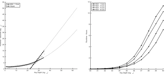
Single core vs multi core comparisons. Figure 10 gives a comparison of run times of Veyrat-Charvillonet al.’s algorithm and our algorithm on a single core (left). We sampled multiple distinguishing scores for each key depth and ran our respective key rank algorithms. The graphs show that from key depths just under 30 bits onwards we clearly outperform Veyrat-Charvillonet al.’s algorithm, even on a single core. On the right, we provide some performance graphs when running
Graph Width ×105
0 0.5 1 1.5 2 2.5 3 3.5 4 4.5 5
Runtime - Seconds
0 20 40 60 80 100 120
Bits
4 6 8 10 12 14 16
Runtime - Seconds
0 20 40 60 80 100 120
Fig. 9: Impact of the size ofW (left) and precision inwi,j(right) on the run time
of Key Rank
our key enumeration algorithm on multiple cores. The graph shows that eight cores can enumerate 240keys in the same time as one core enumerates 237, which
is a vast difference. Also another result of note is a single core run enumerates 238
keys in 13.9 hours and four cores performs the same enumeration in 6.4 hours.
A
Implementation Details
A.1 Veyrat-Charvillon’s distinguishing score simulation
Veyrat-Charvillon’s toolbox simulates a DPA attack using Hamming weight both as the power model and as the leakage function. It targets the SubBytes output (via exclusive-or between a plaintext byte and corresponding key byte, which is then used as input for SubBytes). For the leakage traces (each leakage trace consists of a single leakage value), random noise (i.e.sampled from a Gaussian distribution with zero mean and adjustable variance) is added to the Hamming weight of the SubBytes output (as produced with a known secret key). For the attack, the Hamming weight function is used again to map SubBytes outputs to predicted power values. The simulator than performs a standard DPA by utilising template matching as a distinguisher (this has been shown by Mangard
et al.[13] to be equivalent to performing a correlation based DPA with a perfect model). Note that they use, as is common (see e.g. [12]), logarithms of matching outcomes to produce ‘additive’ scores. We kept the number of traces for attacks constant at 30 (which matches [17]) and changed the variance of the noise to create ‘deeper’ keys.
Key Depth (log
2)
0 10 20 30 40 50 60
Rumtime - Seconds (log
2
)
0 5 10 15 20 25 30 35 40 45 50 55
KEA - 1 Core Veyrat
Key Depth (log 2)
30 31 32 33 34 35 36 37 38 39 40
Rumtime - Hours
0 2 4 6 8 10 12
KEA - 1 Core KEA - 2 Core KEA - 4 Core KEA - 8 Core
Fig. 10: Comparison between Veyrat-Charvillon et al.’s enumeration algorithm and our algorithm for increasing key depths on a single core (left), and run times for parallel instances of the key enumeration (right).
A.2 M apT oW eight
As the algorithm requires integer weights, a mapping must be defined to con-vert the floating point numbers to integers. This is a very simple process of multiplying the raw score di,j, of value most 2α, in the distinguishing vector by
2p−α where pis the bit value of precision we wish to maintain. Then perform-ing anabs has the double effect of removing the negative sign, and making the most probable (the most negative numbers) the smallest, meaning they have the lightest weight which maps to our knapsack representation perfectly. Formally wi,j =M apT oW eight(di,j) where M apT oW eight(di,j) =babs(di,j·2p−α)cfor
pbits of precision.
A.3 Computing environment
All code was implemented using Java 1.7, with the exception of the Glowaczet al.’s algorithm [8] which was implemented in Matlab to enable very fast con-volution of the histograms. The language difference here was not an issue be-cause key rank is so that fast we only ran accuracy comparisons and not timing comparisons. The implementation of Veyrat-Charvillonet al.’s key enumeration algorithm [17] was provided by the author, and translated into Java allowing for direct speed comparisons.
Running the single core enumeration tests, compared to Veyrat-Charvillon which are plotted in Fig. 10 (left), took place on a system running Arch Linux, with an Intel i7-4790S and 8GB of system memory.
Precision tests required larger memory capabilities and as such were carried out on a system running Ubuntu, with an Intel Xeon E5-1650 and 32GB of system memory.
Finally the multiple core tests plotted in Fig. 10 (right) were run on a cluster based environment, where each individual node provided 2 Intel E5-2670s and 64GB of memory.
Acknowledgements
We would like to thank Benjamin Sach and Raphael Clifford for there valu-able insight and advice during the developement of the algorithm. This work was carried out using the computational facilities of the Advanced Computing Research Centre, University of Bristol - http://www.bris.ac.uk/acrc/. Daniel, Jonathan and Elisabeth have been supported by an EPSRC Leadership Fellow-ship EP/I005226/1.
B
Left and Right Children Functions for Each Sort
In the follwing table are the left and right children function for each of the three topological sorts we considered. They all follow a similar pattern. The left child function sees if the element is the last item in the chunk and rejects if this is the case, else it returns the next item in the chunk. The right child calculates the (x, y, z) coordinate for the index 0≤c≤A−1 given (it is trivial to convert to 1≤c≤Aas in the rest of the paper but this greatly simplifies the code), using this it rejects if the new weight will exceed W else it returns the index of the first item in the next chunk with the weight incremented accordingly (or goes to an acceptA if it is the last chunk).
References
1. Aziz, P.M., Sorensen, H.V., der Spiegel, J.V.: An overview of sigma-delta convert-ers. Signal Processing Magazine 13(1), 61–84 (1996)
2. Bernstein, D.J., Lange, T., van Vredendaal, C.: Tighter, faster, simpler side-channel security evaluations beyond computing power. IACR Cryptology ePrint Archive 2015, 221 (2015), http://eprint.iacr.org/2015/221
3. Bogdanov, A., Kizhvatov, I., Manzoor, K., Tischhauser, E., Witteman, M.: Fast and memory-efficient key recovery in side-channel attacks. Cryptology ePrint Archive, Report 2015/795 (2015)
4. Chari, S., Rao, J.R., Rohatgi, P.: Template attacks. In: CHES 2002. Lecture Notes in Computer Science, vol. 2523, pp. 13–28. Springer (2003)
5. Dasgupta, S., Papadimitriou, C.H., Vazirani, U.V.: Algorithms. McGraw-Hill (2008)
Left Child Wide Right Child Wide
if(n·W)−(c mod (n·W))≤W then
return R
else
return c+W
end if
w0←c modW
i← (c−w0) mod (W n·W)
j←c−w0−i·W
n·W
if w+wi,j≥W then
return R
else if i6=m−1then
return (i+ 1)·n·w0+W+wi,j
else
return A
end if
Left Child Long Right Child Long
i←c modn
if i=n−1then
return R
else
return c+ 1
end if
i←c modn
j←(c−i) modn·m n
w0← c−i−j·n
n·m
if w+wi,j≥W then
return R
else if j6=m−1then
return n·(j+ 1) +i·m·(w+wi,j)
else
return A
end if
Left Child Wiggly Right Child Wiggly
i←c modn
if i=n−1then
return R
else
return c+ 1
end if
i←c modn
w0← (c−i) modn·W n
j←c−i−w0·n
n·W
if w+wi,j≥W then
return R
else if j6=m−1then
return n·(w+wi,j) + (j+ 1)·W·n
else
return A
end if
Table 1: Pseudo code for generating the index of each child of a node.
7. Dyer, M.E.: Approximate counting by dynamic programming. In: Larmore, L.L., Goemans, M.X. (eds.) Proceedings of the 35th Annual ACM Symposium on Theory of Computing, June 9-11, 2003, San Diego, CA, USA. pp. 693–699. ACM (2003), http://doi.acm.org/10.1145/780542.780643
8. Glowacz, C., Grosso, V., Poussier, R., Schueth, J., Standaert, F.: Simpler and more efficient rank estimation for side-channel security assessment. IACR Cryptology ePrint Archive 2014, 920 (2014), accepted for publication at FSE 2015
9. Gopalan, P., Klivans, A., Meka, R., Stefankovic, D., Vempala, S., Vigoda, E.: An FPTAS for #Knapsack and Related Counting Problems. In: Foundations of Computer Science (FOCS), 2011 IEEE 52nd Annual Symposium on. pp. 817–826 (Oct 2011)
10. Kahn, A.B.: Topological sorting of large networks. Commun. ACM 5(11), 558–562 (Nov 1962), http://doi.acm.org/10.1145/368996.369025
11. Kocher, P., Jaffe, J., Jun, B.: Differential power analysis. In: CRYPTO. pp. 388– 397. LNCS 1666 (1999)
12. Mangard, S., Oswald, E., Popp, T.: Power Analysis Attacks: Revealing the Secrets of Smart Cards. Springer (2008)
13. Mangard, S., Oswald, E., Standaert, F.X.: One for all - all for one: unifying stan-dard differential power analysis attacks. IET Information Security 5(2), 100–110 (2011)
14. Schindler, W., Lemke, K., Paar, C.: A stochastic model for differential side channel cryptanalysis. In: CHES 2005. Lecture Notes in Computer Science, vol. 3659, pp. 30–46. Springer (2005)
15. Tarjan, R.: Edge-disjoint spanning trees and depth-first search. Acta Informatica 6(2), 171–185 (1976), http://dx.doi.org/10.1007/BF00268499
16. Valiant, L.G.: The complexity of enumeration and reliability problems. SIAM J. Comput. 8(3), 410–421 (1979), http://dx.doi.org/10.1137/0208032
17. Veyrat-Charvillon, N., G´erard, B., Renauld, M., Standaert, F.: An optimal key enumeration algorithm and its application to side-channel attacks. In: SAC 2012. LNCS, vol. 7707, pp. 390–406. Springer (2013)
18. Veyrat-Charvillon, N., G´erard, B., Standaert, F.: Security evaluations beyond com-puting power. In: EUROCRYPT 2013. LNCS, vol. 7881, pp. 126–141. Springer (2013)