On the Hardness of the Computational
Ring-LWR Problem and its Applications
Long Chen1,2, Zhenfeng Zhang1,3(), and Zhenfei Zhang4
1 TCA Laboratory, State Key Laboratory of Computer Science, Institute of
Software, Chinese Academy of Sciences, China {chenlong,zfzhang}@tca.iscas.ac.cn
2 New Jersey Institute of Technology, USA 3
University of Chinese Academy of Sciences, China
4 OnBoard Security Inc., Wilmington, USA
Abstract. In this paper, we propose a new assumption, the Computa-tional Learning With Rounding over rings, which is inspired by the com-putational Diffie-Hellman problem. Assuming the hardness ofR-LWE, we prove this problem is hard when the secret is small, uniform and invert-ible. From a theoretical point of view, we give examples of a key exchange scheme and a public key encryption scheme, and prove the worst-case hardness for both schemes with the help of a random oracle. Our result improves both speed, as a result of not requiring Gaussian secret or noise, and size, as a result of rounding. In practice, our result suggests that de-cisional R-LWR based schemes, such as Saber, Round2 and Lizard, which are among the most efficient solutions to the NIST post-quantum cryptography competition, stem from a provable secure design. There are no hardness results on the decisionalR-LWRwith polynomial modulus prior to this work, to the best of our knowledge.
1
Introduction
Organizations and research groups are looking for candidate algorithms to re-place RSA and ECC based schemes [49, 50] due to the threat of quantum com-puters [59]. Among all candidates, lattice based solutions seem to offer the most promising solutions. One of the fundamental features enabled by the Learning With Errors (LWE) [58, 40] / the Small Integer Solution (SIS) [1, 46] family of problems, is that the average-case security of the cryptosystem stems from the
worst-case hardness of well studied lattice problems [2, 46, 58, 52, 40, 16, 56]. The celebrated work of worst-case/average-case reductions was firstly pre-sented in [58, 52] forLWEand in [40] forR-LWE. In both cases, the errors follow a rounded Gaussian distribution. Albeit great improvements in a sequence of work [36, 53, 30, 29, 31, 57, 13, 3, 48], Gaussian sampling is still the most intricate part to implementing (R-)LWE based schemes.
[44, 27, 45, 9, 12]. Generally, there are two ways to solve this problem. One may either reduce LWE to LWE with uniform/binary errors [44, 27, 45, 9], or reduce LWE to the Learning With Rounding (LWR) problem [10, 5, 12, 4]. Here the (R-)LWRproblem, introduced in [10], is a variant of (R-)LWEwhere random errors are replaced by a deterministic rounding function. Interestingly, there exists a reduction fromLWEwith uniform errors toLWR[12] that indicates a connection between the aforementioned two solutions.
In addition to avoiding Gaussian sampling, it is also common to resort to a ring setting [40, 42, 56]. However, the above methods are no longer applicable, since the reductions from genericLWE to “binaryLWE” in [44, 27, 45, 9] all rely on a search-to-decision reduction from [44]. How to carry over this reduction to the ring setting is still an open problem. Moreover, there is no reduction from R-LWE to the decisional version ofR-LWRwhen the modulus is polynomial, to our best knowledge.5
Another obstacle of deploying (R-)LWEbased cryptosystems is that the sizes of public keys and the ciphertexts are significantly larger than those of RSA and ECC [13]. One direction to lower the size of public keys/ciphertexts, is to choose a smaller modulus q. However, a smaller q leads to a higher (and sometime non-negligible) decryption error rate. In some cases, this may result in an inval-idation of a security proof. For example, in [3], the failure probability is around 2−61 for a security level of 128. The security proof in [14, 3, 13] only provides an indistinguishability between a session key derived by Bob and a uniformly random string. Now that Alice and Bob may derive different session keys with a non-negligible probability, it is also essential to prove the the pseudorandomness of Alice’s key. This is not captured by the existing proofs. In addition, many schemes rely on the the Fujisaki-Okamoto transformation [34] to achieve CCA-2 security. This also requires a negligible failure probability [37]. In history we have seen non-negligible failure lead to attacks, such as [38].
A trivial solution to decryption errors is to perform key validation. This, however, needs additional round trips for the protocol. An alternative solution is to further tuning the parameters. For example, to use a narrower secret/error. However, the worst-case hardness theorems forR-LWE[40, 56] require the widths of the error distributions to exceed certainΩ(√n) bounds, wherenis the degree of the secret polynomial. On the other hand, if the errors are smaller than√n, LWE can be solved in polynomial time using the Arora-Ge’s algorithm [7] with m = O(n2) samples. There is a natural extension of this attack to R-LWE by viewing each R-LWE instance as n LWE samples. In general, as pointed out in [55], error distributions that are too far from the provably hard ones shall not be used, to avoid weak instances of theR-LWEproblem [32, 33, 17, 18] .
Due to its great simplicity and efficiency,R-LWRbased constructions, namely, Saber[25],Round2[8],Lizard[21],Round5[11] andOKCN[39], are among the most promising candidates to the NIST post-quantum cryptography
compe-5 [10] proved hardness of decisional Ring-LWR for super-polynomialq is as secure as
tition [49]. See [43] for a comparison of performance versus security among all lattice based candidates. Specifically, Saber[25] provides a decisional module-LWRbasedKEM, to whichR-LWRcan be viewed as a special case. TheKEMand PKEalgorithms inRound2[8] may be based oneitherdecisionalLWRor deci-sionalR-LWR, while the algorithms in the ring version of Lizard[21] is based on
bothof decisionalR-LWEand decisionalR-LWR. Thus, the hardness ofR-LWRis a long await result in the community, to show that those three schemes indeed stem from a provable secure design.
1.1 Our Contributions
In the literature, there exists a reduction from searchR-LWEto searchR-LWR[12], using the tool of R´enyi Divergence (RD). However, it is hard to instantiate a scheme directly from this result since cryptosystems are usually based on deci-sional problems. On the other hand, it seems very difficult to provide a reduction from decisionalR-LWEto decisionalR-LWRwhen the modulus is polynomial, due to the limitation ofRD in dealing with decisional problems [9].
To bridge this gap, we propose a new assumption, the Computational Learn-ing With RoundLearn-ing over rLearn-ings (R-CLWR) in this paper, in analogy to the Com-putational Diffie-Hellman (CDH) assumption. Next, we provide a reduction from decisionalR-LWEtoR-CLWRwhen the secret of theR-LWEinstances is uniform from the set of all invertible elements whose coefficients lie in a small interval [−β, β]n for some integer β < q. Combining the existing average-case/worst-case reduction for R-LWE [40, 56], we prove that theR-CLWR problem is hard, assuming the hardness of some worst-case lattice problems.
Applications. We give two applications of R-CLWR, a public key encryption (PKE) scheme in §5 and a Diffie-Hellman type key exchange scheme in §6.
Asymptotically speaking, our scheme improves a classicalR-LWEbased solutions in two ways:
1. we allow for smaller size of public keys/ciphertexts as a result of rounding; 2. we remove the cumbersome Gaussian samplings.
R-LWE R-CLWR
Samples -KeyGen 2 1
Samples -Encrypt 3 1
Sampler Gaussian Uniform & Invertible Modulus Ω(n5.5log0.5n) Ω(n3.75log0.25n)
– AR-LWEbased scheme needs to proceed two Gaussian samplings during key generation and three Gaussian samplings during encryption. The modulus of the public key and the ciphertext isq=Ω(n5.5log0.5
n).
– AR-CLWRbased scheme needs to proceed one sampling during the key gener-ation and one sampling during the encryption. The sampling procedure is to simply draw an element from a small interval and output when it is invertible, The modulus of the public key and the ciphertext isp=Ω(n3.75log0.25n). To show the power of our result, we give security proofs for a variant of Saber and Round2, as well as Lizard, based on the R-CLWR assumption. Nonetheless, since the worst-case connection does not imply definite security for any concrete choice of parameters, our proofs will be based on asymptotic simplifications of their original algorithms.
Technique Overview. The notion of R-CLWR is inspired by the following observation. Decisional Diffie-Hellman (DDH) based schemes, such asElGamal [35], are provable secure under theCDHassumption and the random oracle model (ROM). There, instead of distinguishing the ciphertexts of different plaintexts, the adversary needs to find a pre-image of the hash function using the public key and ciphertexts. Therefore, with the help of ROM, one converts the underlying decisional problem into a computational problem. At a high level, we apply same methodology to lattice based cryptography and reduce the security of the cryptosystem (a decisional problem) to a computational problem. In doing so, we are able to utilize the tool of RD. A similar idea is also used in the secure analysis of Newhope [3].
To present the R-CLWR problem, first, let us present a set of interactive experiments between a challenger C and an adversary A. There exist a source S where the C gets all its input from. For simplicity, assuming all sources S can be partitioned in two parts: a variable partvar that is different for distinct sources, and a constant partconthat remains the same for all sources. We view the challenger as a function that takes inputs X ← var and aux ← con, and outputs two quantities,InputandTarget(from A’s point of view).
remain the same, A cannot learn more information from R-LWRsamples than from uniform samples.
In what it follows, we provide definitions for theR-CLWR assumption (Def. 7) and theR-CRLWEassumption (Def. 8), along with the following reductions:
R-LWE(decisional) =⇒R-CRLWE=⇒R-CLWR.
As stated earlier, the first “=⇒” allows us to convert a decisional problem into a computational problem, so thatRD becomes applicable to the second “=⇒”. Then, the key becomes to show that RD between an R-LWR sample (a,bascp) and a rounded R-LWE sample (a,bas+ecp) is small. A natural way to obtain this result is to extend the estimation of [12] to meet the requirement of the average-case/worst-case reduction forR-LWE[40, 56]. We highlight the challenge for this task at a high level. ForR-LWE, [12] requires the error distribution to be bounded, the coefficients to be independent, and the secret to be invertible over the ring. By contrast, in the first “=⇒” the worst case hardness results [40, 56] require the error to follow rounded Gaussian over the H space (see §2) where the secret is not necessarily invertible unless the ring Rq is also a finite field. This rules out common rings such asxn+ 1 withna power of 2. We solve this issue with rejection sampling arguments. We will provide more details in §4.
It is also worth pointing out that conversions betweenR-LWE instances and R-LWRinstances are not straightforward. For simplicity, let (a, as+e)∈R2
qbe an R-LWEinstance, and (a0,ba0s0cp)∈Rq×Rp be anR-LWRinstance. Notice that aandas+eare both inRq, whileba0s0cpis inRp. In a security proof, we need to replaceas+ewith a random elementu, and passuto the nextR-LWEinstance as a public input. In comparison, for R-LWR,bascp is in Rp instead ofRq; and it will not be a valid public input to the nextR-LWRinstance, unless we change the modulus for the hardness assumption from q to p. This is indeed an issue for Round2 [8], whose proof only works when q dividable byp. We solve this problem by introducing a new probabilistic function Inv(·) in this paper that “lifts” an Rp element back to Rq. Particularly, we have bInv(bacp)cp = bacp and Inv(bacp) is uniform in Rq when a is uniform in Rq. Note that q is not required to be dividable byp. This allows for NTT friendly primeq-s for efficient implementations. We will provide details in§5.
2
Preliminaries
For a setS and a probability distributionχoverS, denote byx←$χsampling x∈S according toχ. Whenχis a uniform distribution overS, denote by x←$ U(S) to sample x uniformly at random from S. For simplicity, we sometimes write it asx←$S. Additionally, we useU(bZqcp) to denote the distribution of bxcp wherex←$U(Zq).
2.1 The Rounding Function
where q ≥p≥2 will be apparent from the context, ¯x is an integer congruent to xmodq. We extend b·cp componentwise to vectors and matrices over Zq, and coefficient-wise (with respect to the “power basis”) to the quotient ringRq. Note that in [10, 12, 4], LWR is defined with the function b·ep, while it can be extended directly tob·cpwith a similar definition while preserving the proof. We opt to useb·cpfor the following reason: in the implementation whenqandpare both powers of some common baseb(e.g., 2),b·cpis equivalent to dropping the least-significant digit(s) in base b. Moreover, bxcp is uniformly random inZp if xis uniformly random inZq whenpdividesq.
2.2 R´enyi divergence.
In [9], Bai et al. show that R´enyi divergence (RD) is a powerful tool to improve or generalize security reductions in lattice-based cryptography. The formal defi-nition is shown below.
Definition 1 (R´enyi divergence).LetP,Qbe two distributions s.t.Supp(P)⊆ Supp(Q). Fora∈(1,+∞), the R´enyi divergence of orderais defined by
RDa(PkQ) =
X
x∈Supp(P)
P(x)a/Q(x)a−1
1 a−1
.
Specifically, the R´enyi divergence of order +∞ is given by
RD∞(PkQ) = max
x∈Supp(P)
(P(x)/Q(x)).
The R´enyi divergence has following useful properties.
Lemma 1 ([9]). For two distributions P, Q and two families of distributions
(Pi)i,(Qi)i, the R´enyi divergence verifies the following properties:
– Data processing inequality.For any functionf,RDa(PfkQf)≤RDa(PkQ). – Multiplicativity.RDa(Q
iPik
Q
iQi) =
Q
iRDa(PikQi).
– Probability preservation.For any eventE⊆Supp(Q)anda∈(1,+∞),
Q(E)≥ P(E)a/(a−1)/RDa(PkQ), Q(E)≥ P(E)/RD∞(PkQ).
2.3 Lattice and Algebra
Lattice. A (full-rank) lattice is a set of the formL=P
i≤nZbi, wherebi’s are linearly independent vectors inRn. The integernis called thelattice dimension, and the bi’s are called a basis of L. The first minimum λ1(L) (resp. λ∞1 (L) ) is the Euclidean (resp. infinity) norm of any shortest non-zero vector of L. If B= (bi)i is a basis matrix ofL, the fundamental parallelepiped ofBis the set P(B) =nP
i≤ncibi :ci ∈[0,1)
o
. The volume|det(B)|ofP(B) is an invariant of the lattice L, denoted by det(L). Minkowski’s theorem states that λ1(L)≤ √
n(detL)1/n. Thek-th successive minimaλk(L) for anyk≤nis defined as the smallestrsuch thatLcontains at leastklinearly independent non-zero vectors of norm≤r. The dual lattice ofLis defined asL∗={c∈Rn:∀i,hc,bii ∈Z}.
H Space. We follow the framework of [40] by working over theH Spaceto deal with ideal lattices. Recall thatH ⊆Rs1×
Cs2 is defined as
H:= (x1, . . . , xn)∈Rs1×C2s2 :xs1+s2+j=xs1+j, ∀j∈1, . . . , s2 for some nonnegative integerss1, s2 withn=s1+ 2s2. As shown in [40], H is isomorphic toRn.
Let f(x) ∈ Q[x] be a (monic) polynomial of degree n that is irreducible
over R, and ζ be a root of f(x) such that f(ζ) = 0. A number field is then a
field extension K =Q(ζ) obtained by adjoining an elementζ to the rationals.
There exists an isomorphism between K ∼= Q[X]/(f(X)), given by ζ 7→ X.
Hence, elements in K can be represented with polynomials, using the power basis {1, ζ, . . . , ζn−1}.
The Ring of Integersof a cyclotomic number field, denoted byR, is the set of all algebraic integers in the number field K. Hence, R ⊂ K forms a ring under the same operations inK. In additionZ[ζ]∼=Z[X]/f(X) under the above
isomorphism. In other words, the power basis {1, ζ, . . . , ζn−1} for R has a
Z
-basis. Looking ahead, we will use Rq =R/qR to denote the localisation of R, for some modulusq. When dealing withRq, we assume that the coefficients are in [−q/2, q/2) (except forR2 where the coefficients are in{0,1}).
Canonical embedding. For a given f, there are n none-necessarily distinct roots or power basis. This allows us to define n embeddings σi : K → C by
sendingζ to one of the roots of f. Thecanonical embedding σ:K→Cn is the concatenation of all the embeddings forn, i.e. σ(a) = (σi(a))i∈n, a∈K. LetR
be ann×nVandermonde matrix
R=
1, σ1(ζ), . . . , σ1n−1(ζ) ..
. ...
1, σn(ζ), . . . , σn−1 n (ζ)
.
Thenσ(a) =Ra, wherea is the vector of the coefficients of the polynomiala. Thetrace andnormare the sum and product, respectively, of the canonical embeddings: T r(x) = P
In addition, with a proper indexation, the imageH ofσis theQvector space generated by the columns of√2·Twhere:
T=√1 2
Iφ(m)/2 iIφ(m)/2 Iφ(m)/2−iIφ(m)/2
with i = √−1 and I is the identity matrix. In other words, for any element x∈Q(ζ), there exists a vectorv∈Qn such thatσ(x) =Rx=√2Tv, and vice versa. For the rest of the paper, we will refer to the column vectors ofTasthe canonical basis for the embedding spaceH.
Defining
B..= 1/√2·T−1R (1) the transformation matrix from the canonical basis to the power basis, then, for anya∈Q(ζ), there exists a corresponding vectorv=Bawhereais the vector
form of a. It is straightforward to see thatB is invertible since bothRand T are nonsingular. Hence we also have v = B−1x. This allows us to bound the norm ofvin functions ofx. According to the results in the functional analysis6, there are positive constantsc1 andc2 such that
c1kxk ≤ kB−1xk ≤c2kxk (2)
for any x. The absolute values ofc1 and c2 depends solely onB which is only determined by the ringR, andcn
1 ≤det(B−1)≤cn2.
For cyclotomic ringsZ[x]/(xn+ 1) wherenis a power of 2, we havec1=c2 sinceBis an orthogonal matrix [28]. Estimating the asymptotic bounds for other rings is still an open problem, although it was shown in [24], that even ifc1 and c2 were not bounded by some constant, they seems to grow very slowly in n. Hence in this paper, we assume that
c2≤(1 + 1/n)τ1c1 (3)
for some constantτ1,c1andc2.
The Ideal Lattice. We follow [40] by viewing an ideal I in R as a lattices with aZ-basisU ={u1, ..., un}, under the canonical embeddingσ. Correspond-ingly, denote the volumevol(I) :=vol(σ(I)) of an ideal, the minimum distance λ1(I) :=λ1(σ(I)), etc.
The (absolute) discriminant∆K =vol(R)2of a number fieldKis the squared volume of its ring of integers R=OK, viewed as a lattice; equivalently,
∆K =|det(T r(ui·uj))|=|det(U∗·U)|
6
where U = σ(U) for an arbitrary Z -basis U = (u1, . . . , un) of R . A use-ful dimension-normalized quantity is the root discriminant δK :=
√ ∆K
1/n = vol(R)1/n(sometimes also denotedδ
R). It is a measurement of the “sparsity” of the algebraic integers inK. It follows directly from the definition thatvol(I) = N(I)·√∆K for any fractional idealI in K. The following standard fact is an immediate consequence of Minkowski’s first theorem (for the upper bound) and the arithmetic mean-geometric mean inequality (for the lower bound).
Lemma 2 ([55]). For any fractional idealI in a number fieldK of degreen,
√
n· N(I)1/n≤λ1(I)≤ √
n· N(I)1/n·δK.
Dual lattice. For any lattice L in K (i.e., for the Z-span of any Q-basis of
K), its dual is defined asL∨ ={x∈K : T r(xL)∈Z}. Recall that the ring of
integers of Q(ζ) isZ[ζ] :=Z[X]/(f). LetI∨⊂K be the dual fractional ideal of
I. Under the canonical embedding,I∨ embeds as the complex conjugate of the (usual defined) dual lattice ofI, i.e.,σ(I∨) =σ(I)∗. Specifically, the dual (or
co-different ideal) ofZ[ζ], denoted byZ[ζ]∨, is the fractional ideal f01(ζ)Z[ζ], where
f0 is the derivative off [23]. That is, given a vectoracorresponding toa∈R∨, we can injectively map a to b = f0(ζ)a ∈ R though a linear transformation Da=b. Similar to matrixB, here, the matrixD is determined by the ringR, and there exist constantsc3 andc4such that
c3kxk ≤ kD−1xk ≤c4kxk (4)
for any x. Again, it is an open problem to give asymptotical bounds forc3 and c4, except for the case of cyclotomic ring Z[x]/(xn+ 1) withn is a power of 2,
wherec3=c4= 1/n. Therefore, for the rest of rings, we assume that c4≤(1 + 1/n)
τ2c
3 (5)
for some constantτ2,c3andc4.
For a functionF that maps lattices to non-negative reals, thebounded dis-tance decoding problem (BDD) over H is defined as given a lattice L ⊂ H, a distance boundd≤ F(L), and a cosete+L wherekek ≤d, finde.
2.4 Gaussian Distribution
For α > 0, the continuous Gaussian distribution DH
α of parameter (or width) α over H is defined to by a probability density function f(x) = 1
αnρα(x) = 1
αnexp
−πhxα,2xi
. This naturally induce a distribution over the field tensor product KR = K⊗Q R with respect to the canonical basis. When converting
to the power basis, the random vector y = Bx follows a probability density function f0(y) = 1
αn√Σexp
−πyTΣα2−1y
, where Σ = BBT for B defined in (1). Therounded Gaussian, denoted by ¯DH
α, is the distributionbxemodq∈Rq wherex←DH
Next we recall an important definition, the smoothing parameter [47], and its various related lattice quantities.
Definition 2. For a lattice Land positive real ε >0, the smoothing parameter
ηε(L)is defined to be the smallestr such thatρ1/r(L∗/{0})≤ε. Lemma 3 ([47]).For anyn-dimensional latticeL, we haveη2−2n(L)≤
√
n/λ1(L∗),
andηε(L)≤p
ln(n/ε)λn(L)for all0< ε <1.
Lemma 4 ([47]).For any latticeL,ε >0,r≥ηε(L), andc∈H, the statistical distance between(Dr+c) modLand uniform distribution modulo Lis at most
ε.
The next lemma describes the tail cutting property of a Gaussian distribution.
Lemma 5 (Tail Cutting). A one-dimensional Gaussian Dα overR satisfies
the tail boundPrx←Dα[|x| ≥B]≤2 exp(−π(B/α)
2)for anyB≥0. Particularly,
if B >√nαfor some integer n,Prx←Dα[|x| ≥B]is exponentially small in n.
2.5 The learning with errors problem over the ring
The first hardness result for decisional R-LWE problem is for cyclotomic fields [40, 41], assuming that theBDDproblem is hard. In [56], the result is extended to any ring, with the help of adiscrete Gaussian sampling problem.
Let K be some number field of dimension n. Let R = OK be its ring of integers which embeds as a lattice. R∨ ⊂ K is the dual fractional ideal of R. For simplicity and convenience for our applications, we present the problem in its discretized, “normal” form [6], where the secret are drawn from the same distribution with the error. See [41, 42, 55] for more general forms.
Definition 3 (R-LWEDistribution).For ans∈R∨q and a distributionχover the field tensor product KR = K⊗QR, a sample from the R-LWE distribution
Os,χ overRq×KR/qR∨ is generated by choosinga←Rq uniformly at random,
choosinge←χ, and outputting(a, b=a·s+e).
Definition 4 (R-LWE Average-Case Decisional Problem). The decision version of the R-LWE problem, denoted by R-DLWEq,χ0,χ, is to distinguish with
non-negligible advantage between independent samples fromOs,χfor somes
cho-sen fromχ0, and the same number of uniformly random and independent samples fromRq×KR/qR
∨.
The claim thatR-DLWEq,χ0,χ is hard for any probabilistic polynomial time
dis-tinguisherAis equivalent to the following statement: Let Pr(AOχ,s= 1) =p 0(s) and Pr(AU(Rq×Rq) = 1) = p
Theorem 1 ([41, 42]).LetKbe them-th cyclotomic number field with dimen-sionn=ψ(m)andR=OK be its ring of integers. Letξ=ξ(n)>0, and letq= q(n)≥2, q= 1 modm be apoly(n)-bounded prime such that ξq ≥ω(√logn). Then there is a polynomial-time quantum reduction from O(˜ √n/ξ)-approximate
SIVP (or SVP) on ideal lattices in K to the problem of solving R-DLWEq,Dα,
givenl−1 samples, whereα=qξ·(nl/log(nl))1/4.
The theorem above captures reductions from ideal lattice GapSVP (GapSIVP) to R-LWE. To guarantee an average-case/worst-case reduction as in [41], the error distributionχneeds to be a continuous Gaussian distributionDH
α overH. In practice, it is more convenient to work with a discretized “non-dual” form of R-LWE [28], where the secret and the error are both in Rq instead of R∨q. Accordingly, samples will be of the form (ai, bi=s·ai+eimodqR)∈Rq×Rq. To achieve so, we multiply the error distribution byt=f0(ζ), then discretize it by rounding each coefficient in the power basis to the nearest integer. Consequently, the error distribution becomest·DH
α overR. In the paper we adapt the “normal” formR-LWE [6], i.e., the secret is also drawn from the distributiont·DH
α.
3
Warm Up
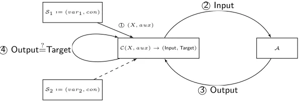
Our computational assumption is defined by the success probability among mul-tiple experiments, where each experiment is a sequence of interactions between a challengerCand an adversaryAas defined in Def. 5. In addition, we use a third party, the Source, denoted byS, who is responsible for generating the samples forC, as illustrated in Figure 1.
Definition 5 (Exp(C,A)). The experiment is defined as a sequence of interac-tions as follows:
1. S samples fromvar andconto obtain a sample(X, aux), and sends it to C; 2. C computes(Input,Target)← C(X, aux), and sendsInputto the A;
3. Areplies with a guessOutput.
The adversary wins the experiment if Target=Output.
We claim that the success probability ofAwill depend on three factors: a), the distribution of the source var; b) the distribution of theTarget; and c) the connection betweenInputandTarget, i.e., the combination ofCandA. Our goal is to ensure that, for varianceExpi, the success probability ofAiwill only depend on the distribution of the sourceSi. To achieve so, we use a same challengerC and adversaryApair throughout the experiments.
S1..= (var1, con)
S2..= (var2, con)
C(X, aux)→(Input,Target) A
1
(X, aux)
2 Input
3 Output 4
Output=Target?
Fig. 1.Data flow for our experiments
for sourceS1, then it cannot computeTargetfromX2for sourceS2. That is, the adversary cannot learn more information fromS1 than fromS2 for a fixedC.
Then, for any PPT challengerC, if the success probability of any adversary AinExp1 of Table 1 is negligible, so doesAinExp2.
Exp1(C,A) Exp2(C,A)
X1←var1 X2←var2
aux←con aux←con
Input1,Target1← C(X1, aux) Input2,Target2← C(X2, aux)
Output1← A(Input1) Output2← A(Input2)
Success ifOutput1=Target1 Success ifOutput2=Target2
Table 1.Exp1v.s. Exp2
To show that the above model is useful in a security proof, let us present a proof of an (informal) Diffie-Hellman version of the assumption within the above model. Looking ahead, we will use a similar approach to proof R-CLWR.
Definition 6 (The Diffie-Hellman analogue to our assumption). Let G
be a group. Let Zs be the distribution of (a, b) = (g, gs) where g ←$ G is a
randomly chosen group element and s is an randomly chosen and fixed index. Accordingly, letU be the distribution of(a, b) = (g, u)whereg, u←$G. Letvar1
denote the distribution Zl
s and var2 denote the distribution Ul. Let con be an
arbitrary distribution over{0,1}∗ which is independent ofvar
1 andvar2. For a
fixed PPT challengerC,P˚C(A)is the probability for a PPT adversaryAto win
the Exp1(C,A)with S1 in Table 1, whileQ˚C(A) is that forAto the Exp2(C,A)
with S2. Then, ifQ˚C is negligible for any PPT adversaryA, so isP˚C.
Game 1. TheInputforAis (gx, gy), and theTargetisgxy.
Game 2. TheInputforAis (u, gy) for some randomu, and theTargetisuy. Game 3. The Inputfor Ais (u, v) for some random uand v, and the Target is
wfor some randomw.
Observe that, in Game 3, u, v and w are independent, therefore the success probability of the adversary will be 1/|G|, which is negligible.
In the rest of the reduction, we will firstly proof the success probability of the adversary in Game 2 is also negligible. To meet the notation, we setvar1to be the distribution of ((a1, b1),(a2, b2)) for (a1, b1) = (g, gy) and (a2, b2) = (u, uy), and var2to be that for (a1, b1) = (g, v) and (a2, b2) = (u, w). Setconto be dummy. C is then defined as given X = ((a1, b1),(a2, b2)), compute Input= (a2, b1) and Target = b2. As per Def. 6, if the success probability of Exp2 in Table 2 is negligible, so is that ofExp1. Therefore, the success probability of the adversary in Game 2 is negligible.
Exp1(C,A) Exp2(C,A)
((g, gy),(u, uy))←var1 ((g, v),(u, w))←var2
Source ⊥ ←con ⊥ ←con
X1←((g, gy),(u, uy)),⊥) X2←(((g, v),(u, w)),⊥)
Challenger Input1←(u, g
y
) Input2←(u, v)
Target1←uy Target
2←w
Attacker Output1← A((u, g
y
)) Output2← A(u, v)
Success ifOutput1=uy Success ifOutput
2=w Table 2.Reduction between Game 2 and 3
Then we will proof the success probability of the adversary in Game 1 is also negligible. Let con be the distribution of choosing an arbitrary index y; var1 be the distribution of (a1, b1) for (a1, b1) = (g, gx); and var2 be that for (a1, b1) = (g, v). Accordingly,Cis defined as givenX = ((a1, b1), y) and computes Input= (b1, a
y
1) andTarget=b y
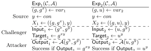
1. As per Def. 6, if the success probability ofExp2 in Table 3 is negligible, so is that ofExp1. Therefore, the success probability of the adversary in Game 1 is negligible.
Exp1(C,A) Exp2(C,A) (g, gx)←var1 (g, u)←var2
Source y←con y←con X1←((g, gx), y) X2←((g, u), y)
Challenger Input1←(g
x
, gy) Input2←(u, g
y ) Target1←gxy Target
2←u
y
Attacker Output1← A(g
x
, gy) Output2← A(u, g
y ) Success ifOutput1=gxySuccess ifOutput
2=u
y
In the next section, we will give more details on how to instantiate the frame-work as per Def. 6 where the underlying discrete log problem is replaced by a lattice problem.
4
The Computational Ring-LWR Assumption
For simplicity, we make use of the following additional notations. We refer to a uniformly distribution over [−β, β] asUβ. Accordingly, denote byUβnthe distri-bution overRq where each coefficient is no greater thanβ. For a distributionχ overK, we say ¯χis the discretization distribution overR, which is obtained by rounding each coefficient in the power basis to the nearest integer. For a distri-butionχ0 overR, denote by (χ0)×the distribution of the output of the following process: sample an element a← χ0, output a ifa is invertible; repeat until an output is obtained.
Now we are ready to give a formal definition of theR-CLWRassumption. This definition, as hinted in previous section, allows us to prove that an adversary cannot learn more information fromR-CLWR sample inputs than from uniform inputs. Our definition follows the framework of the Table 1. The only variation here is on the definitions ofvar1 andvar2.
Definition 7 (Computational Ring-LWR Assumption). Letq,pandl be positive integers. Fix an sthat is chosen from a distribution χ overR. Denote by Xs the distribution of (a,bascp)where a←$Rq; and denote by U the
distri-bution of (a,bbcp) where a, b ←$ Rq. Let Si = (vari, con), where var1 denotes
the distribution Xl
s; var2 denote the distribution Ul; and con is an arbitrary
distribution over {0,1}∗ which is independent from var
1 and var2. For a fixed
PPT challenger C, letPC,A(χ)be the probability for a PPT adversary Ato win
Exp1(C,A)withS1, whileQC,A be that for Ato winExp2(C,A)withS2.
The computational ring-LWR assumption with regard to a secret distribution
χ, denoted by R-CLWRp,q,l,χ, orR-CLWRχ for short, is that for any challenger C, ifQC,Ais negligible for any PPT adversaryA, so isPC,A.
Correspondingly, we also define thecomputational rounded learning with er-rors over the ring(R-CRLWE) assumption. Notice its difference from a computa-tionalLWEover the ring assumption, which, by the analogy toR-CLWR, replaces R-LWRsamples (bascp) withR-LWEsamples (as+e). By contrast, inR-CRLWE, one replacesR-LWRsamples withroundedR-LWEsamples (bas+ecp).
Definition 8 (Computational Ring-RLWE Assumption). Let q,p, l, s,
χandU be the same as Def. 7. Denote byYs,χ0 the distribution of(a,bas+ecp)
where a ←$ Rq and e ←χ0 over R. Let Si = (vari, con), where var1 denotes
the distributionYl
s,χ0;var2 denotes the distributionUl;condenotes an arbitrary
distribution over {0,1}∗ which is independent of var
1 and var2. For a fixed
PPT challenger C, let PC0,A(χ, χ0) be the probability for a PPT adversaryA to
Exp1(C,A)withS1, whileQC,A to be that for Ato winExp2(C,A)withS2.
is that for any challenger C, if QC,A is negligible for any PPT adversary A, so
isPC0,A(χ, χ0).
This definition suggests that the adversary cannot learn more information from R-CRLWEinputs than from uniform inputs. Next, we show that theR-CLWR as-sumption holds for uniform secrets, assuming the hardness of the decisional R-LWEassumption. Formally, we will have the following theorem.
Theorem 2 (Main Theorem). Following the notions in Def. 7 and Def. 8. For any ring R satisfying (3) and (5), the largest degree of the irreducible fac-tors modulo integer q of the polynomial f is less than kq. If l is a constant,
α ≥ c2c4
p
nln(2n)qkq/n·δK, β = Ω(nlα) and q/p = Ω(nlα/c
2c4), there is
a reduction from the decisional ring-LWE assumption R-LWEq,t·DH
α,t·DαH to the
computational ring-LWR assumption R-CLWRp,q,l,(Un β)×.
R-CLWR
(U nβ)× R-CLWR(U nβ+ ¯Dn α0)
× R-CRLWE
(U nβ+ ¯Dn α0)
×,Dn¯ α0
R-CRLWE
(U nβ+t·DHα)×,t·DHα R-LWE
(U nβ+t·DHα)×,t·DHα R-LWE
U nβ+t·DHα ,t·DHα R-LWE
t·DHα ,t·DHα
§4.1 §4.2 §4.3
§4.4
§4.5
§4.6
Fig. 2.Reduction flow fromR-LWEtoR-CLWR
Combing with the worst-case/average-case reduction in Theorem 1, the hard-ness of ourR-CLWRproblem will be based on the worse-case hardness of lattice problems. It is worth pointing out that, the majority of practical cryptosystems uses a cyclotomic ringR=Z[x]/(xn+ 1) wherenis a power of 2. For this ring, we have the following result.
Corollary 1. Following the same notations. For R = Z[x]/(xn+ 1) where n
is a power of 2, if l is a constant, α ≥ 2pnln(2n)·q2/n, β = Ω(nlα) and
q/p=Ω(n2lα), there is a reduction from the decisional ring-LWE assumptionR
-LWEq,t·DH
α,t·DHα to the computational ring-LWR assumption R-CLWRp,q,l,(U n β)×. 4.1 From R-CLWR(Un
β+ ¯Dnα0)× to R-CLWR(Uβn)×
We begin with proving the following lemma which shows the RD between the two distributions on Z, namelyUβ andUβ+ ¯Dα, is bounded by 1 + 1/n.
Lemma 6. Following the same notion. In addition, letUβ be a uniform distri-bution from [−β, β] over Z where β > α. Let the distribution ψ = ¯Dα+Uβ.
ThenRD2(Uβkψ)≤1 +cβα wherec= (1−exp(−π)) 2
Proof. Recall that the density function of ¯Dαis
f(i) = 1 α
Z 1/2 −1/2
exp
−π(i+x) 2 α2
dx.
By definition,
RD2(Uβkψ) = β
X
i=−β
1 (2β+1)2 1
2β+1
Pβ
j=−βf(i−j)
= 1
2β+ 1 β
X
i=−β
1
Pβ
j=−βf(i−j) .
For one dimensional standard Gaussian, we have the following tail bound [22]:
1 √ 2π Z ∞ z exp −x 2 2
dx≤1 2exp −z 2 2 . Therefore, β X
j=−β
f(i−j)
=1 α
Z β+1/2 −β−1/2
exp
−π(i+x) 2 α2
dx
=1−1 α
Z ∞
β+i+1 2 exp −πx 2 α2 dx+ Z ∞
β−i+1 2 exp −πx 2 α2 dx !
≤1−1 2exp
−π β+i+122
α2
!
−1 2exp
−π β−i+122
α2
!
.
Notice the symmetry:h(i) =h(−i). Define
t(x) :=1 2exp
−π(β+x+1
2) 2 α2 +1 2exp
−π(β−x+1
2) 2 α2
.
When 0≤x≤β, we take the maximum for both items independently and get an upper bound oft(x)
t(x)≤1
2exp −π
β+1 2
2
/α2
!
+1
2exp −π
1 2 2 /α2 ! ≤1
2exp −πβ 2/α2
+1 2 :=
1 2σα,β+
1 2,
(6)
whereσα,β = exp−παβ22
≤exp (−π). According to the mean value theorem of differentials, we have
g(t) := 1
1−t = 1 +g
0(ξ)t= 1 + t
for 0≤ξ≤t. Combining with the upper bound fort(x) in (6) when 0≤x≤β, we have
g(t(x))≤1 + 4·t(x) (1−σα,β)2. Therefore, we obtain
RD2(Uβkψ)
= 1
2β+ 1 β
X
i=−β
1
Pβ
j=−βf(i−j) ≤ 1
2β+ 1 β
X
i=−β g(i)
= 1
2β+ 1 β
X
i=0
g(i) + 1 2β+ 1
β
X
i=1
g(i) (sinceg(i) =g(−i))
≤ 1 2β+ 1
β
X
i=0
1 + 4
(1−σα,β)2 t(i)
+ 1
2β+ 1 β
X
i=1
1 + 4
(1−σα,β)2 t(i)
= 1 + 4
(1−σα,β)2(2β+ 1) β
X
i=−β
t(i) (sincet(i) =t(−i))
≤1 + 4α
(1−σα,β)2(2β+ 1) ≤1 + 2α
(1−exp (−π))2β
The second last inequality holds because
β
X
i=−β t(i) =
β
X
i=−β 1 2exp
−π(β+i+1 2) 2 α2 + β X
i=−β 1 2exp
−π(β−i+1 2) 2 α2 ≤ β X
i=−β
Z i+12
i−1 2
1 2exp
−π(β+x)2 α2
dx+ β
X
i=−β
Z i+12
i−1 2
1 2exp
−π(β−x)2 α2
dx
≤
Z β+12 −β−1
2 1 2exp
−π(β+x)2 α2
dx+
Z β+12 −β−1
2 1 2exp
−π(β−x)2 α2
dx
≤
Z +∞ −∞
1 2exp
−π(β+x)2 α2
dx+
Z +∞ −∞
1 2exp
−π(β−x)2 α2 dx ≤α. u t
Lemma 7. Following the same notation, ifβ =Ω(nlα),PC,A(Uβn)
2
≤2PC(Uβn+ ¯
Dn
α).Hence there is a reduction from R-CLWR(Un β+ ¯Dnα0)
× toR-CLWR(Un β)×.
Proof. Note thatPC,A((Uβn)×)
2
≤PC,A((Uβn+ ¯Dαn)×)·RD2 UβkUβ+ ¯Dα nl
.
Lemma 6 says RD2 UβkUβ+ ¯Dα
nl
≤2 whenβ =Ω(nlα). On the other hand, assuming the hardness ofR-CLWR(Un
β+ ¯Dαn)×, we have that for any challengerC, PC,A((Uβn+ ¯D
n
α)×) is negligible when QC,A is negligible. By the above result,
PC,A((Uβn)
×) is also negligible. So the assumptionR-CLWR
(Un
β)× holds. ut
4.2 From R-CRLWE(Un
β+ ¯D n α0)
×,D¯n α0
to R-CLWR(Un β+ ¯D
n α0)
×
The following lemma is adapted from [12] with a slight modification on the noise distribution. We provide a proof for completeness.
Lemma 8 ([12]). Assume B < q/2p. For every unit s ∈ Rq and noise
dis-tribution χ that is balanced over Rq and each coefficient is bounded by B with
probability larger than δ, we have RD2(XskYs)≤(1 + 2pB/q)n/δn whereXs is
the random variable (a,ba·scp)and Ys is the random variable (a,ba·s+ecp)
with a←Rq ande←χ.
Proof. By the definition,
RD2(XskYs) =Ea←Rq
P r(Xs= (a,ba·scp)) P r(Ys= (a,ba·s+ecp))
=Ea←Rq
1
Pre←χ(ba·s+ecp=ba·scp) .
We define the set borderp,q(B) = nx∈Zq :
x−
q pbxcp
< B
o
. For a ring element a∈Rq, we useai to denote theith coefficient in the power basis. For fixedsand for anyt∈[n], we define the set
BADs,t={a∈Rq :|{i∈[n],(a·s)i ∈borderp,q(B)}|=t}.
These are candidatea-s for whicha·shas exactly tcoefficients which are dan-gerously close to the rounding boundary. Fix an arbitrarytanda∈BADs,t. For anyi∈[n] such that (a·s)i∈/borderp,q(B), Prei[b(a, s)i+eicp=b(a, s)icp]≥δ. For any i∈[n] such that (a·s)i ∈borderp,q(B), we still haveb(a·s)i+eicp= b(a·s)icp as long as ei ∈ [−B, . . . ,0]. By the assumption on the noise distri-bution, we have Prei[b(a·s)i +eicp = b(a·s)icp] ≥ 1/2. Because e is inde-pendent over all coefficients and a has exactly t coefficients in borderp,q(B), Pre←χ(ba·s+ecp =ba·scp)≥ 21tδn−t≥
1 2tδn.
Sincesis a unit inRq,a·swill be uniform overRq and
Pr [a∈BADs,t]≤
n
t 1−
|borderp,q(B)| q
n−t|border
p,q(B)| q
t
Conditioning on the eventa∈BADs,t, we conclude
RD2(XskYs)≤δ−n n
X
t=0
2t·Pr[a∈BADs,t] =δ−n
1 + |borderp,q(B)| q
n
.
u t
Lemma 9. Adopt the same notions and symbols in Def. 7 and Def. 8. If p < q√π
2nlα√ln(2nl),we have PC,A(Uβn+ ¯D
n α)
×2
≤e2PC0,A (Uβn+ ¯Dnα0)×,D¯nα0.
Hence there is a reduction from R-CRLWE(Un β+ ¯D
n α0)
×,D¯n α0
toR-CLWR(Un β+ ¯D
n α0)
×.
Proof. We have
PC,A(Uβn+ ¯D n α)
2
≤PC0,A (U
n β + ¯D
n
α0)×,D¯αn0
·RD2(XskYs)l. Note that a one-dimensional GaussianDα overRsatisfies the tail bound
Pr x←Dα
[|x| ≥B]≤2 exp(−π(B/α)2)
for anyB≥0. We setB=
q
ln(2nl)
π α, so 2 exp(−π(B/α)
2)≤1/nlandδ≥1−1 nl. Also we setp < q/2nlB, then we have
RD2(XskYs)l≤(1 + 2pB/q)nl/δnl ≤
(1 + 1/nl)nl (1−1/nl)nl ≤e
2 (7)
AssumingR-CRLWE(Un β+ ¯D
n α0)
×
,D¯n α0
assumption holds, then for anyC andA,
PC0,A(Uβn+ ¯Dαn0)×,D¯nα0
is negligible so long asQC,Ais negligible. By the result
of (7), PC,A(Uβn+ ¯Dαn0)× is also negligible. This proves the R-CLWR(Un β+ ¯Dnα0)
×
assumption. ut
4.3 From R-CRLWE
(Un β+t·DHα)
× ,t·DH
α
to R-CRLWE
(Un β+ ¯D
n α0)
× ,D¯n
α0
Lemma 10. Following the same notations. Additionally, let t·DH
α be the
dis-cretization oft·DH
α, whereDαH is the continuous Gaussian with widthαover the H space. D¯αn0 is the discretization of the continuous Gaussian with widthα
ac-cording to the power basis.Y0
t·DH α,t·DHα
is the random variable(a,ba·s+ecp)with
a←$Rq ands, e←t·DαH, andYD0¯n α0,
¯ Dn
α0
is the random variable(a,ba·s+ecp)
with a←$Rq ands, e←D¯nα0. For any ringRsatisfying (3) and (5), when
α/c1c3≤α0 ≤
1 + 1 n
τ1+τ2
α/c2c4,
we have
RD∞
Y0 t·DH
α,t·DαH kYD0¯n
α0,D¯αn0
Proof. According to the data processing inequality of R´enyi divergence, it is suf-ficient to showRD∞ Dnαkt·DHα
≤eτ1+τ2.So we need to prove for allx∈
Rn,
ρ(x)/ρ0(x)≤eτ1+τ2. Recall thatt·DH
α has the probability density function over the power basisρ(x) = (αndet(D) det(B))−1exp−πxT D−1TΣ−1D−1x/α2, and Dn
α has the probability density function over the power basis ρ0(x) = α0−nexp −πxTx/α02
.Hence,
ρ(x) ρ0(x) =
α0n
αndet(D) det(B)exp π xTx
α02 −
xT D−1TΣ−1D−1x α2
!!
.
According to (2) and (4),Σ =BTB, kD−1xk ≥c1kxk for anyx∈
Rn and
kB−1yk ≥c3kykfor anyy∈
Rn. Ifα0 ≥α/c1c3, we have xT D−1T
Σ−1D−1x
α2 ≥
c21c23xTx
α2 ≥
xTx α02 . Therefore,
ρ(x) ρ0(x) ≤
α0n
αndet(D) det(B) ≤e τ1+τ2
whenα0 ≤ 1 + n1τ1+τ2
αc2c4≤ 1 +n1 τ1+τ2
α|det(D)|1/n|det(B)|1/n. Accord-ing to (3) and (5), we have c2≤ 1 +n1
τ1
c1 andc3 ≤ 1 + 1n
τ2
c4. Therefore there must exist at least anα0 that satisfiesα/c
1c3≤α0≤ 1 +n1
τ1+τ2
α/c2c4. u t
Lemma 11. Adopt the same notions and symbols as above. For any ring R
satisfying (3) and (5), when α/c1c3 ≤ α0 ≤ (1 + 1/n)
τ1+τ2α/c
2c4, we have PC0,A
Un
β +t·DHα
×
, t·DH α
≤ el(τ1+τ2)P0
C,A
Un β + ¯D
n α
×
,D¯n α
. Hence
there is a reduction fromR-CRLWE
(Un β+t·DαH)
×
,t·DH α
toR-CRLWE
(Un β+ ¯Dαn0)
×
,D¯n α0
.
4.4 From R-LWE(Un
β+t·DHα)×,t·DαH
to R-CRLWE(Un
β+t·DHα)×,t·DHα
Lemma 12. Adopt the same notions and symbols in Def. 7 and Def. 8. As-sume the advantage of any probabilistic polynomial time algorithm to solve the decisional R-LWE problem R-LWE(Un
β+t·DHα)×,t·DHα
is less than ε, then we have
PC0,A
Un
β +t·DHα
×
, t·DH α
−QC,A
< εfor any PPT adversary A.
corresponding Input and Target. B also check whether the Output of A equals theTarget. If the check is passed,Boutputs 1; otherwise it outputs 0.
When (x1, y1), . . . ,(xl, yl) areR-LWEsamples,
Pr(B((x1, y1), . . . ,(xl, yl)) = 1) =PC0,A
Uβn+t·DH α
×
, t·DH α
;
by contrast, when (x1, y1), . . . ,(xl, yl) are uniform samples, Pr (B((x1, y1), . . . ,(xl, yl)) = 1) =QC,A
for adversaryA. Thus, assuming the hardness of decisional ring-LWE, we have
PC0,A
Un
β +t·DHα
×
, t·DH α
−QC,A
< εfor negligibleε.
u t
4.5 From R-LWEUn
β+t·DαH,t·DαH to R-LWE(Uβn+t·DHα)×,t·DHα Lemma 13. LetDn
ˆ
α be a continuous Gaussian with widthαˆ andDαH be a
con-tinuous Gaussian overH with widthα. Lett=f0(ζ). If the assumption (3) and (5) holds, when (1+1/n)τα1 +τ2c1c3 ≤αˆ≤
α
c2c4,we haveRD∞(D n ˆ α|t·D
H α)≤e
τ1+τ2. The proof is similar to Lemma 10. We omit the details and recommend readers to refer the full version [19].
Lemma 14. LetDn ˆ
αbe a continuous Gaussian distribution overKRwhereK∼=
Q[X]/(f(X)). The largest degree of the irreducible factors modulo integer q of
the polynomial f is less than kq. Let αˆ ≥
p
nln(n/ε)qkq/n·δ
K and β is any
positive integer. If a←Un β +D
n ˆ
α, the probability of that ais invertible is larger
than1−q−kq−ε.
Proof. Our goal is to bound the probability thatais inI :=hq, φibyq−n/kq+ε, for any k ≤ kq, when a ← Uβn +Dn
ˆ
α. Specifically, denote a := a1+a2 where a1 ←Uβn and a2 ← Dαnˆ. We have N(I)≥ q
kq. By Minkowski’s theorem, this implies λ1(I) ≤
√
nqkq/n. Since I is an ideal of R, we have λn(I) = λ 1(I). Then, in Lemma 2, we have λn(I)≤√nqkq/n·δK, and in Lemma 3, we have ηε(I) ≤p
ln(n/ε)λn(I) ≤p
nln(n/ε)qkq/n·δK. In addition, Lemma 4 shows that the statistical distance betweenbmodI and a uniform distribution modulo I is less thanεforb←Dn
ˆ
α. Sincea1=bbe ∈RandI ⊆R,a1will be uniform in RmodI with a statistical distanceε. This implies thata=a1+a2 is uniform inRmodI with statistical distanceε. So we havea= 0 modI with probability less than q−kq+ε. When we setε= 1/2, we get the desired result. ut
Lemma 15. Following the above notations. For any ringR satisfying (3) and (5), whenα≥c2c4
p
nln(2n)q2/n·δ
K, there is a reduction fromR-LWEUn
β+t·DHα,t·DαH
toR-LWE
(Un β+t·DHα)
×
,t·DH α
Proof. Let Pr(AOχ,s = 1) = p
0(s), Pr(AU(Rq×Rq) = 1) = p1 and the set Sε denote the allsthat|p0(s)−p1|> εfor any non-negligibleε, then we have
Prs∈Sε|s←Uβn+t·DαH
= Pr
s∈Sε|s←Uβn+t·DH α
×
Prs∈R×q|s←Uβn+t·DH α
+ Pr s∈Sε|s←Uβn+ ¯D H
αand output whensnot invertible
Pr sis not invertible|s←Uβn+ ¯DHα
≥Pr
s∈Sε|s←Uβn+t·DH α
×
Prs∈R×q|s←Uβn+t·DH α
.
Next, Lemma 13 says for (1+1/n)τα1 +τ2c1c3 ≤αˆ ≤ α c2c4,
Prs∈R×q |s←Uβn+t·DH α
≥
Prs∈R×q|s←Un β +D
n ˆ α
RD∞(Dnαˆkt·DHα)
≥
Prs∈R×q|s←Uβn+Dαnˆ
exp(τ1+τ2) In addition, in Lemma 14 we have proved Prs∈R×q|s←Uβn+Dn
ˆ α
is
non-negligible for ˆα≥p
nln(n/ε)qkq/n·δK. So Prs∈R×
q |s←Uβn+t·DHα
is also
non-negligible. This implies Prs∈S|s←Uβn+t·DH α
is non-negligible as long
as Pr
s∈S|s←Un
β +t·DαH
×
is also non-negligible, i.e. an adversary can
solveR-LWEUn
β+t·DαH,t·DHα
so long as it can solveR-LWE (Un
β+t·DHα)
×
,t·DH α
. ut
4.6 From R-LWEt·DH α,t·DHα
to R-LWEUn
β+t·DαH,t·DαH
Lemma 16. Letψ=t·DH
α +Uβn be a distribution. If there is a PPT algorithm A0 that distinguishes O
s,χ from U within m queries for s←ψ, then there is a
PPT algorithm A which distinguishes Os,χ from U within m queries for s ← t·DH
α.
Proof. Given m elements (ai, bi) ∈ Rq ×Rq, drawn from either Os,Dα¯
m
for s ← t·DH
α, or (U(Rq×Rq)) m
, the reduction algorithm chooses s0 ← Uβn and outputsmelements (ai, bi+ais0)∈Rq×Rq. Obviously, when (ai, bi) are drawn fromOs,D¯α, (ai, bi+ais
0) are drawn fromO
s+s0,D¯α and the distribution ofs+s
0
will beψ=t·DH
α+Uβn. When (ai, bi) are all drawn fromU(Rq×Rq), (ai, bi+ais0)
5
Application I: A Public Key Encryption
In this section, we will provide an IND-CPA securePKE scheme based on the R-CLWR assumption. Our scheme improvesR-LWE based schemes in both time and space efficiency. At a high level, our scheme uses the standard KEM-DEM approach, where the KEM, similar to that of [54], stems from an IND-CPA secure scheme.
5.1 Reconciliation Mechanism.
Reconciliation was firstly proposed by [26], and has a few variants, for example, [54, 3]. In this paper, for the ease of presentation, we will follow the work of [54].
Let us define the reconciliation rounding function as [·]2,q:x→j2 q ·x
k
mod
2, and the reconciliation cross-rounding function as h·i2,q : x→ j4 q ·x
k
mod 2. Then the algorithm Rec will be defined as follows. On input y ∈ Zq and z ∈ {0,1}, Rec(y, z) outputs [x]2,q, where x is the closest element toy such that hxi2,q =z. First, whenqis even, we have following results.
Lemma 17. If x∈ Zq is uniformly random, [x]2,q is uniformly random given hxi2,q.
Lemma 18. If|x−y|< q/8, then we have Rec(y,hxi2,q) = [x]2,q.
On the other hand, when the modulusqis odd, we make use of a randomized doubling function: letDbl:Zq →Z2q, x7→Dbl(x) = 2x−e, whereeis sampled from {−1,0,1} with probabilities p−1 =p1 = 1/4 and p0 = 1/2. We have two similar lemmas.
Lemma 19. For oddq, ifx∈Zq is uniformly random andx¯←$Dbl(x), then [¯x]2,2q is uniformly random given hx¯i2,2q.
Lemma 20. For oddq , let|x−y|< q/8 forx, y∈Zq. Let x¯=Dbl(x). Then Rec
y,hx¯i2,2q= [¯x]2,2q.
Moreover, the above reconciliation mechanism can be extended coefficient-wise toRq with respect to the power basis.
5.2 PKE Schemes
Ring-LWE Based PKE. Let H : {0,1}n → {0,1}k be a hash function for integer k. G : {0,1}k0 → R
q be a pusedorandom generator. The R-LWE based scheme consists of the following three algorithms.
– RLWE.KeyGen(1λ): Given the security parameterλ, chooseseed← {0,1}k0, a=G(seed)∈Rqands, e1←t·DHα. Output (seed, b=sa+e1)∈ {0,1}k
0
× Rq as the public key andsas the secret key.
– RLWE.Encryption(pk= (seed, b),m∈ {0,1}k): Given the messagem, choose r, e2, e3←t·DαH. Compute ˆv=br+e2andv=hDbl(ˆv)i2,2q. Also compute a=G(seed),u=ra+e3 and w=H([Dbl(ˆv)]2,2q)⊕m. The ciphertext is ct= (u, v, w)∈Rq× {0,1}n× {0,1}k.
– RLWE.Decryption(ct = (u, v, w), sk = s): Compute v0 = su and output m0=w⊕ H(Rec(v0, v)).
Correctness. In fact, ˆv=br+e2= (as+e1)r+e2=asr+ (e1r+e2) and v0= su= (ar+e3)s=asr+se3.Suppose each coefficient ofe1, e2, e3, r, sis bounded byB with overwhelming probability, we have|e2r+e1| ≤nB2+B and|se3| ≤ nB2. To ensure correctness, we need to make sure|vˆ−v0|< q/8, hence we require
2nB2+B < q/8. (8)
Ring-CLWR Based PKE. Next, we describe theR-CLWRversion of the above scheme. Firstly, as mentioned in the§1.1, we make use of a probabilistic function Inv(·) :Zp→Zq that takesx∈Zp as input and uniform randomly chooses an element from the set {u ∈ Zq|bucp=x} as the output. Apparently, we have bInv(bxcp)cp =bxcp and Inv(bxcp) is uniform in Zq when xis uniform inZq. We extend Inv(·) coefficient-wisely toRq with respect to the power basis. Also note that both Inv(·) and its extension to Rq are polynomial time algorithms. so long asp,qandnare of polynomial size.
– RCLWR.KeyGen(1λ): Given the security parameterλ, choose aseed← {0,1}k0
and a=G(seed)∈ Rq. Then, samples from (Uβn)× by repeating s← Uβn untilsis invertible. Output (seed, b=bsacp) as the public key andsas the secret key.
– RCLWR.Encryption(pk= (seed, b),m∈ {0,1}k): Given a messagem, sample r from (Uβn)× by repeating r ← Uβn until r is invertible. Compute ¯v = bInv(b)rcp, ˆv =Inv(¯v) andv =hDbl(ˆv)i2,2q. Also compute a= G(seed), u=bracp andw=H([Dbl(ˆv)]2,2q)⊕m. The ciphertext is ct= (u, v, w)∈ Rp× {0,1}n× {0,1}k.
– RCLWR.Decryption(ct= (u, v, w),sk=s): Computev0 =s
Inv(u) and out-putm0=w⊕ H(Rec(v0, v)).
Correctness. To show the correctness of the scheme, we need to make sure |vˆ−v0|< q/8. Specifically, we have
ˆ
and
v0 =sInv(u) = (ar+e3)s=asr+se3. When the secret is drawn from a uniform distribution Un
β, we have|e1| ≤q/p, |e2| ≤q/p |e3| ≤ q/p, |r| ≤β, |s| ≤β. We have |e2r+e1| ≤nβq/p+q/p and |se3| ≤nβq/p, hence we require
2nβq/p+q/p < q/8. (9)
5.3 Security Proof
In this subsection, we prove the IND-CPA security of the abovePKEbased on R-CLWR assumption as per Def. 7.
First, we will reduce the IND-CPA security to searching the pre-image of a hash function Hthrough the following Game.
1. The challengerC gives the adversaryAthe public keypk.
2. Achooses two messagesm0 andm1 and gives them to the challenger. 3. Cchooses a random bitb and givesAa ciphertext ctb that encryptsmb. 4. The adversaryAoutputs a bitb0 as a guess ofb.
SinceHis modeled as a random oracle, the adversaryAwill successfully guess the bitbwith probability 1/2, unless he has previously queried the value [Dbl(ˆv)]2,2q corresponding to the challenge ciphertext to the random oracle. Therefore, we can construct an adversaryA0fromA, which, upon inputting the public keypk
and (u, v)∈Rp× {0,1}n, outputs the value [
Dbl(ˆv)]2,2q. In a bit more details, whenA0 receivespkand (u, v)∈Rp× {0,1}n, it returnspk toA. WhenA gen-erates the message pair (m0, m1),A0 choosesr← {0,1}n,b← {0,1} and sends Athe ciphertexts (u, v, mb⊕r). In the meantime, A0 answers theHqueries of
A by keeping a random oracle table. Since we have assumed that A success-fully guesses the bitbwith a non-negligible advantage, the value of [Dbl(ˆv)]2,2q must be queried by A with a non-negligible probability. Consequently,A0 can successfully output the value [Dbl(ˆv)]2,2q with a non-negligible probability.
Next, we will show that the success probability ofA0 is negligible under the
R-CLWRassumption. Specifically, we can construct following games.
Game 1. Choose a ← Rq and s, r ← (Uβn)×. b = bsacp, ¯v = bInv(b)rcp, ˆv = Inv(¯v), v = hDbl(ˆv)i2,2q and u = bracp. A0 is given (u, v) and its target is to compute [Dbl(ˆv)]2,2q.
Game 2. Choose a ← Rq and s, r ← (Un
β)×. b ← U(bRqcp), ¯v = bInv(b)rcp, ˆ
v=Inv(¯v),v=hDbl(ˆv)i2,2q andu=bracp.A0 is given (u, v) and its target is to compute [Dbl(ˆv)]2,2q.
Game 3. Choose a← Rq and s, r ← (Uβn)×. c ← Rq, ¯v = bcrcp, ˆv = Inv(¯v), v=hDbl(ˆv)i2,2q andu=bracp. A0 is given (u, v) and its target is to compute [Dbl(ˆv)]2,2q.
Game 4. Choosea←Rqands, r←(Un
Firstly, we definevar1,var2,con andC as follows. We set conas the distri-bution of choosing r from (Un
β)
×. Let var
1 be the distribution of (a, b) where b = bsacp and var2 be the distribution of (a, b) where b ← U(bRqcp). The challengerCcomputesInput= (bracp,hDbl(Inv(bInv(b)rcp))i2,2q) = (u, v) and Target = [Dbl(Inv(bInv(b)rcp))]2,2q. According to the R-CLWR assumption, if the success probability for anyAis negligible when b← U(bRqcp), that is also negligible when (a, b) is an R-LWRinstance. Therefore, the success probability of Game 1 is negligible if that of Game 2 is negligible.
Secondly, the success probability of Game 2 and that of Game 3 are same, sinceInv(b) is uniform inRq forb← U(bRqcp), and the views and the goals of the adversary in both games remain the same.
Thirdly, we definevar1,var2,conandCas follows. We setconto be dummy. Let var1 be the distribution of ((c,v),¯ (a, u)) where ¯v =bcrcp and u=bracp, while S2 to be the distribution of ((c,v),¯ (a, u)) where ¯v, u ← U(bRqcp). The challengerC computes theInput= (u,hDbl(Inv(¯v))i2,2q) = (u, v) andTarget= [Dbl(Inv(¯v))]2,2q.
According to theR-CLWRassumption, if the success probability for anyAis negligible when ¯v, u← U(bRqcp), then that is also negligible when ((c,v),¯ (a, u)) is anR-LWRinstance. Therefore, the success probability of Game 3 is negligible if that of Game 4 is negligible.
Finally,uand ¯v are independent in Game 4. Since ¯v← U(bRqcp),Inv(¯v) is uniform inRq. According to Lemma 19, [Dbl(Inv(¯v))]2,2q is uniformly random givenhDbl(Inv(¯v))i2,2q, so the success probability of Game 4 is negligible.
Combining all above analyses, we conclude that the success probability of A0 in Game 1 is negligible under theR-CLWR assumption. In other words, the
R-CLWR basedPKEscheme is IND-CPA secure.
5.4 Parameters and Comparisons
Time Complexity. As discussed in the introduction, the sampling subroutine is usually the most intricate part during the implementations. In anR-LWEbased scheme, one needs to produce two samplings during the key generation and three samplings during the encryption. In comparison, in an R-CLWR based scheme, one only needs to proceed a single sampling for each key generation and encryption. Moreover, an R-LWE based scheme needs to sample from rounded Gaussian, while we can simply sample uniformly from a small interval and reject when it is non-invertible for anR-CLWRbased scheme.
In terms of efficiency, we believe that our sampling subroutine will be much more efficient for the following reasons. First, it allows us to save a huge amount of entropy in practice. Secondly, and more importantly, a single sampling routing becomes more efficient in our case as we only require uniform sampling.
meantime, the invertibitiy check for a ring element can be carried out efficiently through the extended GCD algorithm.
Lemma 21. LetDn
αbe a continuous Gaussian distribution overKRwhereK∼=
Q[X]/(f(X)). The largest degree of the irreducible factors modulo integer q of
the polynomialf is less than kq. Let αˆ ≥p
nln(n/ε)qkq/n·δK andβ >3nˆα. If b←Uβn, the probability of thatbis invertible is larger than1−2q−kq−2ε.
Proof. According to Lemma 14, when a ← Uβn+Dn ˆ
α, the probability of that ais non-invertible is smaller thanq−kq +ε. According to Lemma 6, RD
2(Uβn k Un
β +Dnαˆ) =RD2(UβkUβ+Dα)ˆ
n ≤2.So
Pr(bis non-inv)≤Pr(ais non-inv)·RD2 UβnkU n β +Dnαˆ
≤2q−kq+ 2ε. ut
Space Complexity. Next, we will choose the parameters for these two schemes to deliver a fair comparison. As motivated in the introduction, we aim to keep decryption failure probability less thanO(1/en).
For the R-LWE based scheme, as per average-case/worst-case reduction in Theorem 3, α=Ω(n1/4log1/4n). SinceR =
Z[x]/(xn+ 1), we havec1=c2= 1/√n,c3=c4= 1/n. Sincet=n·ζn−1, each coefficient of the error fromt·DαH is one-dimensional rounded Gaussian with width α0 =n1.5α, which is smaller than B =Ω(n0.5α0) =Ω(n0.5α/c2c4) =Ω(n2.25log1/4n) with probability 1− O(e−n). To make sure that (8) holds with probability 1−O(e−n), we must choose q=Ω(n5.5log0.5n). If we setq=n5.5log0.5n, the public key has size of k0+nlog(q) =k0+ 2.75·nlognand the ciphertext has size ofk+n+nlog(q) = k+n+ 2.75·nlogn.
For theR-CLWRbased scheme with uniform secret, according to the reduc-tions, β = Ω(nα0) = Ω(n2.75log1/4n) and q/p = Ω(n2.75log0.75n). To make sure that (9) holds with overwhelming probability, we can chooseq=n6.5logn andp=n3.75log1/4n. That results in the public key of sizek0+nlog(p) =k0+
0.9375·nlognand the ciphertext of sizek+n+nlog(p) =k+n+ 0.9375·nlogn.
6
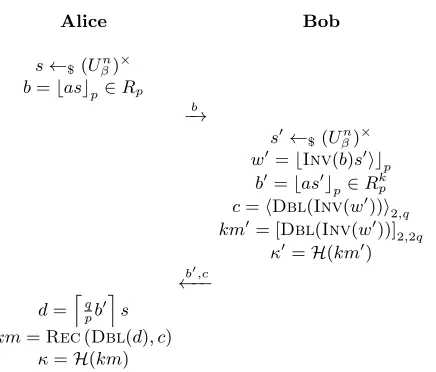
Application II: Diffie-Hellman type Key Exchange
For completeness, we also describe a key exchange protocol based onR-CLWRwith binary secret. The protocol is described in Table 4. Alice and Bob previously share the public ring elementa∈Rq. For every new exchange instance, Alice and Bob generate their secret ring elements s, s0 respectively, which are uniformly over (Un
β)×.κandκ0 are the session key which are finally acquired by Alice and Bob respectively.
Alice Bob
s←$(Uβn) ×
b=bascp∈Rp b −→
s0←$(Uβn) ×
w0=bInv(b)s0icp
b0=bas0cp∈Rk p
c=hDbl(Inv(w0))i2,q
km0= [Dbl(Inv(w0))]2,2q
κ0=H(km0) b0,c
←−−
d=lqpb0ms km=Rec(Dbl(d), c)
κ=H(km)
Table 4.A key exchange protocol based onR-CLWR.
7
Application III: New proofs for variant schemes
In this section, we will prove the IND-CPA security of a variant of Saber and Round2, under the R-CLWR assumption, for proper parameters and distribu-tions. Below we give an asymptotic simplification of their algorithms. There are two differences between the scheme to be presented andSaber/Round2. First, our scheme does not encrypt the messagem directly, instead, we encrypt a bit stringgand maskmby a one-time pad. Second, during the encryption, we lifted b toRq before multiplying it byrand rounding. These two modifications make the scheme suitable for our computational assumption.
Theorem 3. The simplified Round2 and Saber scheme is IND-CPA secure un-der the R-CLWR assumption R-CLWRp,q,1,χ andR-CLWRp,q,2,χ0 under the
ran-dom oracle model.
The proof is similar to subsection 5.3, and please refer to the full version [19]. Similarly, we can prove the IND-CPA security of the PKE scheme of the ring version of Lizard under R-LWE and R-CLWR, for proper parameters and distributions. We also need an asymptotic simplification of the algorithm that is similar to the scheme in previous subsection.
Theorem 4. The simplified Lizard scheme is IND-CPA secure under the ring-CLWR assumption R-LWEq,χ andR-CLWRp,q,2,χ0 in the random oracle model.
The proof can be found in the full version [19].