Localist representation can improve efficiency for detection and counting

Behavioral and Brain Sciences

Additional services for 

Behavioral and Brain Sciences:

Email alerts: Click here

Subscriptions: Click here

Commercial reprints: Click here

Terms of use : Click here

Localist representation can improve efficiency for detection and counting

Horace Barlow and Anthony Gardner­Medwin

Behavioral and Brain Sciences / Volume 23 / Issue 04 / August 2000, pp 467 ­ 468 DOI: 10.1017/S0140525X00223352, Published online: 09 February 2001

Link to this article: http://journals.cambridge.org/abstract_S0140525X00223352

How to cite this article:

Horace Barlow and Anthony Gardner­Medwin (2000). Localist representation can improve efficiency for detection and counting.  Behavioral and Brain Sciences,23, pp 467­468 doi:10.1017/S0140525X00223352

Request Permissions : Click here

1. Introduction

The aim of this target article is to demonstrate the power,

flexibility, and plausibility of connectionist models in

psy-chology which use localist representations. I will take care

to define the terms “localist” and “distributed” in the

con-text of connectionist models and to identify the essential

points of contention between advocates of each type of

model. Localist models will be related to some classic

math-ematical models in psychology and some of the criticisms of

localism will be addressed. This approach will be contrasted

with a currently popular one in which localist

representa-tions play no part. The conclusion will be that the localist

approach is preferable whether one considers

connection-ist models as psychological-level models or as models of the

underlying brain processes.

At the time of writing, it is thirteen years since the

pub-lication of Parallel Distributed Processing: Explorations in

the Microstructures of Cognition

(Rumelhart, McClelland,

& the PDP Research Group 1986). That two-volume set

has had an enormous influence on the field of

psychologi-cal modelling (among others) and justifiably so, having

helped to revive widespread interest in the connectionist

enterprise after the seminal criticisms of Minsky and Papert

(1969). In fact, despite Minsky and Papert’s critique, a

num-ber of researchers (e.g., S. Amari, K. Fukushima, S.

Gross-berg, T. Kohonen, C. von der Malsburg) had continued to

develop connectionist models throughout the 1970s, often

in directions rather different from that in which the 1980’s

“revival” later found itself heading. More specifically, much

of the earlier work had investigated networks in which

lo-calist representations

played a prominent role, whereas, by

contrast, the style of modelling that received most attention

as a result of the PDP research group’s work was one that

had at its centre the concept of distributed representation.

It is more than coincidental that the word “distributed”

found itself centrally located in both the name of the

re-search group and the title of its major publication but it is

important to note that in these contexts the words

“paral-lel” and “distributed” both refer to processing rather than

to representation. Although it is unlikely that anyone would

deny that processing in the brain is carried out by many

dif-ferent processors in parallel (i.e., at the same time) and that

such processing is necessarily distributed (i.e., in space), the

logic that leads from a consequent commitment to the idea

of distributed processing,

to an equally strong commitment

to the related, but distinct, notion of distributed

represen-tation,

is more debatable. In this target article I hope to

show that the thoroughgoing

use of distributed

representa-tions, and the learning algorithms associated with them, is

very far from being mandated by a general commitment to

parallel distributed processing.

As indicated above, I will advocate a modelling approach

that supplements the use of distributed representations

(the existence of which, in some form, nobody could deny)

with the additional use of localist representations. The

lat-ter have acquired a bad reputation in some quarlat-ters. This

cannot be directly attributed to the PDP books themselves,

in which several of the models were localist in flavour (e.g.,

Printed in the United States of America

Connectionist modelling in

psychology: A localist manifesto

Mike Page

Medical Research Council Cognition and Brain Sciences Unit, Cambridge, CB2 2EF, United Kingdom

[email protected] www.mrc-cbu.cam.ac.uk/

Abstract:Over the last decade, fully distributed models have become dominant in connectionist psychological modelling, whereas the virtues of localist models have been underestimated. This target article illustrates some of the benefits of localist modelling. Localist models are characterized by the presence of localist representations rather than the absence of distributed representations. A general-ized localist model is proposed that exhibits many of the properties of fully distributed models. It can be applied to a number of prob-lems that are difficult for fully distributed models, and its applicability can be extended through comparisons with a number of classic mathematical models of behaviour. There are reasons why localist models have been underused, though these often misconstrue the lo-calist position. In particular, many conclusions about connectionist representation, based on neuroscientific observation, can be called into question. There are still some problems inherent in the application of fully distributed systems and some inadequacies in proposed solutions to these problems. In the domain of psychological modelling, localist modelling is to be preferred.

Keywords: choice; competition; connectionist modelling; consolidation; distributed; localist; neural networks; reaction-time

interactive activation and competition models, competitive

learning models). Nonetheless, the terms “PDP” and

“dis-tributed” on the one hand, and “localist” on the other, have

come to be seen as dichotomous. I will show this apparent

dichotomy to be false and will identify those issues over

which there is genuine disagreement.

A word of caution: “Neural networks” have been applied

in a wide variety of other areas in which their plausibility as

models of cognitive function is of no consequence. In

crit-icizing what I see to be the overuse (or default use) of fully

distributed networks, I will accordingly restrict discussion

to their application in the field of connectionist modelling

of cognitive or psychological function. Even within this

more restricted domain there has been a large amount

writ-ten about the issues addressed here. Moreover, it is my

im-pression that the sorts of things to be said in defence of the

localist position will have occurred independently to many

of those engaged in such a defence. I apologize in advance,

therefore, for necessarily omitting any relevant references

that have so far escaped my attention. No doubt the BBS

commentary will set the record straight.

The next section will define some of the terms to be used

throughout this target article. As will be seen, certain

sub-tleties in such definitions becloud the apparent clarity of

the localist/distributed divide.

2. Defining some terms

2.1. Basic terms

Before defining localist and distributed representations, we

establish some more basic vocabulary. In what follows, the

word nodes

will refer to the simple units out of which

con-nectionist networks have traditionally been constructed. A

node might be thought of as consisting of a single neuron

or a distinct population of neurons (e.g., a cortical

minicol-umn). A node will be referred to as having a level of

acti-vation, where a loose analogy is drawn between this

activa-tion and the firing rate (mean or maximum firing rate) of

a neuron (population). The activation of a node might lead

to an output signal’s being projected from it. The projection

of this signal will be deemed to be along one or more

weighted connections, where the concept of weight in

some way represents the variable ability of output from one

node to affect processing at a connected node. The

rela-tionship between the weighted input to a given node (i.e.,

those signals projected to it from other nodes), its

activa-tion, and the output which it in turn projects, will be

sum-marized using a number of simple, and probably familiar,

functions. All of these definitions are, I hope, an

uncontro-versial statement of the basic aspects of the majority of

con-nectionist models.

2.2. Localist and distributed representations

The following definitions, drawn from the recent literature,

largely capture the difference between localist and

distrib-uted representations [see also Smolensky: “On the Proper

Treatment of Connectionism” BBS

11(1) 1988; Hanson &

Burr: “What Connectionist Models Learn” BBS

13(3) 1990;

Van Gelder: “The Dynamical Hypothesis in Cognitive

Sci-ence” BBS

21(5) 1998; O’Brien & Opie: “A Connectionist

Theory of Phenomenal Experience” BBS

22(1) 1999].

First, distributed representations:

Many neurons participate in the representation of each mem-ory and different representations share neurons. (Amit 1995, p. 621)

The model makes no commitment to any particular form of representation, beyond supposing that the representations are distributed; that is, each face, semantic representation, or name is represented by multiple units, and each unit represents mul-tiple faces, semantic units or names. (Farah et al. 1993, p. 577)

The latter definition refers explicitly to a particular model

of face naming, but the intended nature of distributed

rep-resentations in general is clear. To illustrate the point,

sup-pose we wished to represent the four entities “John,”

“Paul,” “George,” and “Ringo.” Figure 1a shows distributed

representations for these entities. Each representation

in-volves a pattern of activation across four nodes and,

impor-tantly, there is overlap between the representations. For

in-stance, the first node is active in the patterns representing

both John and Ringo, the second node is active in the

pat-terns representing both John and Paul, and so on. A

corol-lary of this is that the identity of the entity that is currently

represented cannot be unambiguously determined by

in-specting the state of any single node.

Now consider the skeleton of a definition of a localist

rep-resentation, as contrasted with a distributed coding:

With a local representation, activity in individual units can be interpreted directly . . . with distributed coding individual units cannot be interpreted without knowing the state of other units in the network. (Thorpe 1995, p. 550)

For an example of a localist representation of our four

en-tities, see Figure 1b. In such a representation, only one

node is active for any given entity. As a result, activity at a

given unit can unambiguously identify the currently

repre-sented entity.

When nodes are binary (i.e., having either activity 1 or 0),

these definitions are reasonably clear. But how are they

af-fected if activity can take, for example, any value between

these limits? The basic distinction remains: in the localist

model, it will still be possible to interpret the state of a given

node independent of the states of other nodes. A natural

way to “interpret” the state of a node embedded in a

local-ist model would be to propose, as did Barlow (1972), a

mo-notonic mapping between activity and confidence in the

presence of the node’s referent:

The frequency of neural impulses codes subjective certainty: a high impulse frequency in a given neuron corresponds to a high degree of confidence that the cause of the percept is present in the external world. (Barlow 1972, p. 381)

It may be that the significance of activating a given node is

assessed in relation to a threshold value, such that only

su-perthreshold activations are capable of indicating nonzero

confidence. Put another way, the function relating

activa-tion to “degree of confidence” would not necessarily be

lin-ear, or even continuously differentiable, in spite of being

monotonic nondecreasing.

Having offered both Thorpe’s and Barlow’s descriptions

of localist representation, I must point out that interpreting

a node’s activation as “degree of confidence” is potentially

inconsistent with the desire to interpret a given node’s

acti-vation “directly,” that is, independent of the actiacti-vation of

other nodes. For example, suppose, in a

continuous-activa-tion version of Figure 1b, that two nodes have near

maxi-mal activity. In some circumstances we will be happy to

re-gard this state as evidence that both the relevant referents

are present in the world: in this case the interpretation of

the node activations will conform to the independence

as-sumption. In other cases, we might regard such a state as

indicating some ambiguity as to whether one referent or the

other is present. In these cases it is not strictly true to say

that the degree of confidence in a particular referent can be

assessed by looking at the activation of the relevant node

alone, independent of that of other nodes. One option is to

assume instead that activation maps onto relative

degree of

confidence, so that degree of activation is interpreted

rela-tive to that of other nodes. Although strictly inconsistent

with Thorpe’s desire for direct interpretation, this preserves

what is essential about a localist scheme, namely that the

entity about which relative confidence is being expressed is

identified with a single node. Alternatively, both Thorpe’s

and Barlow’s definitions can be simultaneously maintained

if some competitive process is implemented directly (i.e.,

mechanically), so that it is impossible to sustain

simultane-ously high activations at two nodes whose interpretations

are contradictory. A scheme of this type would, for

exam-ple, allow two nodes to compete for activation so as to

ex-clusively identify a single person.

As an aside, note that a simple competitive scheme has

some disadvantages. Such a scheme is apparently

inade-quate for indicating the presence of two entities, say, John

and Paul, by strongly activating the two relevant nodes

si-multaneously. One solution to this apparent conundrum

might be to invoke the notion of binding, perhaps

imple-mented by phase relationships in node firing patterns

(e.g., Hummel & Biedermann 1992; Roelfsema et al.

1996; Shastri & Ajjanagadde 1993). (Phase relationships

are only one candidate means of perceptual binding and

will be assumed here solely for illustrative purposes.)

Thus, in the case in which we wish both John and Paul to

be simultaneously indicated, both nodes can activate fully

but out of phase with each other, thus diminishing the

ex-tent to which they compete. This out-of-phase

relation-ship might stem from the fact that the two entities driving

the system ( John and Paul) must be in two different

spa-tial locations, allowing them to be “phased” separately. In

the alternative scenario, that is, when only one individual

is present, the nodes representing alternative

identifica-tions might be in phase with each other, driven as they are

by the same stimulus object, and would therefore

com-pete as required.

A similar binding scheme might also be useful if

distrib-uted representations are employed. On the face of it, using

the representations in Figure 1a, the pattern for John and

George will be the same as that for Paul and Ringo. It may

be possible to distinguish these summed patterns on the

ba-sis of binding relationships as before – to represent John

and George the first and second nodes would be in phase

with each other while the third and fourth nodes would

both be out of phase with the first two nodes and in phase

with each other. But complications arise when we wish to

represent, say, John and Paul: would the second node be in

phase with the first node or the third? It is possible that in

this case the second node would fire in both the phases

as-sociated with nodes one and two (though this would

poten-tially affect its firing rate as well as its phase relationships).

Mechanisms for binding are the focus of a good deal of

on-going research, so I shall not develop these ideas further

here.

2.3. Grandmother cells . . .

In a discussion of localist and distributed representations it

is hard to avoid the subject of “grandmother cells.” The

con-cept can be traced back to a lecture series delivered by

Jerome Lettvin in 1969 (see Lettvin’s appendix to Barlow

1995), in which he introduced to a discussion on neural

rep-resentation an allegory in which a neuroscientist located in

the brains of his animal subjects “some 18,000 neurons . . .

that responded uniquely only to the animal’s mother,

how-ever displayed, whether animate or stuffed, seen from

be-fore or behind, upside down or on a diagonal, or offered by

caricature, photograph or abstraction” (from appendix to

Barlow 1995).

The allegorical neuroscientist ablated the equivalent

cells in a human subject, who, postoperatively, could not

conceive of “his mother,” while maintaining a conception of

mothers in general. The neuroscientist, who was intent on

showing that “ideas are contained in specific cells,”

consid-ered his position to be vulnerable to philosophical attack,

and rued not having searched for grandmother cells

in-stead, grandmothers being “notoriously ambiguous and

of-ten formless.”

The term “grandmother cell” has since been used

exten-sively in discussions of neural representation, though not

al-ways in al-ways consistent with Lettvin’s original conception.

It seems that (grand)mother cells are considered by some

to be the necessary extrapolation of the localist approach

and thereby to demonstrate its intrinsic folly. I believe this

conclusion to be entirely unjustified. Whatever the

rele-vance of Lettvin’s allegory, it certainly does not demonstrate

the necessary absurdity of (grand)mother cells and, even if

it did, this would not warrant a similar conclusion

regard-ing localist representations in general. Given the definitions

so far advanced, it is clear that, while (grand)mother cells

are localist representations, not all localist representations

necessarily have the characteristics attributed by Lettvin to

(grand)mother cells. This depends on how one interprets

Lettvin’s words “responded uniquely” (above). A localist

representation of one’s grandmother might respond

par-tially, but subthreshold, to a similar entity (e.g., one’s great

aunt), thus violating one interpretation of the “unique

re-sponse” criterion that forms part of the grandmother-cell

definition.

2.4. . . . and yellow Volkswagen cells

cells hypothesized to be devoted to low-level visual coding.

Such a proliferation had been suggested by experiments

into, for instance, the “McCollough Effect” (McCollough

1965), which had led to the positing of detectors sensitive

to particular combinations of orientation and colour. The

message that has been extrapolated from Harris’s

observa-tion is one concerning representaobserva-tional capacity: that while

“yellowness” cells and “Volkswagen cells” may be

reason-able, surely specific cells devoted to “yellow Volkswagens”

are not. The fear is that if yellow VWs are to be locally

rep-resented then so must the combinatorially explosive

num-ber of equivalent combinations (e.g., lime-green Minis).

There is something odd about this argument. In accepting

the possibility of Volkswagen cells, it begs the question as

to why the fear of combinatorial explosion is not already

in-voked at this level. Volkswagens themselves must

presum-ably be definable as a constellation of a large number of

ad-jective-noun properties (curved roof, air-cooled engine,

etc.), and yet accepting the existence of Volkswagen cells

does not presume a vast number of other cells, one for each

distinct combination of values in whatever

feature-space VWs inhabit. On a related point, on occasions when

the (extrapolated) yellow-VW argument is invoked, it is not

always clear whether the supposed combinatorial

explo-sion refers to the number of possible percepts, which is

in-deed unimaginably large, or to the vanishingly smaller

number of percepts that are witnessed and, in some sense,

worth remembering. Since the latter number is likely to

grow only approximately linearly with lifespan, fears of

combinatorial explosion are unwarranted. It is perfectly

consistent with the localist position that different aspects

of a stimulus (e.g., colour, brand name, etc.) can be

repre-sented separately, and various schemes have been

sug-gested for binding such aspects together so as to correctly

represent, in the short term, a given scene (e.g., Hummel

& Biedermann 1992; Roelfsema et al. 1996; see earlier).

This systematicity (cf. Fodor & Pylyshyn 1988) in the

per-ceptual machinery addresses the problem of

combinator-ial explosion regarding the number of possible percepts. It

in no way implies, however, that in a localist model each

possible

percept must be allocated its own permanent

rep-resentation, that is, its own node. A similar point was made

by Hummel and Holyoak (1997) who noted that “it is not

necessary to postulate the preexistence of all possible

con-junctive units. Rather a novel binding can first be

repre-sented dynamically (in active memory), with a conjunctive

unit created only when it is necessary to store the binding

in LTM” (p. 434).

It is entirely consistent with the localist position to

pos-tulate that cells encoding specific combinations will be

al-located only when needed: perhaps in an experiment in

which pictures of yellow VWs and red bikes require one

re-sponse, while red VWs and yellow bikes require another (cf.

XOR); or, more prosaically, in establishing the memory that

one’s first car was a yellow VW. When one restricts the

num-ber of localist representations to those sufficient to describe

actual percepts of behavioural significance (i.e., those that

require long-term memorial representation), the threat of

combinatorial explosion dissipates. Later I shall show how

new localist nodes can be recruited, as needed, for the

per-manent representation of previously unlearned

configura-tions (cf. the constructivist learning of Quartz & Sejnowski

1997, and the accompanying commentary by Grossberg

1997; Valiant 1994).

2.5. Featural representations

The above discussion of yellow VWs illustrates the issue of

featural representation.

A featural representation will be

defined here as a representation comprising an array of

lo-calist nodes in appropriate states. Figure 2 shows the

feat-ural representations of Tony Blair, Glenda Jackson,

An-thony Hopkins, and Queen Elizabeth II, where the

relevant features are “is-a-woman,” “is-a-politician,” and

“is/was-a-film-actor.” Clearly, the representations of these

four entities are distributed, in the sense that the identity

of the currently present entity cannot be discerned by

ex-amining the activity of any individual node. Nonetheless,

the features themselves are locally represented (cf.

“is-yel-low,” “is-a-Volkswagen”). Whether or not a politician is

currently present can be decided by examining the activity

of a single node, independent of the activation of any other

node.

It is curious that researchers otherwise committed to the

thoroughgoing use of distributed representations have

been happy to use such featural representations. For

in-stance, Farah et al. (1993), whose commitment to

distrib-uted representations was quoted earlier [see Farah:

“Neu-ropsychological Inference with an Interactive Brain” BBS

17(1) 1994], used a distributed representation for semantic

information relating to particular people. To continue the

earlier quotation:

The information encoded by a given unit will be some “micro-feature” . . . that may or may not correspond to an easily la-beled feature (such as eye color in the case of faces). The only units for which we have assigned an interpretation are the “oc-cupation units” within the semantic pool. One of them sents the semantic microfeature “actor” and the other repre-sents the semantic microfeature “politician.” (Farah et al. 1993, p. 577)

It would be odd to be comfortable with the idea of nodes

representing “is-an-actor,” and yet hostile to the idea of

nodes representing “is-Tony-Blair” or “is-my-grandmother.”

If “is-an-actor” is a legitimate microfeature (though one

wonders what is micro about it), then why is “is-Tony-Blair”

not? Is there any independent rationale for what can and

cannot be a microfeature? Moreover, to anticipate a later

discussion, by what learning mechanism are the localist

(micro)featural representations (e.g., “is-an-actor”)

them-selves deemed to be established? The most natural

as-sumption is that, at some level, local unsupervised featural

learning is carried out. But a commitment to fully

distrib-uted representation of identity, if not profession, would

therefore require that at some arbitrary stage just before

the level at which identity features (e.g., “is-Tony-Blair”)

might emerge, a different, supervised learning mechanism

cuts in.

Whether or not we choose to define featural

representa-tions as a subclass of distributed representarepresenta-tions has little

to do with the core of the localist/distributed debate. No

lo-calist has ever denied the existence of distributed

repre-sentations, especially, but not exclusively, if these are taken

to include featural representations. To do so would have

en-tailed a belief that percepts “go local” in a single step, from

retina directly to grandmother cell, for instance. The key

tenet of the localist position is that, on occasion, localist

rep-resentations of meaningful entities in the world (e.g.,

words, names, people, etc.) emerge and allow, among other

things, distributed/featural patterns to be reliably classified

and enduringly associated.

I should make clear that restricting the definition in the

preceding paragraph to “meaningful entities in the world”

is simply a rather clumsy way of avoiding potentially sterile

discussions of how far localist representation extends down

the perceptual hierarchy. To take a concrete example, one

might ask whether an orientation column (OC) in the visual

cortex should be considered a localist representation of line

segments in a particular part of the visual field and at a

par-ticular angular orientation. An opponent of such a localist

description might argue that in most everyday

circum-stances nothing of cognitive significance (nothing of

mean-ing, if you like) will depend on the activation state of an

in-dividual OC and that later stages in the perceptual path will

best be driven by a distributed pattern of activation across

a number of OCs so as to preserve the information available

in the stimulus. I am sympathetic to this argument – there

seems little point in describing a representation as localist

if it is never interpreted in a localist manner. Nonetheless,

to temper this conclusion somewhat, imagine an

experi-ment in which a response is learned that depends on which

of two small line segments, differing only in orientation, is

presented. Assuming that such a discrimination is

learn-able, it does not seem impossible a priori that a

connec-tionist model of the decision task would depend rather

di-rectly on the activations of specific OCs. (The issue is

related to the decoding of population vectors, discussed

briefly in section 4.3.1 and in the accompanying footnote.)

I have not modelled performance in this rather contrived

task and hence cannot say what should be concluded from

such a model. One can simply note that certain models

might lead to a more charitable view toward an

interpreta-tion that treated single OCs as localist representainterpreta-tions. The

general point is that a representation might be labelled

lo-calist or not depending on the particulars of the modelled

task in which the corresponding nodes are taken to be

in-volved. Whether one chooses to reserve the term localist for

representations that are habitually involved in processes/

tasks that highlight their localist character or, alternatively,

whether one allows the term to apply to any

representa-tional unit that can at some time (albeit in unusual or

con-trived circumstances) usefully be treated as localist, is

prob-ably a matter of taxonomic taste. For fear of getting

unnecessarily involved in such matters, I will retreat to

us-ing the term localist to refer, as above, to a form of

repre-sentation of meaningful entities in the world whose localist

character is habitually displayed. I do so in the hope and

be-lief that, at least in the modelling of most types of

cognitive-psychological task, it will be clear what the relevant

mean-ingful entities are.

2.6. What is a localist model?

Given the definitions of localist and distributed

represen-tations discussed so far, what are we to understand by the

term “a localist model”? The first and most crucial point,

al-luded to above, is that a localist model is not well defined

as one that uses localist rather than distributed

representa-tions: localist models almost always use both localist and

distributed representations. More explicitly, any entity that

is locally represented at layer n

of a hierarchy is sure to be

represented in a distributed fashion at layer n

2

1. To

il-lustrate, take as an example the interactive activation (IA)

model of visual word recognition (McClelland &

Rumel-hart 1981; RumelRumel-hart & McClelland 1982), which is

gener-ally agreed to be localist. It uses successive processing

lay-ers: In the “lowest” of these are visual-feature detectors,

which respond selectively to line segments in various

ori-entations; in the next layer are nodes that respond

selec-tively to letters in various positions in a word; in the third

are nodes that respond maximally to individual familiar

words. Thus, a given word is represented locally in the

up-per layer and in a distributed fashion at the two previous

layers. Letters-in-position are likewise represented locally

in the second layer but in a distributed manner in the first

layer. It accordingly makes no sense to define a localist

model as one that precludes distributed representation. A

better definition relies only on whether or not there are

lo-calist representations of the relevant entities.

It so happens that, in the IA example, the distributed

rep-resentations at lower layers are of the featural variety, as

discussed above. This, however, is not a crucial factor in the

IA model’s being labelled localist: The lower layers might

have used distributed representations unamenable to a

fea-tural characterization without nullifying the fact that in the

upper layer a localist code is used. The difference between

localist and distributed models is most often not in the

na-ture or status of the representation of the input patterns,

which depends ultimately (in vivo) on the structure and

function of the relevant sense organ(s), but in the nature of

representation at the later stages of processing that input.

As stated above, localists posit that certain cognitively

meaningful entities will be represented in a local fashion at

some, probably late, level of processing, and it is at this level

that decisions about which entities are identifiable in any

given input can best be made.

pro-nunciations could be carried out in a distributed fashion,

that is, without any recourse to either a locally represented

mental lexicon or an explicit system of

grapheme-to-pho-neme correspondence rules. So whereas the Plaut et al.

model was certainly localist at the letter and phoneme

lev-els, it was undeniably distributed at the lexical level. It is for

this reason that calling that model localist would be

thor-oughly misleading. I conclude that the term “localist

model” should be used with care. In most cases, it will be

better to be explicit about the entities for which localist

cod-ing is used (if any), and to identify the theoretical

signifi-cance of this choice.

A further point should be made regarding localist

mod-els, again taking the IA model as our example. When a word

is presented to the IA model, a large number of nodes will

be maximally active – those representing certain visual

fea-tures, letters-in-position, and the word itself. A number of

other nodes will be partially active. On presentation of a

nonword, no word-node will attain maximal activation but

otherwise the situation will be much the same. The simple

point is this: The fact that activity is distributed widely

around the network should not lead to the incautious

sug-gestion that the IA model is a distributed rather than a

lo-calist model. As noted earlier, it is important to distinguish

between distributed processing and distributed

represen-tation. Having made this distinction we can better interpret

labels that have been applied to other models in the

litera-ture, labels that might otherwise have the potential to

con-fuse.

As an illustration, consider the Learning and Inference

with Schemas and Analogies (LISA) model of Hummel and

Holyoak (1997), as applied to the processing of analogy. The

title of the paper (“Distributed representations of

struc-ture: A theory of analogical access and mapping”) might

suggest that LISA is a fully distributed model, but a closer

look reveals that it uses localist representation. For

in-stance, in its representation of the proposition “John loves

Mary,” there is a node corresponding to the proposition

it-self and to each of the constituents “John,” “Mary,” and

“loves”; these nodes project in turn onto a layer of

seman-tic units that are crucially involved in the analogy

process-ing task. The whole network is hierarchically structured,

with activity distributed widely for any given proposition

and, in this case, organized in time so as to reflect various

bindings of, for example, subjects with predicates. (Most, if

not all, models that use phase binding do so in the context

of localist representation.) LISA thus constitutes a clear

ex-ample of the interaction between localist representations of

entities and a distributed or featural representation of

se-mantics. As in the IA model, there is no contradiction

be-tween distributed processing and localist representation. At

the risk of overstating the case, we can see exactly the same

coexistence of local representation, distributed

representa-tion, and distributed processing in what is often considered

a quintessentially localist model, namely, Quillian’s (1968)

model of semantics. Quillian’s justly influential model did

indeed represent each familiar word with a localist “type”

unit. But a word’s meaning was represented by an intricate

web of structured connections between numerous tokens

of the appropriate types, resulting, on activation of a given

word-type, in a whole plane of intricately structured

spreading activation through which semantic associative

re-lationships could become apparent.

To summarize, a localist model of a particular type of

en-tity (e.g., words) is characterized by the presence of (at least)

one node that responds maximally to a given familiar (i.e.,

learned) example of that type (e.g., a given familiar word),

all familiar examples of that type (e.g., all familiar words)

being so represented. This does not preclude some

redun-dancy in coding. For example, in the word example used

here, it may be that various versions of the same word (e.g.,

different pronunciations) are each represented locally,

though in many applications these various versions would

be linked at some subsequent stage so as to reflect their

lex-ical equivalence.

It is hoped that this definition of what constitutes a

lo-calist model will help to clarify issues of model taxonomy.

Under this taxonomy, the term “semilocalist” would be as

meaningless as the term “semipregnant.” But what are we

to make of representations that are described as “sparse

dis-tributed” or “semidisdis-tributed”? It is rather difficult to

an-swer this question in general because there is often no

pre-cise definition of what is meant by these terms. Sparse

distributed representational schemes are frequently taken

to be those for which few nodes activate for a given

stimu-lus with few active nodes shared between stimuli, but this

definition begs a lot of questions. For example, how does

the definition apply to cases in which nodes have

continu-ous rather than binary activations? To qualify as a sparse

dis-tributed representational scheme, are nodes required to

ac-tivate to identical degrees for several different stimuli (cf.

Kanerva’s binary sparse distributed memory, Kanerva 1988;

Keeler 1988)? Or are nodes simply required to activate (i.e.,

significantly above baseline) for more than one stimulus?

Certainly in areas in which the term “sparse distributed” is

often employed, such as in the interpretation of the results

of single-cell recording studies, the latter formulation is

more consistent with what is actually observed. As will be

pointed out later, however, it is not really clear what

dis-tinction can be made between a sparse distributed scheme

defined in this way and the localist schemes discussed

above – after all, the localist IAM model would be

classi-fied as sparse distributed under this looser but more

plau-sible definition. If the class of sparse distributed networks

is defined so as to include both localist and

nonlo-calist networks as subclasses (as is often the case), then

statements advocating the use of sparse distributed

repre-sentation cannot be interpreted as a rejection of localist

models.

measure of time to relearn the original associations – some

compensation but hardly a satisfactory solution to the

in-terference problem itself.

It is informative to note that French’s (1992) motivation

for using a semidistributed rather than a localist network

was based on his assumption that localist models acquire

their well-known resistance to interference by sacrificing

their ability to generalize. In what follows I will question

this common assumption and others regarding localist

models, thus weakening the motivation to seek

semidistrib-uted solutions to problems that localist networks already

solve.

3. Organization of the argument

Before launching into the detail of my remaining argument,

I will first signpost what can be expected of the remainder

of this target article. This is necessary because, as will be

seen, on the way to my conclusion I make some moderately

lengthy, but I hope interesting, digressions. These

digres-sions may seem especially lengthy to those for whom

math-ematical modelling is of little interest. Nonetheless, I hope

that the end justifies the means, particularly since the

ap-proach adopted here results in a model that is practically

equivalent to several mathematical models, but with most

of the mathematics taken out.

It seems essential, in writing an article such as this, to

em-phasize the positive qualities of localist models as much as

to note the shortcomings of their fully distributed

counter-parts. In the next part of the paper, I accordingly develop a

generalized localist model, which, despite its simplicity, is

able to exhibit generalization and attractor behaviour –

abilities more commonly associated with fully distributed

models. This is important because the absence of these

abil-ities is often cited as a reason for rejecting localist models.

The generalized localist model is also able to perform

sta-ble supervised and unsupervised learning and qualitatively

to model effects of age of acquisition, both of which appear

difficult for fully distributed models. The model is further

shown to exhibit properties compatible with some

mathe-matical formulations of great breadth, such as the Luce

choice rule and the “power law of practice,” thus extending

the potential scope of its application.

In later sections I consider why, given the power of

lo-calist models, some psychological modellers have been

re-luctant to use them. These parts of the paper identify what

I believe to be common misconceptions in the literature, in

particular those based on conclusions drawn from the

do-main of neuroscience. Finally, I address some of the

prob-lems of a fully distributed approach and identify certain

inadequacies in some of the measures that have been

pro-posed to overcome these problems.

4. A generalized localist model

In this section I shall describe, in general terms, a localist

approach to both the unsupervised learning of

representa-tions and the supervised learning of pattern associarepresenta-tions. In

characterizing such a localist approach I have sought to

gen-eralize from a number of different models (e.g., Burton

1994; Carpenter & Grossberg 1987a; 1987b; Foldiak 1991;

Kohonen 1984; Murre 1992; Murre et al. 1992; Nigrin

1993; Rumelhart & Zipser 1986). These models differ in

their details but are similar in structure and I shall attempt

to draw together the best features of each. The resulting

generalized model will not necessarily be immediately

ap-plicable to any particular research project but it will, I hope,

have sufficient flexibility to be adapted to many modelling

situations.

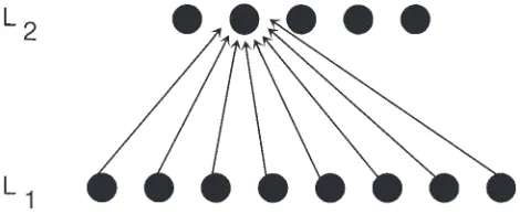
4.1. A learning module

As a first step in building a localist system, I will identify a very simple module capable of unsupervised, self-organized learning of individual patterns and/or pattern classes. This work draws heavily on the work of Carpenter and Grossberg and colleagues (e.g., Carpenter & Grossberg 1987a; 1987b; a debt that is happily acknowledged), with a number of simplifications. The module (see Fig. 3) comprises two layers of nodes, L₁and L₂, fully con-nected to each other by modifiable, unidirectional (L₁-to-L₂) con-nections, which, prior to learning, have small, random weights, w_ij. (Throughout the paper, w_ijwill refer to the weight of the connec-tion from the ith node in the originating layer to the jth node in the receiving layer.) For simplicity of exposition, the nodes in the lower layer will be deemed to be binary, that is, to have activations (denoted a_i) either equal to zero or to one. The extension to con-tinuous activations will usually be necessary and is easily achieved. The input to the nodes in the upper layer will simply be sum of the activations at the lower layer weighted by the appropriate con-nection weights. In fact, for illustrative purposes, I shall assume here that this input to a given node is divided by a value equal to the sum of the incoming weights to that node plus a small constant (see, e.g., Marshall 1990) – this is just one of the many so-called “normalization” schemes typically used with such networks. Thus the input, I_j, to an upper-layer node is given by

where ais the small constant. Learning of patterns of activation at the lower layer, L₁, is simply achieved as follows. When a pat-tern of activation is presented atL₁, the inputs, I_j, to nodes in the upper layer, L₂, can be calculated. Any node whose vector of in-coming weights is parallel (i.e., a constant multiple of) the vector of activations at L₁will have input, I_j, equal to _{11 a/}1

(oalliwij). Any L₂node whose vector of incoming weights is orthogonal to the current input vector (that is, nodes for which w_ij50 where a_i5

1) will have zero input. Nodes with weight vectors between these two extremes, whose weight vectors “match” the current activa-tion vector to some nonmaximal extent, will have intermediate val-ues of I_j. Let us suppose that, on presentation of a given L₁ pat-tern, no L₂node achieves an input, I_j, greater than a threshold u. (With uset appropriately, this supposition will hold when no learn-ing has yet been carried out in the L₁-to-L₂connections.) In this case, learning of the current input pattern will proceed. Learning will comprise setting the incoming weights to a single currently “uncommitted” L₂node (i.e., a node with small, random incom-ing weights) to equal the correspondincom-ing activations at L₁– a

pos-Figure 3. A simple two-layer module.

(1)

I a w

w j

i ij

ij

=

(

)

∑

sible mechanism is discussed later. The learning rule might thus be stated

where Jindexes the single L₂node at which learning is being per-formed, lis the learning rate, and, in the case of so-called “fast learning,” the weight values reach their equilibrium values in one learning episode, such that w_iJ5a_i. The L₂node indexed by Jis thereafter labelled as being “committed” to the activation pattern at L₁, and will receive its maximal input on subsequent presenta-tion of that pattern.

The course of learning is largely determined by the setting of the threshold, u. This is closely analogous to the vigilance pa-rameter in the adaptive resonance theory (ART) networks of Car-penter and Grossberg (1987a; 1987b), one version of which (ART2a, Carpenter et al. 1991) is very similar to the network de-scribed here. More particularly, if the threshold is set very high, for example, u 51, then each activation pattern presented will lead to a learning episode involving commitment of a previously uncommitted L₂node, even if the same pattern has already been learned previously. If the threshold is set slightly lower, then only activation patterns sufficiently different from previously pre-sented patterns will provoke learning. Thus novel patterns will come to be represented by a newly assigned L₂node, without in-terfering with any learning that has previously been accomplished. This is a crucial point in the debate between localist and distrib-uted modellers and concerns “catastrophic interference,” a topic to which I shall return in greater depth later.

The value of the threshold, u, need not necessarily remain con-stant over time. This is where the concept of vigilance is useful. At times when the vigilance of a network is low, new patterns will be unlikely to be learned and responses (see below) will be based on previously acquired information. In situations where vigilance, u, is set high, learning of the current L₁pattern is likely to occur. Thus learning can, to some extent, be influenced by the state of vigilance in which the network finds itself at the time of pattern presentation.

In order to make these notions more concrete, it is necessary to describe what constitutes a response for the network described above. On presentation of a pattern of activation atL₁, the inputs to the L₂nodes can be calculated as above. These inputs are then thresholded so that the net input, I_jnet_{, to the upper-layer nodes is} given by

I_jnet_{5max (0,[I}

j2 u]), (3)

so that nodes I_jwith less than uwill receive no net input, and other nodes will receive net input equal to the degree by which I_j ex-ceeds u. Given these net inputs, there are several options as to how we might proceed. One option is to allow the L₂activations to equilibrate via the differential equation

which reaches equilibrium when daj

dt 50, that is, when ajis some function, f,of the net input. A common choice is to assume thatf

is the identity function, so that the activations equal the net inputs. Another option, which will be useful when some sort of decision process is required, is to allow the L₂nodes to compete in some way. This option will be developed in some detail in the next section because it proves to have some very attractive properties. For the moment it is sufficient to note that a competitive process can lead to the selection of one of the L₂nodes. This might be achieved by some winner-takes-allmechanism, by which the L₂

nodes compete for activation until one of them quenches the ac-tivation of its competitors and activates strongly itself. Or it may take the form of a “horse-race,” by which the L₂nodes race, un-der the influence of the bottom-up inputs, I_jnet_{, to reach a}

crite-rion level of activation,x. Either way, in the absence of noise, we will expect the L₂node with the greatest net input, I_jnet_{, to be} se-lected. In the case where theJth L₂node is selected, the pattern at L₁will be deemed to have fallen into the Jth pattern class. (Note that in a high-uregime there may be as many classes as patterns presented.) On presentation of a given input pattern, the selection (in the absence of noise) of a given L₂node indicates that the cur-rent pattern is most similar to the pattern learned by the selected node, and that the similarity is greater than some threshold value. To summarize, in its noncompetitive form, the network will re-spond so that the activations of L₂nodes, in response to a given input (L₁) pattern, will equilibrate to values equal to some func-tion of the degree of similarity between their learned pattern and the input pattern. In its competitive form the network performs a classification of the L₁activation pattern, where the classes cor-respond to the previously learned patterns. This results in sus-tained or super-criterion activation (a_j. x) of the node that has previously learned the activation pattern most similar to that cur-rently presented. In both cases, the network is self-organizingand

unsupervised.“Self-organizing” refers to the fact that the network can proceed autonomously, there being, for instance, no separate phases for learning and for performance. “Unsupervised” is used here to mean that the network does not receive any external “teaching” signal informing it how it should classify the current pattern. As will be seen later, similar networks will be used when supervised learning is required. In the meantime, I shall simply assume that the selection of an L₂node will be sufficient to elicit a response associated with that node (cf. Usher & McClelland 1995).

4.2. A competitive race

In this section I will give details of one way in which competition can be introduced into the simple module described above. Al-though the network itself is simple, I will show that it has some ex-tremely interesting properties relating to choice accuracy and choice reaction-time. I make no claim to be the first to note each of these properties; nonetheless, I believe the power they have in combination has either gone unnoticed or has been widely un-derappreciated.

Competition in the layer L₂is simulated using a standard “leaky integrator” model that describes how several nodes, each driven by its own input signal, activate in the face of decay and competi-tion (i.e., inhibicompeti-tion) from each of the other nodes:

where Ais a decay constant; I_jis the excitatory input to the jth node, which is perturbed by zero-mean Gaussian noise, N₁, with variance s2

1;f1(aj) is a self-excitatory term; C okÞj f2 (ak)

re-presents lateral inhibition from other nodes in L₂; and N₂ repre-sents zero-mean Gaussian noise with variance s2

2. The value of

the noise term, N₁, remains constant over the time course of a single competition since it is intended to represent inaccuracies in “measurement” of I_j. By contrast, the value of N₂varies with each time step, representing moment-by-moment noise in the calculation of the derivative. Such an equation has a long history in neural modelling, featuring strongly in the work of Grossberg from the mid 1960s onwards and later in, for instance, the cas-cade equation of McClelland (1979).

4.2.1. Reaction time. Recently, Usher and McClelland (1995) have used such an equation to model the time-course of percep-tual choice. They show that, in simulating various two-alternative forced choice experiments, the above equation subsumes optimal classical diffusion processes (e.g., Ratcliff 1978) when a response criterion is placed on the difference between the activations, a_j, of two competing nodes. Moreover, they show that near optimal per-formance is exhibited when a response criterion is placed on the

(2)

dw

dt a w

iJ

i iJ

= l( − ),

(4)

da

dt a f I

j

j j

= − + ( net),

(5)

da

dt Aa I N f a C f a N

j

j j j k

k j

= − + + + − +

≠

∑

absolute value of the activations (as opposed to the difference be-tween them) in cases where, as here, mutual inhibition is assumed. The latter case is easily extensible to multiway choices. This lat-eral inhibitory model therefore simulates the process by which multiple nodes, those in L₂, can activate in response to noisy, bot-tom-up, excitatory signals, Inet_{, and compete until one of the} nodes reaches a response criterion based on its activation alone. Usher and McClelland (1995) have thus shown that a localist model can give a good account of the time course of multiway choices.

4.2.2. Accuracy and the Luce choice rule.Another interesting feature of the lateral inhibitory equation concerns the accuracy with which it is able to select the appropriate node (preferably that with the largest bottom-up input, I_j) in the presence of input noise,

N₁, and fast-varying noise, N₂. Simulations show that in the case where the variances of the two noise terms are approximately equal, the effects of the input noise, N₁, dominate – this is simply because the leaky integrator tends to act to filter out the effects of the fast-varying noise, N₂. As a result, the competitive process tends to “select” that node which receives the maximal noisy in-put, (I_jnet_1N

1). This process, by which a node is chosen by adding zero-mean Gaussian noise to its input term and picking the node with the largest resultant input, is known as a Thurstonian process (Thurstone 1927, Case V). Implementing a Thurstonian process with a lateral-inhibitory network of leaky integrators, as above, rather than by simple computation, allows the dynamics as well as the accuracy of the decision process to be simulated.

The fact that the competitive process is equivalent to a classical Thurstonian (noisy-pick-the-biggest) process performed on the inputs, I_j, is extremely useful because it allows us to make a link with the Luce choice rule (Luce 1959), ubiquitous in models of choice behaviour. This rule states that, given a stimulus indexed by i,a set of possible responses indexed by j,and some set of sim-ilarities, hij, between the stimulus and those stimuli associated with each member of the response set, then the probability of choosing any particular response, J,when presented with a stim-ulus, i,is

Naturally this ensures that the probabilities add up to 1 across the whole response set. Shepard (1958; 1987) has proposed a law of generalization which states, in this context, that the similarities of two stimuli are an exponential function of the distance between those two stimuli in a multidimensional space. (The character of the multidimensional space that the stimuli inhabit can be re-vealed by multidimensional scaling applied to the stimulus-re-sponse confusion matrices.) Thus hij5e2dij, where

where the distance is measured in M-dimensional space, i_m rep-resents the coordinate of stimulus ialong the mth dimension, and

c_mrepresents a scaling parameter for distances measured along dimension m.The scaling parameters simply weigh the contribu-tions of different dimensions to the overall distance measure, much as one might weigh various factors such as reliability and colour when choosing a new car. Equation 7 is known as the Minkowski power model formula and d_ijreduces to the “city-block” distance for r51 and the Euclidean distance for r 52, these two measures being those most commonly used.

So how does the Luce choice rule acting over exponentiated distances relate to the Thurstonian (noisy choice) process de-scribed above? The illustration is easiest to perform for the case of two-alternative choice, and is the same as that found in Mc-Clelland (1991). Suppose we have a categorization experiment in

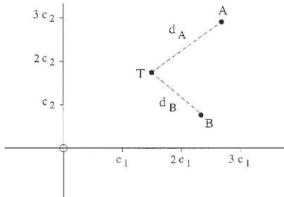
which a subject sees one exemplar of a category A and one exem-plar of a category B. We then present a test exemexem-plar, T,and ask the subject to decide whether it should be categorized as being from category A or category B. Suppose further that each of the three exemplars can be represented by a point in an appropriate multidimensional space such that the test exemplar lies at a dis-tance dAfrom the A exemplar and dBfrom the B exemplar. This situation is illustrated for a two-dimensional space in Figure 4. Note that coordinates on any given dimension are given in terms of the relevant scaling parameters, with the increase of a given scaling parameter resulting in an increase in magnitude of dis-tances measured along that dimension and contributing to the overall distance measures dAand dB. (It is for this reason that an increase of scaling parameter along a given dimension is often de-scribed as a stretching of space along that dimension.) The Luce choice rule with exponential generalization implies that the prob-ability of placing the test exemplar in category A is

dividing top and bottom by e2dA_gives

which equals 0.5 when dA5dB. This function is called the logis-tic function, and it is extremely similar to the function describing the (scaled) cumulative area under a normal (i.e., Gaussian) curve. This means that there is a close correspondence between the two following procedures for probabilistically picking one of two re-sponses at distances dAand dBfrom the current stimulus: one can either add Gaussian noise to dAand dBand pick the category corresponding to, in this case, the smallest resulting value (a Thurstonian process); or one can exponentiate the negative dis-tances and pick using the Luce choice rule. The two procedures will not give identical results, but in most experimental situations will be indistinguishable (e.g., Kornbrot 1978; Luce 1959; Nosof-sky 1985; van Santen & Bamber 1981; Yellott 1977). (In fact, if the noise is double exponential rather than Gaussian, the correspon-dence is exact; see Yellott 1977.)

The consequences for localist modelling of this correspon-dence, which extends to multichoice situations, are profound. Two things should be kept in mind. First, a point in multidimensional space can be represented by a vector of activations across a layer of nodes, say the L1layer of the module discussed earlier, and/or by a vector of weights, perhaps those weights connecting the set of L1nodes to a given L2node. Second, taking two nodes with activations dAand dB, adding zero-mean Gaussian noise, and pick-(6)

p J i iJ

ik

( | )= .

∑

h h all k

(7)

dij cm im jm r m

M r

= −

  

    =

∑

|

|

/ , 1

1

Figure 4. Locations of exemplars A and B and test pattern T in a two-dimensional space. The distances d_Aand d_Bare Euclidean distances, and coordinates on each dimension are given in terms of scaling parameters, c_i.

(8)

p e

e e

d

d d

A

A B

(test is an A)=

+ −

− − ;

(9)

p

edA dB

(test is an A)=

+ −

1 1

ing the node with the smallest resulting activation is equivalent, in terms of the node chosen, to taking two nodes with activations (k2d_A) and (k2d_B) (where kis a constant), adding the same zero-mean Gaussian noise and this time picking the node with the largest activation. Consequently, suppose that we have two L₂

nodes, such that each has a vector of incoming weights corre-sponding to the multidimensional vector representing one of the training patterns, one node representing pattern A,the other node representing pattern B.Further, suppose that on presentation of the pattern of activations corresponding to the test pattern, T,at layer L₁, the inputs, I_j, to the two nodes are equal to (k2d_A) and (k2d_B), respectively (this is easily achieved). Under these cir-cumstances, a Thurstonian process, like that described above, which noisily picks the L₂node with the biggest input will give a pattern of probabilities of classifying the test pattern either as an

Aor, alternatively, as a B,which is in close correspondence to the pattern of probabilities that would be obtained by application of the Luce choice rule to the exponentiated distances, e2dij (Equa-tion 9).

4.2.3. Relation to models of categorization.This correspondence means that mathematical models, such as Nosofsky’s generalized context model (Nosofsky 1986), can be condensed, doing away with the stage in which distances are exponentiated, and the stage in which these exponentiated values are manipulated, in the Luce formulation, to produce probabilities (a stage for which, to my knowledge, no simple “neural” mechanism has been suggested1_), leaving a basic Thurstonian noisy choice process, like that above, acting on (a constant minus) the distances themselves. Since the generalized context model (Nosofsky 1986) is, under certain con-ditions, mathematically equivalent to the models of Estes (1986), Medin and Schaffer (1978), Oden and Massaro (1978), Fried and Holyoak (1984), and others (see Nosofsky 1990), all these models can, under those conditions, similarly be approximated to a close degree by the simple localist connectionist model described here. A generalized exemplar model is obtained under high-u(i.e., high threshold or high vigilance) conditions, when all training patterns are stored as weight vectors abutting a distinct L₂node (one per node).

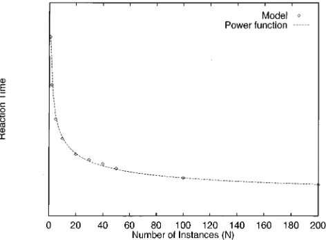
4.2.4. Effects of multiple instances.We can now raise the ques-tion of what happens when, in the simple two-choice categoriza-tion experiment discussed above, the subject sees multiple pre-sentations of each of the example stimuli before classifying the test stimulus. To avoid any ambiguity I will describe the two training stimuli as “exemplars” and each presentation of a given stimulus as an “instance” of the relevant exemplar. For example, in a given experiment a subject might see ten instances of a single category A exemplar and ten instances of a single category B exemplar. Let us now assume that a high-uclassification network assigns a dis-tinct L₂node to each of the ten instances of the category A exem-plar and to each of the ten instances of the category B exemexem-plar. There will thus be twenty nodes racing to classify any given test stimulus. For simplicity, we can assume that the learned, bottom-up weight vectors to L₂nodes representing instances of the same exemplar are identical. On presentation of the test stimulus, which lies at distance d_A(in multidimensional space) from instances of the category A exemplar and distance d_Bfrom instances of the cat-egory B exemplar, the inputs to the L₂nodes representing cate-gory A instances will be (k2d_A) 1N_1j, where N₁is, as before, the input-noise term and the subscript j(0 #j,10) indicates that the zero-mean Gaussian noise term will have a different value for each of the ten nodes representing different instances. The L₂

nodes representing instances of the category B exemplar will like-wise have inputs equal to (k2d_B) 1N_1j, for 10 #j,20. So what is the effect on performance of adding these extra instances of each exemplar? The competitive network will once again select the node with the largest noisy input. It turns out that, as more and more instances of each exemplar are added, two things happen. First, the noisy-pick-the-biggest process becomes an increasingly

better approximation to the Luce formulation, until for an as-ymptotically large number of instances the correspondence is ex-act. Second, performance (as measured by the probability of pick-ing the category whose exemplar falls closest to the test stimulus) improves, a change that is equivalent to stretching the multidi-mensional space in the Luce formulation by increasing by a com-mon multiplier the values of all the scaling parameters, c_m, in the distance calculation given in Equation 7. For the mathematically inclined, I note that both these effects come about owing to the fact that the maximum value out of Nsamples from a Gaussian dis-tribution is itself cumulatively distributed as a double exponential, exp(2e2ax_{), where ais a constant. The distribution of differences} between two values drawn from the corresponding density func-tion is a logistic funcfunc-tion, comparable with that implicit in the Luce choice rule (for further details see, e.g., Yellott 1977; Page & Nimmo-Smith, in preparation).

To summarize, for single instances of each exemplar in a cate-gorization experiment, performance of the Thurstonian process is a good enough approximation to that produced by the Luce choice rule such that the two are difficult to distinguish by experiment. As more instances of the training exemplars are added to the net-work, the Thurstonian process makes a rapid approach toward an asymptotic performance that is precisely equivalent to that pro-duced by application of the Luce choice rule to a multidimen-sional space that has been uniformly “stretched” (by increasing by a common multiplier the values of all the scaling parameters, c_m, in Equation 7) relative to that space (i.e., the set of scaling pa-rameters) that might have been inferred from the application of the same choice rule to the pattern of responses found after only a single instance of each exemplar had been presented. It should be noted that putting multiple noiseless instances into the Luce choice rule will not produce an improvement in performance rel-ative to that choice rule applied to single instances – in mathe-matical terminology, the Luce choice rule is insensitive to uniform expansion of the set (Yellott 1977).

Simulations using the Luce formulation (e.g., Nosofsky 1987) have typically used uniform multiplicative increases in the values of the dimensional scaling parameters (the c_min Equation 7) to account for performance improvement over training blocks. The Thurstonian process described here, therefore, has the potential advantage that this progressive space-stretching is a natural fea-ture of the model as more instances are learned. Of course, until the model has been formally fitted to experimental data, the sug-gestion of such an advantage must remain tentative – indeed early simulations of data from Nosofsky (1987) suggest that some para-metric stretching of stimulus space is still required to maintain the excellent model-to-data fits that Nosofsky achieved (Page & Nimmo-Smith, in preparation). Nonetheless, the present Thurs-tonian analysis potentially unites a good deal of data, as well as rais-ing a fundamental question regardrais-ing Shepard’s “universal law of generalization.” Could it be that the widespread success encoun-tered when a linear response rule (Luce) is applied to representa-tions with exponential generalization gradients in multidimen-sional stimulus space is really a consequence of a Thurstonian decision process acting on an exemplar model, in which each of the exemplars actually responds with a linear generalization gra-dient? It is impossible in principle to choose experimentally be-tween these two characterizations for experiments containing a reasonable number of instances of each exemplar. The Thurston-ian (noisy-pick-the-biggest) approach has the advantage that its “neural” implementation is, it appears, almost embarrassingly simple.