Faster Homomorphic Linear Transformations in HElib

(1)

Faster Homomorphic Linear Transformations in

HElib

?

Shai Halevi1 _{and Victor Shoup}1,2

1

IBM Research 2 _{New York University}

June 1, 2018

Abstract. HElibis a software library that implements homomorphic encryption (HE), with a focus on effective use of “packed” ciphertexts. An important operation is applying a known linear map to a vector of encrypted data. In this paper, we describe several algorithmic improvements that significantly speed up this operation: in our experiments, our new algorithms are 30–75 times faster than those previously implemented inHElibfor typical parameters. One application than can benefit from faster linear transformations is bootstrapping (in particular, “thin bootstrapping” as described in [Chen and Han, Eurocrypt 2018]). In some settings, our new algorithms for linear transformations result in a 6×

speedup for the entire thin bootstrapping operation. Our techniques also reduce the size of the large public evaluation key, often using 33%-50% less space than the previous HElib implementation. We also implemented a new tradeoff that enables a drastic reduction in size, resulting in a 25×factor or more for some parameters, paying only a penalty of a 2-4×times slowdown in running time (and giving up some parallelization opportunities).

Keywords.Homomorphic encryption, Implementation, Linear transformations

?_{Supported by the Defense Advanced Research Projects Agency (DARPA) and Army Research Office(ARO) under}

(2)

Homomorphic encryption (HE) [13, 5] enables performing arithmetic operations on encrypted data even without knowing the secret key. All contemporary HE schemes roughly follow the outline of Gentry’s first candidate, where fresh ciphertexts are “noisy” to ensure security. This noise grows with every operation, until it becomes so large so as to cause decryption errors. This results in a “somewhat homomorphic” encryption scheme (SWHE) that can only evaluate low-depth cir-cuits, such a scheme can be converted to a “fully homomorphic” encryption scheme (FHE) using bootstrapping. The most asymptotically efficient SWHE schemes are based on the hardness of ring-LWE. Most of these scheme use Rp = Z[X]/(F(X), p) as their native plaintext space, with F a

cyclotomic polynomial and pan integer (usually a prime or prime power).

Smart and Vercauteren observed [15] that (for a prime p) an element in this native plaintext space can be used to encode (via Chinese Remaindering) a vector of values from a finite field

Fpd, for some integer d that depends on F and p, and that operations on elements in Rp induce

the corresponding entry-wise operation on the encoded vectors. This technique of encoding many plaintext elements from Fpd in a single R_p element, which is then encrypted and manipulated

homomorphically, is called “ciphertext packing”, and the entries in the vector are called “plaintext slots.” Gentry, Halevi, and Smart showed in [6] how to use special automorphisms on Rp (which were used for different purposes in [10] and [2]) to enable data movement between the slots.

HElib[9, 7, 8] is an open-sourceC++ library that implements the ring variant of the scheme due to Brakerski-Gentry-Vaikuntanathan [2], focusing on effective use of ciphertext packing. It includes an implementation of the BGV scheme itself with all its basic homomorphic operations, as well as higher-level procedures for data-movement, simple linear algebra, bootstrapping, etc. One can think of the lower levels of HElibas providing a “hardware platform”, defining a set of operations that can be applied homomorphically. These operations include entry-wise addition and multiplication operations on the vector of plaintext values, as well as data movement, making this “platform” a SIMD environment.

Our Results. In this work, we improve performance of core linear algebra algorithms in HElibthat apply publicly known linear transformations to encrypted vectors. These improvements are now integrated into HElib. For typical, realistic parameter settings, our new algorithms can run 30-75 times faster than those in the previous implementation of HElib, where the exact speedup depends on myriad details.3 Our implementation also exploits multiple cores, when available, to get even further speedups.

Our techniques also reduce the size of the large public evaluation key. In the old HElib imple-mentation, the evaluation key typically consists of a large number of large “key switching matrices”: Each of these “matrices” can take 1-4MB of space, and the implementation uses close to a hundred of them. Our new implementation reduces the number of key-switching matrices by 33–50% in some parameter settings (that arise fairly often in practice), while at the same time improves the running time. Moreover, a new tradeoff that we implemented enables a drastic reduction in the number of matrices (sometimes as few as four or six matrices overall), for a small price of only 2-4× in performance. This space efficient variation, however, is inherently sequential, as opposed to our other procedure than can be easily parallelized.

3

(4)

Applications. Linear transformations of encrypted vectors is a manifestly fundamental operation with many applications. For one example,HElibitself makes critical use of such transformations in its bootstrapping logic. As reported in [8], the bootstrapping routine can typically spend 25–40% of its time performing such transformations. In addition, a new “thin bootstrapping” technique, due to Chen and Han [4], is useful to bootstrap encrypted vectors whose entries are in the base field, rather than an extension field. In practice, this is an important special case of bootstrapping, and our faster algorithms for linear transformations play an even more significant role here. Our timing results in Section 9 show that for large vectors, these faster algorithms are essential to make “thin bootstrapping” practical.

As another example, consider a private information retrieval protocol in which a client selects one value from a database of values held by a server, while hiding from the server which value was accessed. Using HE, one way to do this is for the server to encode each value as a column vector. The collection of all such values held by the server is thus encoded as a matrix M, where each column in M corresponds to one value. To access the ith value, the client can send to the server an encrypted unit vector v with 1 in the ith entry (or some other encrypted information from which the server can homomorphically compute such an encrypted unit vector). The server then homomorphically computes M×v, which is an encryption of the selected column ofM. The server sends the result to the client, who can decrypt it and recover the selected value.

Techniques. In the linear transformation algorithms previously implemented in HElib, the bulk of the time is spent moving data among the slots in the encrypted vector. As mentioned above, this is accomplished by using special automorphisms. The main cost of applying such an automorphism to a ciphertext is actually that of “key switching”: after applying the automorphism to each ring element in the ciphertext (which is actually a very cheap operation), we end up with an encryption relative to the “wrong” secret key; we can recover a ciphertext relative to the “right” secret key by using data in the public key specific to this particular automorphism — a so-called “key switching matrix.”

The main goals in improving performance are therefore to reduce the number of automorphisms, and to reduce the cost of each automorphism.

– To reduce the number of automorphisms, we introduce a “baby-step/giant-step” strategy for computing all of the required automorphisms. This strategy generalizes a similar idea that was used in [8] in the context of bootstrapping. This strategy by itself speeds up the computation by a factor of 15–20 in typical settings. See Section 4.1.

– We further reduce the number of automorphisms by refactoring a number of computations, more aggressively exploiting the algebraic properties of the automorphisms that we use. See Section 4.4.

– To reduce the cost of each automorphism, we introduce a new technique for “hoisting” the expensive parts of these operations out of the main loop.4Our main observation is that applying many automorphisms to the same ciphertext v can be done faster than applying each one separately. Instead we can perform an expensive pre-computation that depends only on v (but not the automorphisms themselves), and this pre-computation makes each automorphism much cheaper (typically, 6–8 times faster). See sections 4.2 and 5.

4_{“Hoisting” is a term used in compiler optimization to describe the action of “hoisting” a computation out of a}

(5)

– Recall that key switching matrices are a part of the public key, we note that they consume quite a lot of space (typically several megabytes per matrix), so keeping their numbers down is desirable. In the previous implementation of HElib, there can easily be several hundred such matrices in the public key. We introduce a new technique that reduces the number of key-switching matrices by 33–50% in some parameter settings (that arise fairly often in practice), while at the same time improves the running time of our algorithms. See Section 4.3.

– We introduce yet another technique that drastically reduces the number of key-switching ma-trices to a very small number (less than 10), but comes at a cost in running time (typically 2–4 times more slowly as our fastest algorithms), and cannot be parallelized.5 Achieving this reduction in key-switching storage without too much degradation in running time requires some new algorithmic ideas. See Section 4.5.

Outline. The rest of the paper is organized as follows.

– In Section 2, we introduce notation and terminology, and review the basics of the BGV cryp-tosystem, including ciphertext packing and automorphisms.

– In Section 3, we review the basic ideas underlying the previous algorithms in HElibfor apply-ing linear transformations homomorphically. We focus on restricted linear transformations, the “one-dimensional” transformationsMatMul1Dand BlockMatMul1D. It turns out that consider-ing these restricted transformations is sufficient: they can be used directly in applications such as bootstrapping, and can be easily be used to implement more general linear transformations. – In Section 4, we give a more detailed overview of our new techniques.

– In Section 5, we give more of the details of our new hoisting technique.

– In Section 6, we present all of our new algorithms for MatMul1DandBlockMatMul1Din detail. – In Section 7, we describe how to use algorithms for MatMul1D and BlockMatMul1D for more

general linear transformations.

– In Section 8, we review the bootstrapping procedure from [8], and discuss how those techniques can be adpated to the “thin bootstrapping” technique of Chen and Han [4].

– In Section 9, we report on the performance of the implementation of our new algorithms (and their application to bootstrapping).

2 Notations and Background

For a positive modulus q ∈ _Z_>₀, we identify the ring Zq with its representation as integers in [−q/2, q/2) (except for q = 2 where we use {0,1}). For integer z, we denote by [z]q the reduction of z modulo q into the same interval. This notation extends to vectors and matrices coordinate-wise, and to elements of other algebraic groups/rings/fields by considering their coefficients in some convenient basis (e.g., the coefficient of polynomials in the power basis when talking aboutZ[X]).

The norm of a ring element kakis defined as the norm of its coefficient vector in that basis.6

5

While the “top level” operations in our linear transformations are inherently sequential when using this technique, lower-level routines inHElibwill still exploit multiple cores, if available. Such low-level parallelism are usually less effective, however.

6

(6)

2.1 The BGV Cryptosystem

The BGV ring-LWE-based scheme [3] is defined over a ring R def= Z[X]/(Φm(X)), where Φm(X)

is the mth cyclotomic polynomial. For an arbitrary integer modulus N (not necessarily prime) we denote the ring RN def= R/N R.

As implemented inHElib, the native plaintext space of the BGV cryptosystem isRpr for a prime

power pr_{. The scheme is parametrized by a sequence of decreasing moduli} _q

LqL−1 · · · q0,

and an “ith level ciphertext” in the scheme is a vector v ∈ R2_q_i. Secret keys are elements s ∈ R with “small” coefficients (chosen in{0,±1} inHElib), and we view sas the second element of the 2-vector sk = (1, s) ∈ R2_{. A level-i} _ciphertext _v _{= (p}

0, p1) encrypts a plaintext element α ∈ Rpr

with respect to sk = (1, s) if [hsk, vi]q_i = [p0+s·p1]qi =α+p

r_·_(in _{R) for some “small” error} term, kk qi/pr.

The error term grows with homomorphic operations of the cryptosystem, and switching from qi+1 toqi is used to decrease the error term roughly by the ratio qi+1/qi. Once we have a level-0

ciphertextv, we can no longer use that technique to reduce the noise. To enable further computation, we need to use Gentry’s bootstrapping technique [5]. InHElib, eachqiis a product of small (machine-word sized) primes.

2.2 Encoding Vectors in Plaintext Slots

As observed by Smart and Vercauteren [15], an element of the native plaintext space α ∈ Rpr

can be viewed as encoding a vector of “plaintext slots” containing elements from some smaller ring extension of Zpr via Chinese remaindering. In this way, a single arithmetic operation on α

corresponds to the same operation applied component-wise to all the slots.

Specifically, suppose the factorization of Φm(X) modulo pr is Φm(X) ≡ F1(X)· · ·F`(X) (modpr_{), where each} _F

i has the same degree d, which is equal to the order of p modulo m, so that ` =φ(m)/d. (This factorization can be obtained by factoring Φm(X) modulo p, followed by Hensel lifting.) Then we have the isomorphismRpr ∼=L`

i=1(Z[X]/(pr, Fi(X)).

Let us now denote E def= Z[X]/(pr, F1(X)), and let ζ be the residue class of X in E, which is

a principal mth root of unity, so that E =Z/(pr)[ζ]. The rings Z[X]/(pr, Fi(X)) fori = 1, . . . , `

are all isomorphic to E, and their direct product is isomorphic to Rpr, so we get an isomorphism

betweenRpr andE`.HElibmakes extensive use of this isomorphism, using it to encode an`-vector

of elements in E as an element of the native plaintext space Rpr. Addition and multiplication of

ciphertexts act on all`slots of the corresponding plaintext in parallel.

2.3 Hypercube structure and one-dimensional rotations

Beyond addition and multiplications, we can also manipulate elements in Rpr using a set of

auto-morphisms on Rpr of the form

θt:Rpr −→R_pr, a(X)7−→a(Xt) (mod (pr, Φ_m(X))).

fort∈Z∗m. Since eachθt is an automorphism, it distributes over addition and multiplication, i.e., θt(α+β) =θt(α) +θt(β) and θt(αβ) =θt(α)θt(β). Also, these automorphisms commute with one another, i.e., θtθt0 =θ_tt0 =θ_t0θ_t. Moreover, for any integeri, we have θi_t=θ_ti.

(7)

ciphertext in HElibconsists of two “parts,” each an element of Rq for some q. Applying the same automorphism (defined in Rq) to the two parts, we get a ciphertext with respect to a different secret key. In order to do anything more with this ciphertext, we usually have to convert it back to a ciphertext with respect to the original secret key. In order to do this, the public-key must contain data specific to the automorphismθt, called a “key switching matrix”.7We will discuss this key-switching operation in more detail below in Section 5.

As discussed in [6], these automorphisms induce a hypercube structure on the plaintext slots, that depends on the structure of the group Z∗m/hpi. Specifically, HElib keeps a hypercube basis g1, . . . , gn ∈ Z∗m with orders D1, . . . , Dn ∈ Z>0, and then defines the set of representatives for Z∗m/hpias

{ge1 1 · · ·g

en

n : 0≤es< Ds, s= 1, . . . , n}.

More precisely, Ds is the order of gs in Z∗m/hp, g1, . . . , gs−1i. Thus, the slots are in one-to-one

correspondence with tuples (e1, . . . , en) with 0≤es< Ds. This induces ann-dimensional hypercube

structure on the plaintext space. If we fixe1, . . . , es−1, es+1, . . . , en, and letesrange over 0, . . . , Ds− 1, we get a set ofDs slots, which we refer to as ahypercolumn in dimension s(and there are`/Ds such hypercolumns).

Using automorphisms, we can efficiently perform rotations in any dimension; a rotation by

i in dimension s maps a slot corresponding to (e1, . . . , es, . . . , en) to the slot corresponding to (e1, . . . , es+imodDs, . . . , en). In other words, it rotates each hypercolumn in dimension s by i.

We denote by ρs the rotation-by-1 operation in dimension s. Observe that ρis is the rotation-by-i operation in dimension s.

We can implement ρi_s by applying either one or two of the automorphisms {θt}t∈Z∗m defined

above. If the order of gs inZ∗m is Ds, then we get by with just a single automorphism, since

ρi_s(α) =θgi

s(α). (1)

In this case, we call sa “good dimension”.

If the order of gsinZ∗m is different fromDs, then we call sa “bad dimension”, and we need to implement this rotation using two automorphisms. Specifically, we use a constant “0-1 mask value” µ that selects some slots and zeros-out the others, and use the two automorphisms ψ def= θ_gi

s and

ψ∗ def= θ_gi−D

s . Then we have

ρi_s(α) =ψ(µ·α) +ψ∗((1−µ)·α). (2)

The idea is roughly as follows. Even though ψ does not act as a rotation by i in dimension s, it does act as the desired rotation if we restrict it to inputs with zeros in each slot whose coordinate in dimensionsis at leastD−i. Similarly,ψ∗ acts as the desired rotation if we restrict it to inputs with zeros in each slot whose coordinate in dimension s is less than D−i. This tells us that µ should have a 1 in all slots whose coordinate in dimensionsis less thanD−i, and a 0 in all other slots. Note also that

ρi_s(α) =µ0·ψ(α) + (1−µ0)·ψ∗(α), (3)

whereµ0 =ψ(µ) is a mask with a 1 is all slots whose coordinate in dimensionsis at least i, and a 0 in all other slots. This formulation will be convenient in some of the algorithms we present.

7

(8)

2.4 Frobenius and linearized polynomials

We define the automorphism σ def= θp, which is the Frobenius map on Rpr (where θ_p is one of the

automorphisms defined in Section 2.3). It acts on each slot independently as the Frobenius map σE on E, which sends ζ to ζp and leaves elements of Zpr fixed. (When r = 1, σ is the same as

thepth power map on E.) For anyZpr-linear transformation onE, denotedM, there exist unique

constantsλ0, . . . , λd−1∈Esuch thatM(η) =Pdj−=01λjσ

j

E(η) for allη∈E. Whenr= 1, this follows from the general theory of linearized polynomials (see, e.g., Theorem 10.4.4 on p. 237 of [14]), but the same results are easily seen to hold for r >1 as well. These constants are readily computable by solving a system of equations modpr.

Using linearized polynomials, we may effectively apply a fixed linear map to each slot of a plain-text elementα∈Rpr (either the same or different maps in each slot) by computingPd_j₌₀−1κjσj(α),

where theκj’s areRpr-constants obtained by embedding appropriate E-constants in the slots.

2.5 Key switching strategies

The total number of automorphisms is φ(m), which is typically many thousands, so it is not very practical to store all possible key switching matrices in the public key: each such matrix typically occupies a few megabytes of storage, and storing all of them will consume hundreds of gigabytes. Therefore, we consider strategies that trade off space for time with respect to key switching matrices. For almost all applications, we only need the key switching matrices for one-dimensional rota-tions in each dimension, as well as for the Frobenius map (and its powers). For a fixed dimension

s= 1, . . . , n of size Ddef= Ds with generator g

def

= gs, consider the automorphism θ

def

= θgs. In the

original implementation of HElib, one of two key switching strategies for dimensionsare used.

Full: We store key switching matrices for θi for i = 0, . . . , D−1. If s is a “bad dimension”, we additionally store key switching matrices for θ−i fori= 1, . . . , D−1.

Baby-step/giant-step: We store key switching matrices for θj with j = 1, . . . , g −1, where gdef= d√De(the “baby steps”), as well as for θgk withk= 1, . . . , h−1, where hdef= dD/ge (the “giant steps”). If sis a “bad dimension”, we additionally store key switching matrices for θ−gk with k= 1, . . . , h(negative “giant steps”).

Using the full strategy, any rotation in dimensionscan be implemented using a single automor-phism and key switching ifsis a good dimension, and using two automorphisms and key switchings ifsis a bad dimension.

Using the baby-step/giant-step strategy, any rotation in dimensionscan be implemented using at most two automorphisms and key switchings if s is a good dimension, and using at most four automorphisms and key switchings ifs is a bad dimension. The idea is that to compute θi(v), for a given i = 0, . . . , D−1, we can write i = j+gk, so that to compute θi(v), we first compute w =θgk(v), which takes one automorphism and a key switching, and then compute θj(w), which takes another automorphism and key switching.

These two strategies give us a time/space trade-off: although it slows down the computation time by a factor of two, the baby-step/giant-step strategy requires space for just O(√D) key switching matrices, rather than the O(D) key switching matrices required by the full strategy.

(9)

automorphisms. Indeed, it is convenient to think of the powers of the Frobenius map as defining an additional (effectively “good”) dimension.

The default behavior of HElib is to use the full key-switching strategy for “small” dimensions (of size at most 50), and the baby-step/giant-step strategy for larger dimensions.

3 Matrix multiplication — basic ideas

In [7], it is observed that we can multiply a matrix M ∈ E`×` by a column vector v ∈ E`×1 by computing

M v=M0v0+· · ·+M`−1v`−1, (4)

where each vi is the vector obtained by rotating the entries of v by i positions, and each Mi is a diagonal matrix containing one diagonal ofM.

3.1 MatMul1D: one-dimensional E-linear transformations

In many applications, such as the recryption procedure in [8], instead of a general E-linear trans-formation on Rpr, we only need to work with a one-dimensionalE-linear transformation that acts

independently on the individual hypercolumns of a single dimensions= 1, . . . , n. We can adapt the diagonal decomposition of Eqn. (4) to this setting using appropriate rotation maps on the slots of Rpr. Letρdef= ρ_s be the rotation-by-1 map in dimensions, and letDdef= D_sbe the size of dimension

s. IfT is a one-dimensional E-linear transformation onRpr, then for everyv∈Rpr, we have

T(v) = D−1 X

i=0

κi·ρi(v), (5)

where theκi’s are constants inRpr determined byT, obtained by embedding appropriate constants

inE in each slot. Eqn. (5) translates directly into a simple homomorphic evaluation algorithm, just by applying the same operations to a ciphertext encryptingv. In a straightforward implementation, in a good dimension, the computational cost is aboutDautomorphisms andDconstant-ciphertext multiplications, and the noise cost is a single constant-ciphertext multiplication. In bad dimensions, all of these costs would essentially double. In practice, if the constants have been pre-computed, the computation cost of the constant-ciphertext multiplications is negligible compared to that of the automorphisms.

One of our main goals in this paper is to dramatically improve upon the computational cost for performing such aMatMul1D operation.

3.2 BlockMatMul1D: one-dimensional Zpr-linear transformations

In some applications (again, including the recryption procedure in [8]), instead of applying an E-linear transformation, we need to apply a Zpr-linear map. Again, we focus on one-dimensional Zpr-linear maps that act independently on the hypercolumns of a single dimension.

(10)

be encoded using linearized polynomials, as in Section 2.4. Therefore, if T is a one-dimensional

Zpr-linear transformation on R_pr, then for every v∈R_pr, we have

T(v) = D−1

X

i=0

d−1 X

j=0

κi,j·σj ρi(v), (6)

where theκi,j’s are constants in Rpr determined byT.

A naive homomorphic implementation of the formula from Eqn. (6) takes O(dD) automor-phisms, but as shown in [8], this can be reduced to O(d+D) automorphisms. In this paper, we will also present significant improvements to the BlockMatMul1D algorithm in [8], although they are not as dramatic as our improvements to the MatMul1Dalgorithm.

4 Overview of algorithmic improvements

4.1 Baby-step/giant-step multiplication

As already mentioned, [8] introduces a technique that reduces the number of automorphisms needed

to implementBlockMatMul1Din dimensionsfromO(dD) toO(d+D), whereDdef= Dsis the size of the dimension, anddis the order ofpmodm. A very similar idea, essentially a baby-step/giant-step technique, can be used to reduce the number of automorphisms needed to implementMatMul1Din dimensionsfrom O(D) to O(√D). See Section 6 for details.

This technique is distinct from the baby-step/giant-step key switching strategy discussed above in Section 2.5. However, for best results, the two techniques should be combined in a way that harmonizes the baby-step/giant-step thresholds.

4.2 Hoisting

As we have seen, in many situations, we want to compute ψ(v) for a fixed ciphertext v and many automorphisms ψ. Assuming we have key switching matrices for each automorphism ψ, the dom-inant cost of computing all of these values is that of performing one key-switching operation for each ψ. Our “hoisting” technique is a method that refactors the computation, performing a pre-computation that only depends onv, and whose computational cost is roughly equivalent to a single key-switching operation. After performing this pre-computation, computing ψ(v) for any individ-ualψis much faster than a single key-switching operation (typically, around 6–8 times faster). We describe this idea in more detail below in Section 5.

4.3 Better key switching strategies in bad dimensions

(11)

cuts the number of key-switching matrices in half without a significant increase in running time. Moreover, this key-switching strategy aligns well with the strategy discussed below for decoupling rotations and automorphisms in bad dimensions.

Similarly, for the baby-step/giant-step key-switching strategy in a bad dimension, we just store a key-switching matrix for θ−D_{, rather than for all the negative “giant steps”. This cuts down the} number of key-switching matrices by a third. Moreover, the number of key switchings we need to perform per rotation is only 3 (instead of 4).

4.4 Decoupling rotations and automorphisms in bad dimensions

Recall that by Eqn. (3), a rotation by i on a ciphertext v in a given bad dimension can be im-plemented as µθi(v) + (1−µ)θi−D(v), where µ is a “mask” (a constant with a 0 or 1 encoded in each slot). It turns out that in our matrix-vector computations, it is best to work directly with this implementation, and algebraically refactor the computation to improve both running time and noise. This refactoring exploits the fact that θis an automorphism. See Section 6 for details.

4.5 A Horner-like rule with application to a minimal key-switching strategy

We introduce a new key-switching strategy that reduces the storage requirements even further, to just 1, 2, or 3 key-switching matrices per dimension. This, combined with a simple algorithmic idea, allow us to implement a variant of the baby-step/giant-step multiplication strategy that does not run too much more slowly than when using the full or baby-step/giant-step key-switching strategy. To do this, we observe that if we need to compute Ph−1

i=0 ψi(vi), where ψ is some automorphism and thevi’s are ciphertexts, we can do this using Horner’s rule, provided we have a key-switching matrix just for ψ. Specifically, we can compute

h−1 X

i=0

ψi(vi) =ψ · · ·ψ ψ(vh−1) +vh−2

+· · ·

+v0.

That is, we set wh−1 ← vh−1, then wi−1 ← ψ(wi) +vh−1 for i = h−1, . . . ,1, and finally we

output w0.

4.6 Exploiting multi-core platforms

With the exception of the minimal key-switching strategy discussed above, all our other algorithms are very amenable to parallelization. We thus implemented them so as to exploit multiple cores, when available.

5 Hoisting

A ciphertext in HElib is a vector v = (p0, p1) ∈R2q, with each “part” p0, p1 represented in a

Dou-bleCRTformat (i.e., both integer and polynomial CRT) [9]. We recall the steps in the computation of eachψ(v), as implemented inHElib.

(12)

Applying an automorphism to aDoubleCRT object is a fast, linear time operation, so this step is cheap. Ifv = (p0, p1) decrypts to α under the secret key sk= (1, s), thenv0 = (p00, p01) decrypts

toψ(α) under the secret keysk0 = (1, ψ(s)). We next have to perform a “relinearization” operation which converts v0 back to a ciphertext that decrypts to ψ(α) under the original secret keysk. This operation can itself be broken down into two steps:

2. Break into digits: decomposep0₁ into “small” pieces:p0₁=P

kqk0∆k.

Here, the ∆k’s are integer constants, and the pieces q0k are elements of R of small norm. This operation is rather expensive, as it requires conversions between DoubleCRT and coefficient representations of elements inRq.

3. Key switching:compute the ciphertext (p0₀+p00₀, p00₁), where

p00_j =X k

q0_kAjk, (j= 0,1).

Here, the Ajk’s are the “key switching matrices”, namely, pre-computed elements in RQ (for some larger Q) which are stored in the public key. TheAjk’s are stored in DoubleCRT format, so if we have theq_k0 in the sameDoubleCRTformat then this operation is also a fast, linear time operation.

The key observation to our new technique is that we can reverse the order of the first two steps above, without affecting the correctness of the procedure. Namely our new procedure is as follows:

1. Break into digits: decompose the original p1 before applying the automorphism into “small”

pieces: p1=Pkqk∆k.

2. Automorphism: compute p0₀ ← ψ(p0), and qk0 ← ψ(qk) for each qk. Namely, p00 is computed

just as before, but we apply the automorphism to the pieces qk from above rather than to p1

itself.

3. Key switching:compute the ciphertext (p0₀+p00₀, p00₁), where

p00_j =X k

q0_kAjk, (j= 0,1).

This is exactly the same computation as before.

The reasons that this works, is that (i) ψ is an automorphism (so it distributes over addition and multiplication), and (ii) applying ψ does not significantly change the norm of an element (cf. [10]). In a little more detail, correctness of the key-switching step depends only on the following two conditions on theq_k0’s:

(a) P

kqq0∆k=ψ(p1), and

(b) the q0_k’s have low norm.

Condition (a) is satisfied in our new procedure since ψ is an automorphism (which acts as the identity on integers), and so

ψ(p1) =ψ X

k qk∆k

=X k

ψ(qk)∆k =

X

k

(13)

Condition (b) is satisfied since the pieces qk have small norm, and applying ψ to a ring element does not increase its norm significantly.

The new procedure is therefore just as effective as the old one, but now the expensive break-into-digits step can be preformed only once, as a pre-computation that depends only onv, rather than having to perform it for every automorphism ψ. The flip side is that we need to apply ψ to each one of the partsqkinstead of only once to p1. But as we mentioned, this is a cheap operation.

5.1 Interaction with key-switching strategy

If we want to compute ψ(v) for various automorphismsψ, and we have key-switching matrices for all of the ψ’s. then we can apply the above hoisting strategy directly. In some situations, what we want to do is compute θi(v) for i = 0, . . . , D−1, where θ = θgs for some dimension s with

generator gs∈Z∗m, and whereD=Ds is the size of the dimension. If we are employing the baby-step/giant-step strategy for storing key-switching matrices, then we do not have all of the requisite key-switching matrices, so we cannot use the hoisting strategy directly. Instead, what we can do is the following. Since we have key-switching matrices for all of the giant stepsθgj, forj = 1, . . . , h−1, we can use hoisting to compute θgj(v) for all of the giant steps, and for each of these values, we perform the pre-computation (i.e., the break-into-digits step). Then, since we have key-switching matrices for all of the baby steps θk, for k= 1, . . . , g−1, we can compute any value θgj+k(v) as θk( θgj(v) ), using the precomputed data forθgj(v) and the key-switching matrix forθk.

6 Algorithms for one-dimensional linear transformations

In this section, we describe in detail our algorithms for applying one-dimensional linear transfor-mations to a ciphertextv. We fix a dimensions= 1, . . . , n. Recall from Section 2.3 thatρdef= ρs is the rotation-by-1 map in dimensions, and thatDdef= Ds is the size of dimension s.

6.1 Logic for basic MatMul1D

Recall from Section 3.1 that for that MatMul1Dcalculation, we need to compute

w= X i∈[D]

κ(i)ρi(v),

where theκ(i)’s are constants in Rpr that depend on the matrix.

If s is a good dimension, then ρ is realized with a single automorphism, ρ = θ def= θgs where

gs ∈Z∗m is the generator for dimension s. We can easily implement this in a number of ways. For example, we can use the hoisting technique from Section 5 to compute all of the values θi(v) for i∈[D]. Alternatively, if we are using a minimal key-switching strategy (see Section 4.5), then with just a key-switching matrix for θ, we can compute the values θi(v) iteratively, computing θi+1(v) from θi(v) as θ(θi(v)).

6.2 Revised logic for bad dimensions

From Eqn. (3), if sis a bad dimension, then we have

(14)

where µ(i) is a “0-1 mask” and µ0(i) = 1 −µ(i). As discussed in Section 4.4, it is useful to algebraically decouple the rotations and automorphisms in a bad dimension, which we can do as follows:

w= X i∈[D]

κ(i)ρi(v)

= X

i∈[D]

κ(i)µ(i)θi(v) +µ0(i)θi−D(v)

= X

i∈[D]

κ0(i)θi(v) + θ−D

X

i∈[D]

κ00(i)θi(v)

,

where

κ0(i) =µ(i)κ(i) and κ00(i) =θDµ0(i)κ(i)}.

To implement this, we have to compute θi(v) for alli∈[D]. This can be done using the same strategies as were discussed above in a good dimension, using either hoisting or iteration. The only other automorphism we need to compute is one evaluation of θ−D. Note that with our new key-switching strategy (see Section 4.3), we always have available a key-switching matrix for θ−D. If we ignore the cost of pre-computing all the constants in DoubleCRT format, we see that the computational cost is roughly the same in both good and bad dimensions. This is because the time needed to perform all the constant-ciphertext multiplications is very small in comparison to the time needed to perform all the automorphisms. The cost in noise is also about the same, essentially, one constant-ciphertext multiplication.

6.3 Baby-step/giant-step logic

We now present the logic for a new baby-step/giant-step multiplication algorithm. As discussed above in Section 4.1, this idea is very similar to the BlockMatMul1Dimplementation described in [8]. Setg=d√Deand h=dD/ge. We have:

w= X i∈[D]

κ(i)ρi(v)

= X

j∈[g] X

k∈[h]

κ(j+gk)ρj+gk(v)

= X

k∈[h]

ρgk

X

j∈[g]

κ0(j+gk)ρj(v)

,

whereκ0(j+gk) =ρ−gk(κ(j+gk)).

Algorithm 1. In a good dimension, where ρ = θ, we can implement the above logic using the following algorithm.

(15)

2. For each k∈[h], compute

wk =

X

j∈[g]

κ0(j+gk)vj.

3. Compute

w= X k∈[h]

θgk(wk).

Step 1 of the algorithm can be implemented by hoisting, or if we are using a minimal key-switching strategy, by iteration. Also, if we employ the minimal key-key-switching strategy, then Step 3 can be implemented using the Horner-rule idea discussed in Section 4.5 — for this, we just need a key-switching matrix for θg. Otherwise, if we have key switching matrices for all of the ρgk’s, it is somewhat faster to apply all of these automorphisms independently, which is also amenable to parallelization.

6.4 Revised baby-step/giant-step logic for bad dimensions

Setg=d√De and h=dD/ge. Again, using Eqn. (7), and the idea of algebraically decoupling the rotations and automorphisms in a bad dimension, we have:

w= X i∈[D]

κ(i)ρi(v)

= X

i∈[D]

κ(i)µ(i)θi(v) +µ0(i)θi−D(v)

= X

j∈[g] X

k∈[h]

κ(j+gk)

µ(j+gk)θj+gk(v) +µ0(j+gk)θj+gk−D(v)

= X

k∈[h]

θgk

X

j∈[g]

κ0(j+gk)θj(v) +κ00(j+gk)θj−D(v)

,

where

κ0(j+gk) =θ−gk

µ(j+gk)κ(j+gk) and κ00(j+gk) =θ−gk

µ0(j+gk)κ(j+gk) .

Based on this, we derive the following:

Algorithm 2.

1. Compute v0 =θ−D(v).

2. For each j∈[g], compute vj =θj(v) and v0_j =θj(v0) 3. For each k∈[h], compute

wk=

X

j∈[g]

κ0(j+gk)vj+κ00(j+gk)v_j0 .

4. Compute

w= X k∈[h]

(16)

Step 2 of the algorithm can be implemented by hoisting, or if we are using a minimal key-switching strategy, by iteration. Also, if we employ the minimal key-key-switching strategy, then Step 4 can be implemented using Horner’s rule. As before, if we have key switching matrices for all of the ρgk’s, it is somewhat faster to apply all of these automorphisms independently, which is also amenable to parallelization.

Based on experimental data, we find that using the baby-step/giant-step multiplication algo-rithms are faster in dimensions for which we are using a baby-step/giant-step key-switching strategy. Moreover, even if we are using the full key-switching strategy, and we have all key-switching matri-ces for that dimensions available, the baby-step/giant-step multiplication algorithms are still faster in very large dimensions (say, on the order of several hundred).

6.5 Alternative revised baby-step/giant-step logic for bad dimensions

We considered, implemented, and tested an alternative algorithm, which was found to be slightly slower and was hence disabled. It proceeds as follows: Setg=d√Deand h=dD/ge.

w= X i∈[D]

κ(i)ρi(v)

= X

i∈[D]

κ(i)

µ(i)θi(v) +µ0(i)θi−D(v)

= X

j∈[g] X

k∈[h]

κ(i)µ(j+gk)θj+gk(v) +µ0(j+gk)θj+gk−D(v)

= X

k∈[h]

θgk

X

j∈[g]

κ0(j+gk)θj(v)

+ θ−D



 X

k∈[h]

θgk

κ00(j+gk)θj(v)



,

where

κ0(j+gk) =θ−gk{µ(j+gk)κ(j+gk)} and κ00(j+gk) =θD−gkµ0(j+gk)κ(j+gk) .

Algorithm 3.

1. For each j∈[g], compute vj =θj(v) 2. For each k∈[h], compute

uk= X j∈[g]

κ0(j+gk)vj and u0_k= X j∈[g]

κ00(j+gk)v_j0.

3. Compute

u= X k∈[h]

θgk(uk) and u0 =

X

k∈[h]

θgk(u0_k).

4. Compute

(17)

6.6 BlockMatMul1D logic

Recall from Section 3.2 that for theBlockMatMul1Dcalculation, we need to compute

w= X j∈[d]

X

i∈[D]

κ(i, j)σj(ρi(v))

= X

j∈[d]

σj

X

i∈[D]

κ0(i, j)ρi(v)

,

whereκ0(i, j) =σ−j(κ(i, j)). Here,σ is the Frobenius automorphism. This strategy is very similar to the baby-step/giant-step strategy used for theMatMul1D computation.

Algorithm 4. In a good dimension, where ρ = θ, we can implement the above logic using the following algorithm.

1. Initialize an accumulator wj = 0 for each j∈[d]. 2. For each i∈[D]:

(a) computevi =θi(v);

(b) for each j∈[d], add κ0(i, j)vi towj. 3. Compute

w= X j∈[d]

σj(wj).

Step 2(a) of the algorithm can be implemented by hoisting, or if we are using a minimal key-switching strategy, by iteration. Also, if we employ the minimal key-key-switching strategy, then Step 3 can be implemented using Horner’s rule, using just a key-switching matrix for σ. If we have key switching matrices for all of the σj’s, it is somewhat faster to apply all of these automorphisms independently, which is also amenable to parallelization.

Often,Dis much larger thand. Assuming we are using the hoisting technique in Step 2(a), it is much faster to perform Step 2(a) on the dimension of larger size D, and to perform Step 3 on the dimension of smaller sized. Indeed, the amortized cost of computing each of the dautomorphisms in Step 3 is much greater than the amortized cost of computing each of theDautomorphisms (via hoisting) in Step 2(a). Note that in our actual implementation, if it turns out that D is in fact smaller than d, then we switch the roles ofθ and σ.

Observe that we store daccumulators w0, . . . , wd−1, rather than store the intermediate values

v0, . . . , vD−1. Either strategy would work, but assuming D is much larger than d, we save space

with this strategy (even though it is slightly more challenging to parallelize).

6.7 Revised BlockMatMul1D logic for bad dimensions

Again, using Eqn. (7) and the idea of algebraically decoupling rotations and automorphism, we have:

w= X j∈[d]

X

i∈[D]

κ(i, j)σj(ρi(v))

w= X j∈[d]

X

i∈[D]

κ(i, j)σjµ(i)θi(v) +µ0(i)θi−D(v)

= X

j∈[d]

σj

X

i∈[D]

κ0(i, j)θi(v)

+ θ−D



 X

j∈[d]

σj

X

i∈[D]

κ00(i, j)θi(v)



(18)

where

κ0(i, j) =σ−j(κ(i, j))µ(i) and κ00(i, j) =θD

σ−j(κ(i, j))µ0(i) .

Algorithm 5.

1. Initialize accumulators uj = 0 and u0j = 0 for eachj ∈[d]. 2. For each i∈[D]:

(a) computevi =ρi(v);

(b) for each j∈[d], add κ0(i, j)vi touj and addκ00(i, j)vi tou0j 3. Compute

u= X j∈[d]

σj(uj) and u0 =

X

j∈[d]

σj(u0_j).

4. Compute

w=u+θ−D(u0).

As above, Step 2(a) of the algorithm can be implemented by hoisting, or if we are using a minimal key-switching strategy, by iteration. Also, if we employ the minimal key-switching strategy, then Step 3 can be implemented using Horner’s rule, using just a key-switching matrix for σ. Again, if it turns out that Dis in fact smaller than d, then we switch the roles ofθ and σ.

7 Algorithms for arbitrary linear transformations

So far, we have described algorithms for applying one-dimensional linear transformations to an encrypted vector, that is, E- or Zpr-linear transformations that act independently on the

hyper-columns in a single dimension (i.e, the MatMul1D and BlockMatMul1D operations introduced in Section 3). Many of the techniques we have introduced can be adapted to arbitrary linear transfor-mations. However, from a software design point of view, we adopted a strategy of designing a simple reduction from the general case to the one-dimensional case. For some parameter settings, this ap-proach may not be optimal, but it is almost always much faster than the previous implementations of these operations inHElib.

We first consider the MatMulFull operation, which applies a general E-linear transformation to an encrypted vector. Here, an encrypted vector is a ciphertext whose corresponding plaintext is a vector with ` = φ(m)/d slots. One can easily extend the MatMulFull operation to E-linear transformations on larger encrypted vectors that comprise several ciphertexts, although we have not yet implemented such an extension.

Recall from Section 2.3 that ` =D1· · ·Dn, where for s= 1, . . . , n, the size of dimension s is Ds, and ρs is the rotation-by-1 map on dimensions. In [7], it was observed that we can apply the

MatMulFulloperation to a ciphertextv by using a generalization of the simple rotation strategy we presented above in Eqn. (4). More specifically, ifT is anE-linear transformation on Rpr, then for

everyv∈Rpr, we have

T(v) = X i1∈[D1]

· · · X in∈[Dn]

κi1,...,in·(ρ

in

n · · ·ρ i1

(19)

where the κi1,...,in’s are constants in Rpr determined by the linear transformation. For each

(i1, . . . , in−1), there is a one-dimensional E-linear transformation Ti01,...,in−1 that acts on

dimen-sion n, such that for everyw∈Rpr, we have

T_i0₁_,...,i_n₋₁(w) = X in∈[Dn]

κi1,...,in·(ρ

in

n · · ·ρi11)(w).

Therefore, we can refactor Eqn. (8) as follows:

T(v) = X i1∈[Dn]

· · · X

in−1∈[Dn−1]

T_i0₁_,...,i_n₋₁

(ρin−1

n−1 · · ·ρ

i1

1)(v) . (9)

To implement Eqn. (9), we compute all of the rotations (ρin−1_{· · ·}_ρi1_{)(v) using a simple recursive}

algorithm. The main type of operation performed here is to compute all of the rotationsρis

s(w) for a given w, a given dimension, and for all is ∈[Ds]. In a good dimension, where ρs = θgs, we can

use hoisting (see Section 5) to speed things up, provided the required key-switching matrices are available, or sequentially if not. For bad dimensions, we can use the decoupling idea discussed in Section 4.4. Specifically, using Eqn. (7), ifθdef= θgs, then

ρis

s(w) =µisθ

is_{(w) + (1}₋_µi s)θ

is−Ds

for an appropriate maskµis. Then we can computew

0 ₌_θ−Ds_{, which requires a single key-switching}

using our new key-switching strategy (see Section 4.3). After this, we need to computeθis_{(w) and}

θis_(w0_{) for all}_i

s∈[Ds], which again, can be done by hoisting or iteration, as appropriate.

The other main type of operation needed to implement Eqn. (9) is the application of all of the one-dimensional transformationsT_i0₁_,...,i_n₋₁ in dimension n, for which we can use our improved implementation of MatMul1D.

The speedup over the previous implementation in HElib will be roughly equal to the speedup of our new implementation of MatMul1D in dimension n. So to get the best performance, our implementation orders the dimensions so thatDn is the largest dimension size. If dimensionn is a bad dimension, we also save on noise as well (we save noise equal to that of one constant-ciphertext multiplication). In many applications, it is desirable to choose parameters so that there is one very large dimension, and zero, one, or two very small dimensions — indeed, by default,HElibwill choose parameters in this way. In this typical setting, the speedup forMatMulFullwill be very significant. Finally, we mention that the above techniques carry over in an obvious way to generalZpr-linear

transformations on Rpr. As above, there is a simple reduction from the general BlockMatMulFull

operation to the one-dimensionalBlockMatMul1Doperation. The previous implementation of Block-MatMulFullwas not particularly well optimized, and because of this, the speedup we get is roughly equal to n times the speedup of our implementation of BlockMatMul1D, where, again, n is the number of dimensions in the underlying hypercube.

8 Application to “thin” bootstrapping

(20)

contains an element ofE =Zpr[ζ], where ζ is a root of a polynomial over_Z_pr of degree d. In some

applications, one sometimes works with “thin” plaintexts, where the slots contain “constants”, i.e., elements of the subringZpr ofE.

One could of course apply theHElibbootstrapping algorithm directly to such “thin” ciphertexts, but that would be quite wasteful. We can get more efficient implementation (in an amortized sense) by bootstrapping “batches” of d ciphertexts at a time: We can take d thin ciphertexts, pack them together to form a single ciphertext where each slot is fully packed, bootstrap this fully packed ciphertext, and then unpack it back to d thin ciphertexts. This approach, however, is only applicable when we have many ciphertexts to bootstrap, and it is not very convenient from a software engineering perspective. Moreover it also introduces some additional noise in the packing/unpacking steps.

Recently, Chen and Han devised an approach for more efficient and direct bootstrapping of thin ciphertexts [4], and we adapted their approach to HElib. We combined Chen and Han’s ideas with numerous optimizations for the linear algebra part of the bootstrapping from [8], reducing the bulk computation to a sequence of MatMul1Doperations, where our improved algorithms for these operations yield great performance dividends. We implemented this new thin bootstrapping, and report on its performance below in Section 9.

Let us review the bootstrapping procedure of [8], which has been implemented in HElib, and then outline how to adapt it to incorporate Chen and Han’s technique.

A plaintext elementα ∈Rpr can be viewed in a couple of different ways. It can be viewed as a

vector of plaintext slots:

α= X j

a1jζj, . . . ,

X

j a`jζj

,

where theaij’s are scalars inZpr. Here,P_jaijζj ∈E is the content of the ith slot ofα. For a thin

plaintext, only the ai0’s are non-zero elements inE.

The above representation corresponds to some Zpr-basis of R_pr, namely α = P

ijaijλij (with λij ∈Rpr being the element with ζj in the ith slot and zero elsewhere). But we can express the

sameα on an arbitraryZpr-basis {β_ij} of R_pr,

α=X ij

bijβij (where bij ∈Zpr).

For example, for thepower basis, theβij’s are powers ofXmodulo (pr, φm(X)). As it turns out, for bootstrapping it is more convenient to use thepowerful basis, introduced by Lyubashevsky et al. [12, 11] and developed further by Alperin-Sheriff and Peikert [1]. The bootstrapping algorithms inHElib

make use of the powerful basis, as it allows us to decompose the required linear transformations into a sequence of one-dimensional linear transformations.

Here is a rough outline of HElib’s bootstrapping procedure for fully packed ciphertexts. We start out with a ciphertext encrypting a plaintext β =P

ijbijβij.

1. Perform a modulus switching and homomorphic inner product, obtaining a ciphertext with very little noise that encrypts some β∗ =P

ijb∗ijβij. Theb∗ij coefficients are actually inZps for some

s > r, and have the property that there is a (non-linear) “digit extraction” procedure that computes bij fromb∗ij. (In more detail, it computesbij =bb∗ij/ps−rc.)

2. Perform a linear “coefficient to slot” operation that transforms the ciphertext encrypting β∗ to one encrypting α∗ = P

jb

∗

1jζj, . . . ,

P

jb

∗

`jζj

(21)

3. Unpack the ciphertext encryptingα∗ intodthin ciphertexts, where forj= 0, . . . , d−1, the jth unpacked ciphertext encrypts (b∗₁_j, . . . , b∗_`j).

4. Apply the above-mentioned “digit extraction” procedure to each unpacked thin ciphertext, obtaining dthin ciphertexts, where the jth ciphertext is an encryption of (b1j, . . . , b`j).

5. Repack the thin ciphertexts from the previous step, obtaining an encryption of

α= X j

b1jζj, . . . ,

X

j b`jζj

.

6. Perform a linear “slot to coefficient” operation, which is the inverse of the “coefficient to slot” operation in Step 2, to transform the encryption of α in the previous step to an encryption of β =P

ijbijβij.

By careful usage of the powerful basis for {β_ij}_ij, each of the linear operations, “coefficient to slot” and “slot to coefficient”, can be implemented using one BlockMatMul1D operation and a small number (typically one or two)MatMul1Doperations. More specifically, the “slot to coefficient” transformationL can be decomposed asL=Lt· · ·L2L1, whereL1 is a one-dimensionalZpr-linear

transformation (i.e., a BlockMatMul1D operation), and L2, . . . , Ln are one-dimensional E-linear transformations (i.e., MatMul1D operations). The inverse “coefficient to slot” transformation can therefore also be decomposed as L−1 =L−₁1L−₂1· · ·L−_n1. See [8] for details of the definitions of the maps L1, . . . , Ln.

We now review Chen and Han’s technique from [4], adapted to HElib’s strategy to dealing with linear transformations. We start with a ciphertext encrypting a thin plaintext α= (a10, . . . , a`0).

1. First apply the “slot to coefficient” transformation, obtaining an encryption of β=P

iai0βi0.

2. Perform the modulus switching and homomorphic inner product, obtaining a ciphertext with less noise that encrypts β∗ =P

ija∗ijβij.

3. Apply the “coefficient to slot” transformation, which places P

ija

∗

ijζj in the ith slot, followed by a slot-wise projection functionπthat maps eachP

ija∗ijζj toa∗i0, obtaining a ciphertext that

encryptsα∗ = (a∗₁₀, . . . , a∗_`₀).

4. Apply the “digit extraction” procedure, obtaining a ciphertext encrypting α= (a10, . . . , a`0).

Clearly, this procedure only performs a single digit extraction operation, versus the d digit extraction operations that are required for fully packed bootstrapping.

As another benefit, observe that in Step 1 we are applying the linear transformation L = Lt· · ·L2L1 to a thin plaintext. It turns out, that the restriction of L1 to the subspace of thin

plaintexts is in fact anE-linear transformation (this is easily seen from the definition of L1 in [8]).

Therefore, we can implement L1 as aMatMul1Doperation, rather than as a more expensive

Block-MatMul1Doperation. (The other transformationsL2, . . . , Lnare already implemented asMatMul1D

operations.)

Moreover, in Step 3, we are computing

πL−1 = (πL−₁1)L₂−1· · ·L−_n1.

We can rewrite πL−₁1 as τ K, where τ is the slot-wise trace map and K is a certain E-linear transformation derived from L−₁1. The trace mapτE on E sends η ∈E to Pdj=0−1σ

j

(22)

η ∈E. Indeed, L−₁1 can be represented by a matrix whose entries are themselves Zpr-linear maps

on E, and so πL−₁1 can be represented by a matrix whose entries are Zpr-linear maps from E to Zpr. If we replace each such map M with the multiplication-by-λM map, we obtain the matrix for

theE-linear map K, and we haveπL−₁1 =τ K.

Thus, we can implement πL−₁1 using oneMatMul1D operation and one application of the slot-wise trace mapτ. We can quickly compute the slot-wise trace using one of several strategies. If we have key switching matrices for σj, for all j = 1, . . . , d−1, where σ def= θp, we can compute the trace of a ciphertext v via hosting by first computing σj(v) forj = 0, . . . , d−1, and then adding these up. Alternatively, ifv(s) def= Ps−1

j=0σj(v), we can the relation v(s+t)=σt(v(s)) +v(t). If we are

using the baby-step/giant-step key switching strategy, then we can compute the trace of v using O(logd) key-switching operations via a “repeated doubling” computation strategy. If we are using the minimal key-switching strategy, we can use this same relation to compute the trace of v using O(√d) key-switching operations via a baby-step/giant-step computation strategy; for this to work, we just need key-switching matrices forσ andσg, whereg≈√d.

9 Timings

We now present some timing data that demonstrates the effectiveness of our new techniques. All of our testing was done on a machine with an Intel Xeon CPU, E5-2698 v3 @2.30GHz (which is a Haswell processor), featuring 32 cores and 250GB of main memory. The compiler was GCC version 4.8.5, and we used NTL version 10.5.0 and GMP version 6.0.

Table 1 shows the running time (in seconds) for the old default behavior (“old def”) and the new default behavior (“new def”) forMatMul1Dcomputations (see Section 3.1). We do this for various values ofmdefining a cyclotomic polynomial of degree φ(m). The quantitydis the order ofp mod m (which represents the “size” of each slot), while the quantity D is the size of the dimension. We worked with plaintext spaces modulo pr = 2 in all of these examples. A value of D marked with “?” denotes a “bad” dimension. Table 1 does not show the time taken to build the constants associated with a matrix or to convert them to DoubleCRT representation. One sees that for the large dimension of size 682 (which is a typical size for many applications), we get a speedup of 30 if it is a good dimension, and a speedup of 75 if it is bad. Speedups for smaller dimensions are less dramatic, but still quite significant.

Table 2 shows more detailed information on various implementation strategies, as well as the cost of precomputing matrix constants. The “build” column shows the time to build the constants associated with the matrix in a polynomial representation. The “conv” column shows that time required to convert these constants toDoubleCRTrepresentation. The following columns show that time required to perform the matrix-vector multiplication, based on a variety of key switching and algorithmic strategies. The columns are labeled as “[MBF]/[BF][HN]”, where

MBF: M is for Min KS strategy, B is for Baby-step/giant-step key-switching strategy, F is for Full key-switching strategy,

BF: Bis for Baby-step/giant-step multiplication strategy, Fis for Full multiplication strategy, HN: His for Hoisting, Nis forNo hoisting.

(23)

Consider the first line in Table 2. Column B/BH represents the default behavior: baby-step/giant-step key switching (since it is a large dimension of size 682), baby-step/step-step multi-plication, and hoisting (only the baby steps are subject to hoisting). The next column (B/BN) is the same, except the baby steps are not hoisted, which is why it is slower. Column B/FH shows what happens if we do not use baby-step/giant-step multiplication, and rely exclusively on hoisting (as in Section 5.1). One can see that for such a large dimension, this is not an optimal strategy. Column M/B shows what happens when we use the minimal key switching strategy (with baby-step/step-step multiplication). Even though it needs only two key switching matrices (rather than about 50), it is less that twice as slow as the best strategy (although it does not parallelize very well). The algorithm represented by column B/FN corresponds directly to the algorithm originally implemented in HElib. The next line in the table represents a bad dimension. We note that for bad dimensions, the algorithm originally implemented in HElib is about twice as slow as the one represented by column B/FN (this is why the timing data in Table 1 for bad dimensions is not equal to the numbers in column B/FN of Table 2).

Table 3 shows corresponding timing data for BlockMatMul1D computations (see Section 3.2). For good dimensions, the previous implementation inHElibroughly corresponds to the non-hoisting strategy in our new implementation. So one can see that with hoisting we get a speedup of up to 4 times over the previous implementation for large dimensions (but only about 1.5 for small dimensions). For large, bad dimensions, in the previous implementation inHElib, the running time will be close to twice that of the non-hoisting strategy in our new implementation; therefore, the speedup in such dimensions is close to a factor 8.

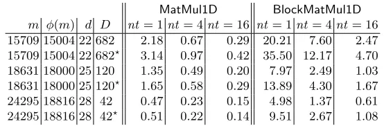
Table 4 shows the effectiveness of parallelization using multiple cores. We show times for both

MatMul1Dand BlockMatMul1D, using 1, 4, and 16 threads. These times are for the default strate-gies, and do not show the time required to build the matrix constants or convert them toDoubleCRT

representation. While the speedups do not quite scale linearly with the number of cores, they are clearly significant, with 16 cores yielding roughly an 8×speedup in large dimensions and 4×speedup in small ones.

We do not present detailed results for the running times of our new implementation of Mat-MulFull and BlockMatMulFull, discussed in Section 7. However, our experiments indicate that the speedups predicted in Section 7 closely align with practice: the speedup forMatMulFullis about the same as our speedup for MatMul1D in the largest dimension; the speedup for BlockMatMulFull is roughly our speedup forBlockMatMul1Din the largest dimension, times the number of dimensions in the hypercube.

Finally, we present some timing results to demonstrate the efficacy of our new algorithms in the context of bootstrapping, as discussed in Section 8. We chose large parameters that demonstrate well the potential saving with our new implementation. Specifically, we used m = 49981 and pr = 2, for which we have φ(m) = 49500 and d = 30. The hypercube structure for Z∗m/(pr) has two dimensions, one of size 150 and one of size 11, for a total of 1650 slots. We note that most parameter choices in [8] attempted to balance the size of the different dimensions, specifically because the linear transformations would take too long otherwise. One of the benefits of our faster algorithms is thus to free us from having to consider that aspect; indeed, our timing shows that the linear transformations are now quite fast even for this “unbalanced” setting.

(24)

bootstrapping and packed bootstrapping routines with both the old and new matrix multiplication algorithms. These results make it clear that for such large hypercubes, thin bootstrapping must be done using our new, faster matrix multiplication to be truly practical.

m φ(m) d D old def new def speedup 15709 15004 22 682 69.28 2.22 31.20 15709 15004 22 682? 138.20 3.14 75.86 18631 18000 25 120 20.27 1.38 14.69 18631 18000 25 120? 39.97 1.69 23.65 24295 18816 28 42 3.18 0.51 6.24 24295 18816 28 42? 6.20 0.55 11.27

Table 1.MatMul1D: summary of old vs new, time in seconds

m φ(m) d D build conv M/B M/F B/BH B/BN B/FH B/FN F/FH F/FN 15709 15004 22 682 0.47 5.54 3.80 44.81 2.22 3.19 6.46 69.28 5.30 28.30 15709 15004 22 682? _{0.56 11.07} _{5.93 44.86} _3.14 _5.03 _{7.33 69.70} _{5.94 29.16} 18631 18000 25 120 0.08 1.96 2.43 13.81 1.38 2.04 2.36 20.27 1.29 8.70 18631 18000 25 120? _{0.10 3.91} _{3.68 13.95} _1.69 _2.89 _{2.45 20.27} _1.29 _8.78 24295 18816 28 42 0.03 0.70 1.39 5.09 0.82 1.17 1.11 6.87 0.51 3.18 24295 18816 28 42? _{0.04 1.39} _{2.17 5.09} _0.95 _1.64 _1.20 _6.94 _0.55 _3.20

Table 2.Different strategies forMatMul1D, time in seconds

m φ(m) d D build conv M/ B/H B/N F/H F/N 15709 15004 22 682 15.47 122.62 54.73 21.03 84.42 18.15 42.67 15709 15004 22 682? 17.31 246.89 64.98 36.81 99.84 32.41 57.07 18631 18000 25 120 2.44 49.59 18.83 9.84 27.90 6.88 14.66 18631 18000 25 120? 2.96 98.79 23.83 17.62 35.80 12.73 20.58 24295 18816 28 42 0.95 19.73 9.25 7.84 13.64 5.01 7.70 24295 18816 28 42? 1.15 39.72 13.49 14.73 20.45 9.65 12.47

(25)

MatMul1D BlockMatMul1D m φ(m) d D nt = 1nt = 4nt = 16 nt= 1nt= 4nt= 16 15709 15004 22 682 2.18 0.67 0.29 20.21 7.60 2.47 15709 15004 22 682? 3.14 0.97 0.42 35.50 12.17 4.70 18631 18000 25 120 1.35 0.49 0.20 7.97 2.49 1.03 18631 18000 25 120? 1.65 0.58 0.29 13.89 4.30 1.67 24295 18816 28 42 0.47 0.23 0.15 4.98 1.37 0.61 24295 18816 28 42? 0.51 0.22 0.14 9.51 2.67 1.08

Table 4.Multithreading forMatMul1DBlockMatMul1D, time in seconds

old new

total linear total linear thin bootstrap 474.18 428.76 80.31 36.17 packed bootstrap 2120.05 804.30 1413.02 102.65

Table 5.Bootstrapping, time in seconds

References

1. J. Alperin-Sheriff and C. Peikert. Practical bootstrapping in quasilinear time. In R. Canetti and J. A. Garay, editors,Advances in Cryptology - CRYPTO’13, volume 8042 ofLecture Notes in Computer Science, pages 1–20. Springer, 2013.

2. Z. Brakerski, C. Gentry, and V. Vaikuntanathan. Fully homomorphic encryption without bootstrapping. In

Innovations in Theoretical Computer Science (ITCS’12), 2012. Available athttp://eprint.iacr.org/2011/277. 3. Z. Brakerski, C. Gentry, and V. Vaikuntanathan. (leveled) fully homomorphic encryption without bootstrapping.

ACM Transactions on Computation Theory, 6(3):13, 2014.

4. H. Chen and K. Han. Homomorphic lower digits removal and improved FHE bootstrapping. In”Advances in Cryptology - EUROCRYPT 2018”, Lecture Notes in Computer Science, pages 315–337. Springer, 2018.

5. C. Gentry. Fully homomorphic encryption using ideal lattices. InProceedings of the 41st ACM Symposium on Theory of Computing – STOC 2009, pages 169–178. ACM, 2009.

6. C. Gentry, S. Halevi, and N. Smart. Fully homomorphic encryption with polylog overhead. In”Advances in Cryptology - EUROCRYPT 2012”, volume 7237 ofLecture Notes in Computer Science, pages 465–482. Springer, 2012. Full version athttp://eprint.iacr.org/2011/566.

7. S. Halevi and V. Shoup. Algorithms in HElib. In J. A. Garay and R. Gennaro, editors,Advances in Cryptology - CRYPTO 2014, Part I, pages 554–571. Springer, 2014. Long version athttp://eprint.iacr.org/2014/106. 8. S. Halevi and V. Shoup. Bootstrapping for HElib. In EUROCRYPT (1), volume 9056 of Lecture Notes in

Computer Science, pages 641–670. Springer, 2015.

9. S. Halevi and V. Shoup. HElib - An Implementation of homomorphic encryption.https://github.com/shaih/ HElib/, September 2014.

10. V. Lyubashevsky, C. Peikert, and O. Regev. On ideal lattices and learning with errors over rings. In H. Gilbert, editor,Advances in Cryptology - EUROCRYPT’10, volume 6110 of Lecture Notes in Computer Science, pages 1–23. Springer, 2010.

11. V. Lyubashevsky, C. Peikert, and O. Regev. ”a toolkit for ring-LWE cryptography”. In T. Johansson and P. Q. Nguyen, editors,Advances in Cryptology - EUROCRYPT 2013, pages 35–54. Springer, 2013.

12. V. Lyubashevsky, C. Peikert, and O. Regev. On ideal lattices and learning with errors over rings. J. ACM, 60(6):43, 2013. Early version in EUROCRYPT 2010.

13. R. Rivest, L. Adleman, and M. Dertouzos. On data banks and privacy homomorphisms. InFoundations of Secure Computation, pages 169–177. Academic Press, 1978.

14. S. Roman. Field Theory. Springer, 2nd edition, 2005.

Faster Homomorphic Linear Transformations in HElib

Faster Homomorphic Linear Transformations in

HElib

Table of Contents