Path Planning of Multiple Mobile Robots

Path Planning of Multiple Mobile Robots

PhD, Assistant Professor, Dept. of Research and Development/ERIS, Batna, Algeria

ABSTRACT: In this paper, we study how and to what extent multiple mobile robots can be guided to in a desired direction to explore an unknown environment and map an area of interest. The scope of the work focuses mainly on the controllers’ design for multiple robots’ path planning and motion coordination. Fuzzy control methodology is developed to: 1. Ensure a best path planning and motion coordination of the mobiles, 2. Avoid the collision and store the position of the obstacles. Genetic algorithm is implemented to optimize the different parameters of the controllers and optimize the robots’ path in case of collision avoidance. To store the obstacle and map the area, the sensors localize the obstacles and store their coordinates in a binary matrix. The algorithms and their implementation are explained in addition to the demonstration of experimental results to illustrate the efficiency and the performances of the study.

KEYWORDS: Path planning, collision avoidance, motion coordination, intelligent control.

I. INTRODUCTION

Many mobile robots have been developed to reduce human activity in hazardous tasks such as explosive ordnance disposal, nuclear material handling, military operation and urban search and rescue; or in exploratory tasks such as Mars’ exploration. Developed robots become an effective tool for human and industry to explore inaccessible places or dangerous areas. With the increasing complexity and diversity of exploiting need, only through the pursuit of some performance indexes of individual robots has been far from meeting the need.

A group of mobile robots moving together in a prescribed pattern can form an efficient data acquisition network for environmental monitoring and exploration. Moreover, path tracking control techniques can be used to perform an interesting aid in dangerous scenes, to perform the mapping of unknown dangerous environment [1][2] [3][4][5].

At present, there are mainly three formation control methods for mobile agents. They are leader-follower method, virtual structure method and behavior method. The basic idea of first method is to make some (usually one) agents be leaders, and the rest be followers. Leaders track the reference path, and followers track the leaders to keep the formation. The second method is to regard the formation as a rigid body, and each agent is relatively fixed in the rigid body. The last method is to divide the formation control task to a set of basic actions, and synthesize the actions to achieve formation control. This whole idea is inspired from the basic management system.

These mobile robots must be fast and effective to allow easy deployment by human operator and yet capable enough to perform many useful functions. They must also be able to last for reasonable operation duration and robust enough to withstand elements that are associated with the mission. A robust lightweight robotic vehicle platform that has a good balance of the abovementioned conflicting requirements has been proposed. It is controlled via wireless communication and modular payloads for specific tasks can be developed at a later stage.

Fig 1. Multiple robots for exploration.

II. PATH PANNING

A. Robot leader controller

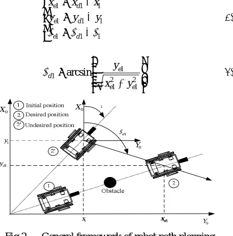
The model of a mobile robot is usually presented in horizontal plane (Figure 2). The robot has the kinematics of a unicycle, described by the well-known equations.

    

  

1 1

1 1 1

1 1 1

sin cos

 

 

  

v y

v x

 

When the robot leader is moving at forward speedv1, the environmental obstacles oblige the robot to deflect from its

desired path. The role of the control system is to keep the system moving as desired by avoiding the obstacles. The idea is to steer the robot such that it eliminates the distance between itself and the desired path just after the collision avoidance (Figure 2).

We define the following variables to mathematically formulate the control objectives:

    

 

 

 

1 1 1

1 1 1

1 1 1

 

_{e d}

d e

d e

y y y

x x x

  

Note that:

 

 

 

 

 

2 1 2

1 1

1 arcsin

e e

e d

y x

y

  

0 Y

1

x

1 d

y

1

y

1



0

X X0

1 d



1 d

x

0

Y

Fig 2. General framework of robot path planning

The fundamental objective is to design the fuzzy controllers to force the robot leader to follow a specified path as closely as possible and the followers as well.

The control input variables for the proposed intelligent controller are chosen as the error e1 and the change of the

error de1 as follows:

  

  

 

) 1 ( ) ( ) (

) ( ) ( ) (

1 1 1

1 1 1

k k k d

k k k

e e e

d e

  

 



 

The variable 1 is defined as the outputs for the fuzzy controller. It is considered as the angle of the motor to change

direction of the mobile robot. We can write:

) , (

Fuzzy 1 1

1 e de

   

Triangular distributions in [1,1] interval are chosen as membership functions for e1(t) ,de1(t) , and1(t).

The defuzzification laws are chosen as shown in Table I.

TABLE I. RULE BASE OF THE FUZZY CONTROLLER

Actuator angle Angle error

NB NM NS ZE PS PM PB

C

h

an

ge

i

n

e

r

ror

PB ZE PS PM PB PB PB PB

PM NS ZE PS PM PB PB PB

PS NM NS ZE PS PM PB PB

ZE NB NM NS ZE PS PM PB

NS NB NB NM NS ZE PS PM

NM NB NB NB NM NS ZE PS

NB NB NB NB NB NM NS ZE

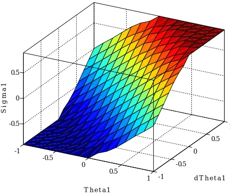
The surface control of the fuzzy controller for the robot leader is presented in figure 3.

-1 -0.5

0 0.5

1 -1 -0.5

0 0.5

1 -0.5

0 0.5

d T h e t a 1

T h e t a 1

S

i

g

m

a

1

Fig 3. Robot leader controller surface

B. Robot Follower Controllers

Suppose there is an arbitrary curve L1 in the X0Y0plane of ground coordinate system, which would be the target path

of leading the robot in the formation. A body frame coordinate system X1Y1 is established for the robot leader moving

According to figure 4, the coordinates of the robotsin the ground coordinate system X0Y0 could be written as:                 2 2 2 2 2 2 2 2 1 1 1 1 1 1 1 1 sin cos : follower Robot sin cos : leader Robot               v y v x v y v x  

In order to satisfy the remaining control goal, the robot follower has to adjust its forward speed and directional angle to coordinate its motion with the robot leader (according to control scheme in figure 6); so as to achieve the desired position and move with the desired velocity profile vd2vd1vd

0 X 0 Y 1 X 1 Y 2 X 2 Y 1  2  1 x 2 x 1 y 2 y 0 X 0 X 1 L 2 L

Fig 4. Coordinate system of path tracking

The desired position of the robot follower with respect to the body frame X1Y1 is defined as:

       y x D y D x 1 2 1 1 2 1   

The objectives of the second controller are to keep 2 1 2 1

, y

x constants and equal to Dx Dy

1 1 _,

respectively, and the

directional angle 2 0

1



e

 in straight motion.

For the robot follower, let’s define the position error with respect to X1Y1:

















The second controller is designed as followed:





TABLE II. RULE BASE OF THE FUZZY CONTROLLER 2 x E B v Z   2 2 ,  N Ex2

Z Ex2

P Ex

 2

N Ey2

N

e2



Z

e2



P

e2

 B v P   2 2 ,  B v P   2 2 ,  B v N   2 2 ,  B v Z   2 2 ,  B v P   2 2 ,  B v N   2 2 ,  B v N   2 2 ,

 2Z,v2B

Z Ey2

P Ey2

B v Z   2 2 ,  B v P   2 2 ,  B v P   2 2 ,  M v P   2 2 ,  M v Z   2 2 ,  M v N   2 2 ,  B v N   2 2 ,  B v N   2 2 ,  B v Z   2 2 ,  S v Z   2 2 ,  S v P   2 2 ,  S v P   2 2 ,  S v N   2 2 ,  S v Z   2 2 ,  S v P   2 2 ,  S v N   2 2 ,  S v N   2 2 ,  S v Z   2 2 ,  e 2  2 y E

 T

v3 3

1



 T

v22

 T

d d d y

x2 , 2 ,2

 T

y x1, 1,1

 T

y x2, 2,2

 T

y x3, 3,3

 T

d d d y

x1 , 1 ,1

 T

d d d y

x3 , 3 ,3

Fig 5. Control scheme of the robot leader and the follower

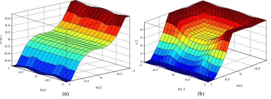
The surface control of the fuzzy controller for the ship follower is presented in figures 6-(a)-(b) for the two outputs 2,v2respectively.

-1 -0.5 0 0.5 1 -1 -0.5 0 0.5 1 -0.6 -0.4 -0.2 0 0.2 0.4 0.6 Ey2 Ex2 S i g 2 -1 -0.5 0 0.5 1 -1 -0.5 0 0.5 1 2 3 4 5 6 Ex2 Ey 2 v 2

III. GENTIC ALGORITHM OPTIMIZATION

In this part, GA is mainly used to design the input/output scaling factors. Genetic algorithm is a robust optimization technique based on natural selection. The basic objective of GA is to optimize fitness function. In genetic algorithms, the term chromosome typically refers to a candidate solution to a problem. GAs have been proved capable of solving large scale or complex problems and they are commonly used as search mechanism when direct search in impossible. Generally, there are three genetic operations in GA: selection, crossover, and mutation. The three operators offer the genes a fine searching mechanism.

After introducing the above operations in GA, the remaining most important thing is the setting of the “Fitness function”.

Various objective functions were written based on error performance criterion. Each objective function is fundamentally the same except for the section of code that defines the specific error performance criterion being implemented.



 e

Ke

 de Kde

v Kdv

d

 x

ExE

K

x dExdE

K

 

y EyE

K

y dEydE

K

.... 2 1oror v



e



de

x

E

x

dE

y

E

y

dE



 K



d

Kd v Kv

     

d d y x

     

y x

  

 

  

 

y x E E e

dt d

dt d

dt d





Fig 7. Genetic algorithm optimization scheme

TABLE III. OBTAINED SCALING FACTORS FOR DIFFERENT GENERATIONS

Type and Parameters 30 generations 50 generations 80 generations

In

p

u

ts

 e

K 0.2915 0.3145 0.3182



de

K 0.0012 0.0015 0.0009

X

E

K 0.0025 0.0019 0.0027

X

dE

K 0.0001 0.0001 0.0001

Y

E

K 0.0021 0.0022 0.0021

Y

dE

K 0.0001 0.0001 0.0001

ou

tp

u

ts

v

K 3.8266 4.1235 4.9512

dv

K 0.0017 0.00021 0.0023



K 0.3911 0.3805 0.4479

 d

K 0.0029 0.0021 0.0031

0 5 10 15 20 25 30 35 40 45 50 0.35

0.4 0.45 0.5 0.55 0.6 0.65 0.7 0.75

t i m e ( s )

F

i

t

n

e

s

s

F

u

n

c

t

i

o

n

30 generations 50 generations 80 generations

Fig 8. Progress of GA that found best fitness for 30, 50, 80 generations

IV. COLLISION AVOIDANCE

The motion of the robot in unknown environment is disturbed by the action of land mines and unpredictable obstacles. Nowadays, a lot of works were done for collision avoidance, and the quality of the results is interesting.

20 30 40 50 60 70 80 90 100 110 120 130 140 150 160 170 180

40 70 100 130 160 190 220

X

Y

Non-Localized obstacles Localized obstacles

Start

End

Fig 9. Robot’s path in mined environment

The collision avoidance system depends on the repulsion theory [7], repulsion from the undesired objects. These objects are classified as follows, rocks, land mines, and borders and already swept areas. The collision avoidance strategy is executed upon the detection of a land mine or an object on front of the robot. The objects are detected with the distance sensor; however the mines are detected by a special detector based on explosive and metal sensors. Figure 9 shows an example for collision avoidance situation.

V. MAPPING AND LOCALIZATION

There are many algorithms and strategies for localizing and mapping the desired area according to the nature of the obstacles. In this paper, mapping and localization is done in a very simple method. As mentioned before the area will be assumed to be square area with Nunits on each side.

                       0 0 0 0 0 0 0 0 0 0 0 0 0 0 0 0 0 1 0 0 1 0 0 0 0 0 0 0 0 0 0 0 0 0 1 0 0 0 0 0 0 0 0 0 0 0 0 0 0 0 0 0 0 0 0 0 1 0 0 0 0 0 0 0 0 0 0 0 0 0 0 0 0 0 0 0 0 0 0 0 0 0 0 0 0 0 0 0 0 0 0 0 1 0 0 0 0 0 0 0 0 0 0 0 0 0 0 0 0 0 0 0 T

VI. SIMULATION RESULTS AND DISCUSSION

The proposed formation control scheme has been implemented in SimulinkTM and simulated for the case of three robots. The desired straight line paths and desired inter-robot spacing is given by(D_x1,D_y1)(0,0),

) 300 , 500 ( ) ,

(D_x2 D_y2    , (D_x3,D_y3)(500,300). The desired velocity profile is chosen as vd 5U .

-500 0 500 1000 1500 2000 2500 3000 3500 4000

-600 -400 -200 0 200 400 600 800 X Y Desired 1 Robot Leader 1 Desired 2 Robot Follower 2 Desired 3 Robot Follower 3

0 100 200 300 400 500 600 700 800

2 2.5 3 3.5 4 4.5 5 5.5 6 6.5 7 time v - f o r w a r d v e l o c i t i e s

Robot Leader 1 Robot Follower 2 Robot Follower 3

Fig 10. Tracking paths of three robots(a), forward velocities(b)

The simulation results are shown in figures 10. Figure 10- (a) shows the trajectories of the robots applying the proposed method of control. Figure 10-(b) shows the variations in the forward velocities.

From the simulation results we know that the leading robot moves to the desired path quickly, and then tracks the path with the forward velocity v1vd 5U; the following robots track the desired path in the respect with the robot leader. During the tracking process, the route, forward velocities and directional angles of each mobile change reasonably.

VII. CONCLUSIONS

The paper presented an approach for land motion coordination. There are four main control behaviors:

1) Robot motion control, 2) Collision avoidance,

3) Localization and mapping, 4) Coordinating the motion of the group.

REFERNECES

[1] Do K. D, Jiang Z. P, Pan J, “Robust and Adaptive Path Following for Underactuated Ships”. Automatica, 40: 929–944, 2004.

[2] Do K. D, Jiang Z. P, Pan J, “Global Partial-State Feedback and Output-Feedback Tracking Controllers for Underactuated Ships”. Systems & Control Letters, 54: 1015–1036, 2005.

[3] Do K. D, Pan J, “Global Robust Adaptive Path Following of Underactuated Ships”. Automatica, 42: 1713–1722, 2006.

[4] Do K.D, Pan J, “Robust Path Following of Underactuated Ships: Theory and Experiments on a Model Ship”. Ocean Engineering, 33: 1354– 1372, 2006.

[5] Enab Y. M, “Intelligent Controller Design for the Ship Steering Problem”, IEE Proceeding Control Theory and, El-Mansoura, Egypt, 143(1): 17–24, 1996.

[6] Even B, Alexey P, Kristin Y. P, “Cross-Track Formation Control of Underactuated Autonomous Underwater Vehicles”. Group Coordination and Cooperative Control, number 336 in ‘Lecture Notes in Control and Information Sciences’, Springer-Verlag, Berlin Heidelberg, 35–54, 2006.

[7] Even B, Alexey P, Reza G, Pettersen, Kristin Y. P, Antonio P, Carlos S, “Formation Control of Underactuated Marine Vehicles with Communication Constraints”. Elsevier IFAC Publications / IFAC Proceedings series, 2006.

[8] Fahimi. F, “Sliding-Mode Formation Control for Underactuated Surface Vessels”. IEEE Transactions on Robotics, 23(3): 617–6222007. [9] Ghabcheloo R, “Coordinated Path Following of Autonomous Vehicles”. PhD Dissertation of Instituto Superior Técnico, Technical University

of Libson. Portugal. May 2007.

[10] Ghabcheloo R, Aguiar A. P, Pascoal A., Silvestre C, Kaminer I, Hespanha J, “Coordinated Path Following in the Presence of Communication Losses and Time Delays”. IEEE Conference on Decision and Control, San Diego, California USA, 2006.