4-18-2012 12:00 AM The Research on the L(2,1)-labeling problem from Graph theoretic and Graph Algorithmic Approaches

(1)

Western University Western University

Scholarship@Western

Electronic Thesis and Dissertation Repository

4-18-2012 12:00 AM

The Research on the L(2,1)-labeling problem from Graph theoretic

and Graph Algorithmic Approaches

Zhendong Shao

The University of Western Ontario

Supervisor

Dr. Roberto Solis-Oba

The University of Western Ontario Graduate Program in Computer Science

A thesis submitted in partial fulfillment of the requirements for the degree in Doctor of Philosophy

Follow this and additional works at: https://ir.lib.uwo.ca/etd

Part of the Computer Sciences Commons

Recommended Citation Recommended Citation

Shao, Zhendong, "The Research on the L(2,1)-labeling problem from Graph theoretic and Graph Algorithmic Approaches" (2012). Electronic Thesis and Dissertation Repository. 494.

https://ir.lib.uwo.ca/etd/494

(2)

The Research on the

L

(2

,

1)-labeling problem from

Graph theoretic and Graph Algorithmic Approaches

(Thesis format: Monograph)

by

Zhendong Shao

Faculty of Science

Department of Computer Science

Submitted in partial fulfillment of the requirements for the degree of

Doctor of Philosophy

School of Graduate and Postdoctoral Studies The University of Western Ontario

London, Ontario April, 2012

c

(3)

THE UNIVERSITY OF WESTERN ONTARIO

SCHOOL OF GRADUATE AND POSTDOCTORAL STUDIES

CERTIFICATE OF EXAMINATION

Advisor Examining Board

Dr. Roberto Solis-Oba Dr. Bin Ma

Dr. Marc Moreno Maza

Dr. Hao Yu

Dr. Kaizhong Zhang

The thesis by Zhendong Shao

entitled

The Research on the L(2,1)-labeling problem from Graph theoretic and Graph Algorithmic Approaches

is accepted in partial fulfillment of the requirements for the degree of

Doctor of Philosophy

(4)

Abstract

Graph coloring is one of the most popular topics in graph theory and many

ad-vances in graph theory are a direct consequence of graph coloring research. The

L(2,1)-labeling problem is a generalization of the vertex coloring problem and its application background is the frequency assignment problem. The L(2,1)-labeling problem has been extensively researched on many graph classes. In this thesis, we

have also studied the problem on some particular classes of graphs.

In Chapter 2 we obtain upper bounds for L(2,1)-labeling numbers of the four standard graph products and get significant improvements over the previously best

known bounds for them.

In Chapter 3 we study theL(2,1)-labeling number of the composition ofngraphs. We show that the L(2,1)-labelling number of the composition of n graphs is much smaller than the square of the maximum degree.

In Chapter 4 we consider the Cartesian sum of graphs and derive, both, lower

and upper bounds for theirL(2,1)-labeling number. We use two different approaches to derive the upper bounds and both approaches improve previously known bounds.

We also present new approximation algorithms for the L(2,1)-labeling problem on Cartesian sum graphs.

In Chapter 5 we characterize d-disk graphs for d > 1, and give the first upper bounds on the L(2,1)-labeling number for this class of graphs.

In Chapter 6 we compute upper bounds for the L(2,1)-labeling number of total graphs ofK1,n-free graphs, whereK1,nis the complete bipartite graph with one vertex in one side of the partition andn in the other.

In Chapter 7 we obtain more results on L(2,1)-labelings of the four standard graph products.

(5)

(6)

Acknowledgments

It is a pleasure to have the opportunity to work with my supervisor, Dr. Roberto

Solis-Oba. Thanks to him for his guidance, encouragement, and support.

Thanks are given to the members of my examining committee, Dr. Bin Ma, Dr.

Marc Moreno Maza, Dr. Hao Yu, and Dr. Kaizhong Zhang.

I am grateful to the faculty and staff members in the Department of Computer

Science for their help.

Last but not least, I would like to thank my parents and my family for their

(7)

List of Figures

1.1 An undirected graph. . . 2

1.2 A directed graph. . . 2

1.3 Complete graphK4. . . 3

1.4 A bipartite graph. . . 4

1.5 Complete bipartite graph K4,3. . . 4

1.6 A graph. . . 5

1.7 A graph of girth 3. . . 5

1.8 A coloring for the vertices of the graph in Figure 7. . . 6

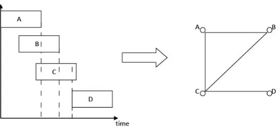
1.9 A set of 4 jobsA, B, C, Dwith conflicting pairs (A, B),(A, C),(B, C),(C, D) and its corresponding graph coloring model. . . 7

1.10 An instance of the register allocation problem and its corresponding graph coloring model. Four variables, A, B, C, and D need to be stored in the registers. When two variables have to be stored at the same time, they conflict. . . 8

1.11 An L(2,1)-labeling for the graph in Figure 7. . . 9

1.12 Cartesian product of graphs P3 and P4. . . 11

1.13 Composition of graphs P3 and P4. . . 12

1.14 Direct product of graphs P3 and P4. . . 13

1.15 Strong product of graphs P3 and P4. . . 14

1.16 Cartesian sum of graphs P3 and P4. . . 15

1.17 The triangular lattice graph Γ(∆), and its disk representation. . . 16

1.18 A graph G and its corresponding total graph. . . 17

1.19 The Mycielski graph µ(K2). . . 18

5.1 Reducing the radius of a circleCi does not decrease the distance from Ci to its neighbouring circles. . . 49

5.2 Angle θ between two neighbouring circles . . . 50

5.3 Spherical sector in 3 dimensions. . . 51

5.4 d-Simplexes4 d and 4 0d. . . 53

(10)

(11)

Chapter 1 Introduction

1.1 Basic Concepts and Notations

In this section we explain some concepts and notations that we use in this thesis. For

a real numbera, we denoteb ac as the largest integer which is not greater thana and

d ae as the smallest integer which is not less thana. For a set S, we denote|S|as the total number of elements in S.

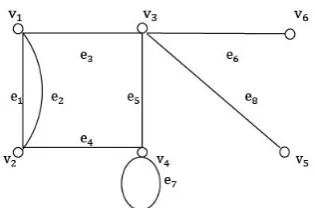
A graph Gis an ordered tuple (V(G), E(G)), where V(G) is an non-empty set of vertices, andE(G) is a set of edges. An edgee= (u, v)∈ E(G) is said to join the two vertices u, v; u, v are called the ends of e. Sometimes we denote an edge (u, v) also as uv. G is called an undirected graph if there is no order between the two vertices

u, v of an edge (u, v), so (u, v) = (v, u); otherwise, G is called a directed graph. See Figure 1.1 for an example of an undirected graph and Figure 1.2 for an example of a

directed graph. Usually, we simply denote a graph as G = (V, E). An edge is called aloop if its two ends are identical; otherwise, it is called alink. Edgee7 in Figure 1.1

is an example of loop. Two edgese1 ande2 are calledmultiple edges if they have the

same endpoints. For example, e1 and e2 in Figure 1.1 are multiple edges. G is called

a simple graph if it has no loops or multiple edges. We usually talk about simple

(12)

Fig. 1.1: An undirected graph.

Fig. 1.2: A directed graph.

The two ends of an edge are said to be incident on the edge. Two vertices are

called adjacent if they are incident on a common edge. The set of vertices which are

adjacent to a vertex u is called the neighborhood of u and is denoted as NG(u). The

degree of u is defined as |NG(u)| and denoted as dG(u). The maximum degree of G, denoted ∆(G), is the largest degree among all vertices in Gand the minimum degree

of G, denoted (_.G), is the smallest degree among all vertices in G. The vertices with degree 0 are calledisolated vertices. For example, the maximum degree of the graph

in Figure 1.1 is 4 and the minimum degree is 1.

Let V(H) ⊆ V(G) and E(H) ⊆ E(G) such that for every edge (u, v) ∈ E(H),

u∈ V(H) andv ∈ V(H), then H = (V(H), E(H)) is called asubgraph ofG, denoted

(13)

as its vertex set and all the edges whose two ends are inV0 as its edge set is called the

subgraph induced byV0, denotedG[V0]. For a nonempty subsetE0 ofE, the subgraph which has E0 as its edge set and the set of ends of edges in E0 as its vertex set is called the subgraph of G induced by E0, denoted G[E0].

LetG1 = (V1, E1), G2 = (V2, E2) be two graphs; the graphG= (V1SV2, E1SE2)

is called the union of G1 and G2 and the graph G= (V1 T

V2, E1 T

E2) is called the

intersection of G1 and G2.

A complete graph is a simple graph such that any two different vertices are

ad-jacent. A complete graph with n vertices is denoted as Kn. See Figure 1.3 for an example of a complete graph. LetV1, V2 be two subsets of the vertex set ofGsuch that

V1SV2 =V(G),V1TV2 =φ, and for which one end of each edge inGis inV1 and the

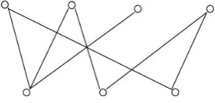
other is inV2, thenGis called abipartite graph, denoted asG= (V1 S

V2, E). See

Fig-ure 1.4 for an example of a bipartite graph. Given a bipartite graphG= (V1SV2, E),

if every vertex in V1 is adjacent to every vertex in V2, then G is called a complete

bipartite graph. A complete bipartite graph G= (V1SV2, E) with |V1|= p,|V2|= q

is denoted as Kp,q. See Figure 1.5 for an example of a complete bipartite graph. If a graph G can be drawn such that its edges only intersect at their ends, then G is called aplanar graph; otherwise, it is called a non-planar graph.

Fig. 1.3: Complete graphK4.

(14)

Fig. 1.4: A bipartite graph.

Fig. 1.5: Complete bipartite graph K4,3.

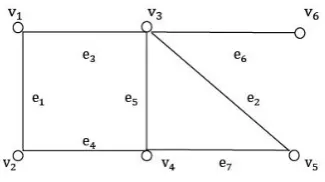
vertices v0, vk are called origin and terminus and integer k is called the length of w. For example, in Figure 1.6, v1e1v2e2v1e3v3e8v5e9v4e5v3e3v1e1v2 is a walk. If all the

edges e1, e2, ...., ek of w are distinct, then w is called a trail. For example, in Figure 1.6, v1e1v2e2v1e3v3e8v5e9v4 is a trail. If all the vertices v1, v2, ...., vk of a trail w are distinct, then w is called a path. For example, in Figure 1.6, v2e1v1e3v3e8v5e9v4 is a

path.

If a walkwhas positive length and its origin and terminus are the same, then it is called closed. If the origin and internal vertices of a closed walk w are distinct, then

w is called a cycle. For example, in Figure 1.6, v1e3v3e5v4e4v2e1v1 is a cycle. If the

length of a cycle is odd, then it is called an odd cycle; otherwise, it is called an even

(15)

Fig. 1.6: A graph.

of the cycle. The girth of a graph G is the length of the shortest cycle in G. For example, the graph in Figure 1.7 is of girth 3.

Fig. 1.7: A graph of girth 3.

If there is a path between vertices uand v, then uand v are said to be connected

and the length of the shortest path between u and v is called the distance between

u and v. Connection is an equivalent relationship on the vertex set V. There is a partition V1, V2, ...., Vb of V such that any two vertices are connected if and only if they belong to the same partitionVk. The subgraphsG[V1], G[V2], ...., G[Vb] are called

components of G. If b= 1, then G is connected.

A subset S of V(G) is called an independent set if and only if no two vertices in

S are adjacent in G. If there is no independent setS0 inG such that|S0|>|S|, then

(16)

maximum independent set. The number of vertices in a maximum independent set

is called the independence numberof G and is denoted as α(G).

A k-vertex proper coloring of G is an assignment of k colors 1,2, ..., k to the vertices of G such that no two adjacent vertices have the same color. G is k-vertex proper colorable if it has ak-vertex proper coloring. The vertex chromatic number of

G, χ(G), is the minimum k such that G is k-vertex proper colorable. For example, the vertex chromatic number of the graph in Figure 1.8 is 3 and the figure shows a

3-vertex proper coloring.

Fig. 1.8: A coloring for the vertices of the graph in Figure 7.

For a subset S of V(G), if G[S] is a complete graph, then S is called a clique of

G.

The adjacency matrixof a graph Gofnvertices is a n× n matrixA = (aij) where the non-diagonal entry aij (i 6=j) is the number of edges from vertex i to vertex j, and the diagonal entries are all equal to zero.

LetA = (aij) be an m× nmatrix and B = (bij) be ap× q matrix, theKronecker

product A⊗ B is the mp× nq block matrix



   

a11B ... a1nB

... ... ... am1B ... amnB



(17)

1.2 Coloring Problems

Graph coloring is one of the most popular topics in graph theory and many advances

in graph theory have been a direct consequence of graph coloring research. The

s-tudy of graph coloring problems can be traced to over one hundred years ago, as these

problems have a large number of applications. For example, the vertex coloring

prob-lem consists in assigning colors to the vertices of a graph so that adjacent vertices are

assigned different colors. This problem can be used, for example, to model scheduling

and register allocation problems. In a scheduling problem the goal is to assign a set

of jobs to a group of machines so as to minimize some objective function, like the

time needed to process them all. Consider, for example, a scheduling problem where

jobs have unit length and there are several pairs of conflicting jobs which cannot be

processed by the same machine. A vertex coloring model for this scheduling problem

can be formulated as follows. Consider a graph whose vertices represent the jobs and

in which there is an edge between any two vertices if the corresponding two jobs

con-flict. The minimum time for the jobs to complete satisfying the conflict restrictions is

just the vertex chromatic number of the above graph. See Figure 1.9 for an example

of this scheduling problem.

(18)

The register allocation problem is to assign a number of variables to a set of

registers; each variable needs to be kept in a register for only a limited amount of

time, and the goal is to find the minimum number of registers needed to store all

the variables. A vertex coloring model can be formulated as follows. Build a graph

whose vertices represent the registers and in which there is an edge between any two

vertices if the corresponding two registers are needed to store variables at the same

time. The minimum number of registers needed is just the chromatic number of this

graph. See Figure 1.10 for an example of the register allocation problem.

Fig. 1.10: An instance of the register allocation problem and its corresponding graph coloring model. Four variables, A, B, C, and D need to be stored in the registers. When two variables have to be stored at the same time, they conflict.

1.3 The

L

(2

,

1)

-Labeling Problem: A Graph

The-oretic Model for the Frequency Assignment

Problem

(19)

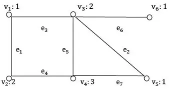
of a graph G is a function f from the vertex set V(G) to the set of all nonnegative integers such that |f(x)− f(y)| ≥ 2 if x and y are adjacent and |f(x)− f(y)| ≥ 1 if

d(x, y) = 2, where d(x, y) denotes the distance between x and y in G. The L(2, 1)-labeling number of G, denoted by λ(G), is the smallest number k such that there is anL(2,1)-labeling with maximum labelk. AnL(2,1)-labeling having maximum label

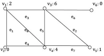
λ is called optimal. For example, the L(2,1)-labeling number of the graph in Figure 1.11 is 6 and 6-L(2,1)-labeling is shown.

Fig. 1.11: An L(2,1)-labeling for the graph in Figure 7.

TheL(2,1)-labeling problem naturally arises from the frequency assignment prob-lem in wireless networks. In the frequency assignment probprob-lem we are given a number

of transmitters or stations and we need to assign a frequency to each one of them

so that transmitters do not interfere with each other. In practice it makes sense to

consider two levels of interference: (1) two ‘very close’ transmitters between which

very strong interference may occur must receive frequencies that differ by at least

two channels, and (2) two ’close’ transmitters must receive different frequencies. The

definition of ’very close’ and ’close’ depends on the physical characteristics of the

transmitters. This problem can be modelled by a graph in which assigning

(20)

minimize the total bandwidth used. Over 100 references on theL(2,1)-labeling prob-lem are provided in a very comprehensive survey [6] by Calamoneri. Due to the

inherent hardness of L(2,1)-labeling problems, most of these papers consider only particular classes of graphs. From the algorithmic point of view it is not surprising

that it is NP-complete to decide whether a given graph G allows an L(2,1)-labeling with maximum label λ(G) [22]. Hence good lower and upper bounds for λ(G) are clearly welcome. For instance, if G is a diameter 2 graph, then λ(G) ≤ ∆2 where ∆ is the maximum degree of G. This upper bound is attainable by Moore graphs

(diameter 2 graphs with ∆2+ 1 vertices), see [22]; such graphs exist for ∆ = 2,3,7, and possibly 57.

In 1992 Griggs and Yeh [22] conjectured that for any graph G with maximum degree ∆ ≥ 2, λ(G) ≤ ∆2_{. Note that this is not true for ∆ = 1 since for example,}

∆(K2) = 1 but λ(K2) = 2. Griggs and Yeh [22] proved that λ≤ ∆2+ 2∆ for general

graphs with maximum degree ∆. Chang and Kuo [10] improved the bound to ∆2_{+ ∆,}

and then Kr´al’ and ˘Skrekovski [34] further reduced the bound to ∆2+ ∆− 1.

Approximation algorithms and inapproximability results for the L(2,1)-labeling problem are rare. In [7], by applying an algorithm by McCormick [40], Calamoneri et

al. proved that there is an algorithm for the L(2,1)-labelling problem with approxi-mation ratio 2((n− 1)1/2 + 1), wheren is the number of vertices in the input graph. In [24], Halldorsson improved the above result by proving that the approximation

ratio of the first-fit algorithm is min{n1/2+ 2,∆} which is the currently best known result. He also proved that it is hard to approximate the L(2,1)-labelling problem within a factor ofn1/2−ε for any ε >0.

In this thesis, we present some of our results in this area and we propose some

interesting open problems. Throughout the document, all graphs are assumed to be

(21)

1.4 The Graph Classes Studied in this Thesis

In this section, we define the various graph classes researched in this thesis. The

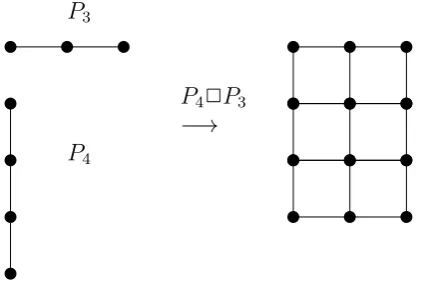
Cartesian product of two graphs G and H is the graph G 2 H with vertex set

V(G)× V(H), in which a vertex (v, w) is adjacent to a vertex (v0, w0) if and only if either v = v0 and w is adjacent to w0 in H or w = w0 and v is adjacent to v0 in G. See Figure 1.12 for an example of the Cartesian product of two graphs.

P3

u u u

u

P4

P42P3

−→

u u u u u u u u u u u u u u u u u u

Fig. 1.12: Cartesian product of graphs P3 and P4.

The composition (or lexicographic product) of two graphs G and H is the graph

G[H] with vertex set V(G)× V(H), in which a vertex (u, v) is adjacent to a vertex (u0, v0) if and only if either uu0 ∈ E(G) or u = u0 and vv0 ∈ E(H). See Figure 1.13 for an example of the composition of two graphs.

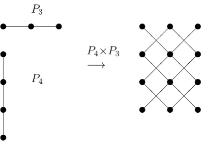
The direct product G× H of two graphs G and H is the graph with vertex set

V(G)× V(H), in which a vertex (v, w) is adjacent to a vertex (v0, w0) if and only if v

is adjacent to v0 in G and w is adjacent to w0 in H. See Figure 1.14 for an example of the direct product of two graphs.

The strong productGH of graphsGandH is the graph with vertex set V(G)×

(22)

P3

u u u

u

P4

P4[P3]

−→

u u u u u u

@ @ @ @ @ @ H H H H H H u u u u u u

@ @ @ @ @ @ H H H H H H

Fig. 1.13: Composition of graphs P3 and P4.

and wis adjacent to w0 in H, or w=w0 and v is adjacent tov0 inG, or v is adjacent tov0 inGand wis adjacent tow0 inH. See Figure 1.15 for an example of this graph product.

The Cartesian sum, GL

H, of two graphsG andH is the graph with vertex set

V(G)× V(H), in which a vertex (u, v) is adjacent to another vertex (u0, v0) if and only if either uu0 ∈ E(G), or vv0 ∈ E(H), or both [44]. See Figure 1.16 for an example of the Cartesian sum of two graphs.

Consider some product G• H of two graphs G and H. Graphs G and H called the factors of the product.

A d-sphere, d≥ 2, is the set of points (x1, x2,· · · , xd) inRdsuch that (x1− c1)2+

(x2− c2)2+· · ·+ (xd− cd)2 =r2, whereris the radiusand (c1, c2,· · · , cd)∈ Rd is the center of the d-sphere. The 2-sphere and 3-sphere are the usual circle and sphere, respectively. The diameter of a sphere of radius r is 2r. A d-sphere with diameter one is called a unit d-sphere.

(23)

P3

u u u

u

P4

P4×P3

−→

u u u u u u

@ @ @ @ @ @ u u u u u u

@ @ @ @ @ @

Fig. 1.14: Direct product of graphs P3 and P4.

overlap. The set D of spheres assigned to the vertices of G is called the disk repre-sentation of G.

Example. The right side of Figure 1.17 shows a 2-disk graph called the triangular lattice graph, Γ(∆), and its disk representation is shown on the left side of Figure

1.17. Γ(∆) is an infinite graph and it is K1,4-free.

Let D be the disk representation of a d-disk graph G. Let dmin and dmax be the minimum and maximum diameters of the d-spheres in D. The value dmax/dmin is called the diameter ratio of D, denoted by σ(D). A disk graph G is called a σ(D )-disk graph if it has a )-disk representation D of diameter ratio σ(D). If σ(D) = 1, then Gis a unitd-disk graph; in this case, we assume that all spheres inD have unit diameter.

Given an undirected graphG= (V, E), thetotal graphT(G) = (V0, E0) ofGis the undirected graph with vertex set V0 = V S

E and edge set E0 = {(u, v)|(u, v) ∈ E, or u = (t, t0) ∈ E and v = (t0, p) ∈ E, or v = (u, t0) ∈ E}. See Figure 1.18 for an example of a total graph.

(24)

P3

u u u

u

P4

P4P3

−→

u u u u u u

@ @ @ @ @ @ u u u u u u

@ @ @ @ @ @

Fig. 1.15: Strong product of graphs P3 and P4.

and edges {(ui, w),(ui, vj)|i, j = 1, ..., n, i 6= j}. See Figure 1.19 for an example of a Mycielski graph. Furthermore, we can recursively define µt₍_G_{) =} _µ₍_µt−1₍_G_{)), for}

t ≥ 2. It is well known that if G is a triangle-free (K3-free) graph then µ(G) is also

triangle-free [64].

1.5 Related Work

The L(2,1)-labeling problem has been extensively studied on many graph classes. We have also studied the problem on several particular classes of graphs. The graph

classes that we have studied are either models for real networks and thus, they have

many potential applications, or they are of theoretical importance. For example,

paths, cycles, and cliques model buses, rings, and mesh networks; these are the

sim-plest and most common networks. The classes of total graphs and Mycielski graphs

are important graph classes widely used as benchmarks in graph coloring problems.

Because many interesting wireless networks have simple factors, such as paths and

cycles and we can gain global information about a network from its factors, product

(25)

P3

u u u

u

u P4

P4LP3

@_@

u u u u u u

@ @ @ @ @ @ H H H H H H u u u u u u

@ @ @ @ @ @ H H H H H H

u u u u u u

@ @ @ @ @ @ A A A A A A A A A A A A A A A A A A A A A A A A B B B B B B B B B B B B B B B B B B

Fig. 1.16: Cartesian sum of graphsP3 and P4.

Cartesian product of n paths, an n-dimensional torus is the Cartesian product of n

cycles, a Hamming graph is the Cartesian product of n copies of the complete graph

K2, and an octagonal grid is the strong product of two paths.

Graph products play an important role in defining various useful types of networks

and they also serve as natural tools for studying different concepts in many areas of

research. For example, one of the central concepts of information theory, the Shannon

capacity, is most naturally expressed with the strong product of graphs [62].

From the viewpoint of human epistemology, it is customary to first devote research

to fundamental concepts and then gradually develop more complex ideas. Research on

the L(2,1)-labeling problem also underwent such a process. For example, researchers first explored labelings on fundamental structures such as paths, circles, and wheels.

Then they focused their research on increasingly more complex structure like

Carte-sian product, composition or lexicographic product, direct product, strong product,

Cartesian sum product of graphs, and so on.

(26)

A A A A A A A A A A A A A A A A A A A A A A A A A A A A A A A A A A A A A A A A A A A A A A A A A A A A A A A A A A A A A A A A A A

Fig. 1.17: The triangular lattice graph Γ(∆), and its disk representation.

( [27], [28], [30], [32], [36] and [47]). L(2,1)-labeling for the Cartesian product of complete graphs has also been considered by Georges et al. [20]. Shao and Yeh [53]

proved that Griggs and Yeh’s conjecture is true for the Cartesian product and the

composition of any two graphs (with minor exceptions).

Jha, Klavˇzar and Vesel [29] considered the direct product of a path and a cycle and

the direct product of two cycles and got bounds for their L(2,1)-labeling numbers. Jha [28] considered the L(2,1)-labeling problem on the strong product of k cycles. Klavˇzar and Spacapan [31] proved that Griggs and Yeh’s conjecture is true for the

direct and strong products of any two graphs. Shao et al. [49] later obtained improved

upper bounds for theL(2,1)-labeling number of the direct and strong products of any two graphs through the use of a refined combinatorial analysis.

Shao and Zhang [57] proved that Griggs and Yeh’s conjecture is true for the

Cartesian sum of any two graphs.

(27)

Fig. 1.18: A graphG and its corresponding total graph.

interference can take place if two transmitters are within a certain distance from each

other. We can model this situation with the so-called interference graphs, which for

this particular example are unit d-disk graphs. Unfortunately, no useful characteri-zation of unitd-disk graphs was known except ford= 1. Using this characterization, Sakai [46] gave upper bounds for the L(2,1)-labeling number of unit 1-disk graphs and proved that these upper bounds corroborate the conjecture of Griggs and Yeh.

Shao et al. [55] characterized unit d-disk graphs for d= 2,3 and gave upper bounds for the L(2,1)-labeling number for this class of graphs.

1.6 Our Contributions

We have several results on L(2,1)-labeling problems, which have been published or have been accepted for publication in reputed scientific journals. We also have some

other work in progress in this area. In the next chapters we present our main results

in this field.

We have obtained some results on product graphs. We have determined both lower

(28)

Fig. 1.19: The Mycielski graph µ(K2).

product ofn graphs and these bounds improve on previously known bounds for these classes of graphs. We also designed approximation algorithms for the Cartesian sum

of any two graphs.

We have been able to characterize unit d-disk graphs for d >3 and d-disk graphs for d > 1, and we found upper bounds on the L(2,1)-labeling number for these two classes of graphs. We were able to show that for these graphs the conjecture of Griggs

and Yeh is true only in some cases.

We computed upper bounds for the L(2,1)-labeling number of total graphs of

K1,n-free graphs, where K1,n is the complete bipartite graph with one vertex in one side of the partition and n in the other. We also determined the exact value for the L(2,1)-labeling number of a class of M ycielski graphs derived from complete graphs and provided lower and upper bounds for the L(2,1)-labeling number of any

M ycielski graph.

1.7 Organization of the Thesis

(29)

In Chapter 2 we present L(2,1)-labelings for the product graphs. In Chapter 3 we present L(2,1)-labelings for the composition of n graphs and in Chapter 4 we present, both, lower and upper bounds for the L(2,1)-labeling number of Cartesian sum graphs. In Chapter 5 we present L(2,1)-labelings of unit d-disk and d-disk graphs. In Chapter 6 we present L(2,1)-labelings of total graphs and in Chapter 7 we present more results onL(2,1)-labelings for the product graphs. In Chapter 8 we present L(2,1)-labelings of Mycielski graphs.

(30)

Chapter 2 L(2,

1)

-Labelings of Product Graphs

Graph products play an important role in connecting various useful networks and

they also serve as natural tools for different concepts in many areas of research. For

examples, the diagonal mesh with respect to multiprocessor network is representable

by the direct product of two odd cycles [61] and one of the central concepts of

in-formation theory, the Shannon capacity, is most naturally expressed with the strong

product of graphs, cf. [62].

The Cartesian product, the lexicographic product, the direct product and the

strong product constitute the four standard graph products [25]. Shao and Yeh

[53] proved that Griggs and Yeh’s conjecture is true for the Cartesian product and

the composition of any two graphs (with minor exceptions) and then Klavˇzar and

Spacapan [31] proved that Griggs and Yeh’s conjecture is true for the direct and strong

products of any two graphs. Recently, Shao, Klavˇzar, Shiu and Zhang [49] improved

the upper bounds obtained in [31] with a more refined analysis of neighborhoods in

product graphs than the analysis in [31].

In this chapter, we study L(2,1)-labelings on the four standard graph products and obtain significant improvements over previously best results.

In the next section a heuristic labeling algorithm is presented that forms the basis

(31)

of graphs are considered, respectively.

2.1 A Labeling Algorithm

A subset X of V(G) is called an i-stable set (or i-independent set), if the distance between any two vertices inX is greater thani. A 1-stable set is a usual independent set. Amaximal i-stable subsetX of a setY of vertices is ani-stable subset ofY such that X is not a proper subset of any other i-stable subset of Y. A maximal i-stable set of a give graph Gcan be computed by using a greedy algorithm: Pick any vertex of G and add it to the i-stable set; remove from G all vertices at distance at most i

from the last vertex selected and then repeat the above procedure as long asG is not empty.

Chang and Kuo [10] proposed the following algorithm to compute an L (2,1)-labeling for a given graph.

Algorithm 2.1.1

Input: A graph G= (V, E).

Output: The valuek of the maximum label.

Idea: In each step, find a maximal 2-stable set from the unlabeled vertices that are at distance at least two from the vertices labeled in the previous step. Label all vertices

in the 2-stable set with the index iof the current step. The indexistarts from 0 and increases by 1 at each step. The maximum label k is the final value of i.

Initialization: Set X−1 =∅ ; V =V(G); i= 0.

Iteration:

1. Determine Yi and Xi.

• IfXi−1 6=∅ then set Yi = {x∈ V : x is unlabeled and d(x, y) ≥ 2 for all

(32)

elseSet Yi =V.

• If Yi 6= ∅ then compute Xi, a maximal 2-stable subset of Yi else set

Xi =∅ .

2. Label the vertices in Xi (if there are any) with i.

3. V ← V\Xi.

4. If V 6=∅ then seti← i+ 1 and go to Step 1.

5. Record the current value of i as k (which is the maximum label). Stop.

Note that the value k computed by the above algorithm is an upper bound on

λ(G). We would like to find a bound fork in terms of the maximum degree ∆(G) of

G, analogous to existing bounds for the chromatic number χ(G) in terms of ∆(G). Let x be a vertex with the largest label k assigned by Algorithm 2.1.1. Denote

• I1 = {i : 0 ≤ i ≤ k− 1 and d(x, y) = 1 for some y ∈ Xi}. This is the set of labels of the neighbors of x.

• I2 = {i : 0 ≤ i ≤ k− 1 and d(x, y)≤ 2 for some y ∈ Xi}. This set consists of the labels of the vertices at distance at most 2 from x.

• I3 ={i: 0≤ i≤ k− 1 and d(x, y)≥ 3 for all y∈ Xi}. This set consists of the labels not used by vertices at distance at most 2 from x.

It is clear that|I2|+|I3|=k. For anyi∈ I3,x /∈ Yi since otherwiseXi∪{ x} would be a 2-stable subset of Yi, which contradicts the choice of Xi. That is, d(x, y) = 1 for some vertex y in Xi−1; i.e., i− 1 ∈ I1. Since for every i ∈ I3, i− 1 ∈ I1, then

|I3| ≤ |I1|. Hencek =|I2|+|I3| ≤ |I2|+|I1|.

(33)

B =|I1|+|I2| (2.1)

in terms of ∆(G).

2.2 The Cartesian Product of Graphs

In [53], they obtained an upper bound on λ(G2H) in terms of the maximum degree of G2H for any two graphs G and H. In this section, we also consider this problem.

Theorem 2.2.1 Let∆1 and∆2 be maximum degrees of GandH, respectively. Then

λ(G2H)≤ ∆2

1+ ∆22+ ∆1∆2+ ∆1 + ∆2.

Proof. We first apply Algorithm 2.1.1 to label the graph G2H and let k be the maximum label obtained by the algorithm. Letx= (u, v) inV(G)×V(H) be a vertex with the label k. Then degG2H(x) = degG(u) +degH(v). Denote d = degG2H(x),

d1 = degG(u), d2 = degH(v), ∆1 = ∆(G) and ∆2 = ∆(H). Hence d = d1 +d2 and

∆ = ∆(G2H) = ∆1+ ∆2.

Let G = (V, E) be a graph. Let A be its adjacency matrix with respect to the list of vertices {v1, . . . , vn}. Then it is well-known that the (i, j)th entry of Ak is the number of different (vi− vj)-walks in G of length k, for k ≥ 0. Thus, the number of the nonzero entries in the i-row ofA2 _{is the number of vertices of distance 2 from} _v

i

(it includes the vertex vi itself if deg(vi)6= 0).

Let the order ofGandHbeν1andν2, respectively. SupposeV(G) ={u1, . . . , uν1}

and V(H) = {v1, . . . , vν2}. Consider the cartesian product graphG2H. We list the

vertex setV(G)× V(H) in lexicographic order. Then the adjacency matrix of G2H

(34)

matrices of Gand H respectively, I1 and I2 are the identity matrices of orderν1 and

ν2 respectively. Note thatP ⊗ Q is the Kronecker product of the matrices P and Q.

Then A2+A=A2₁⊗ I2+ 2A1 ⊗ A2+I1⊗ A22+A1⊗ I2+I1⊗ A2.

For fixed vertex (ui, vj) in G2H, the number of nonzero entries in the (ui, vj)th row of A2 +A excluding the diagonal entries is the same as the number of nonzero entries in the (ui, vj)th row ofA21⊗ I2+A1⊗ A2+I1⊗ A22+A1⊗ I2+I1⊗ A2 excluding

the diagonal entries.

For fixed vertex (ui, vj) in G2H, we only look at the (ui, vj)th row of the above matrix. Then the number of nonzero entries in this row excluding the diagonal entries

is at most

deg_G(ui)(∆1− 1) + degG(ui) degH(vj) + degH(vj)(∆2− 1) + degG(ui) + degH(vj) = deg_G(ui)∆1+ degH(vj)∆2+ degG(ui) degH(vj).

Thus, λ(G2H)≤ |I2|+|I1| ≤ ∆21 + ∆22+ ∆1∆2+ ∆1+ ∆2.

The above result agrees with the result in [53].

2.3 The Composition of Graphs

In [53], they provided an upper bound on λ(G[H]) in terms of the maximum degree of G[H] for any two graphs G and H. In this section, we also consider this problem.

Theorem 2.3.1 Let ∆1 and ∆2 be maximum degrees of G and H, respectively. Let

ν2 be the number of vertices of H. Then λ(G[H])≤ ∆12ν2+ ∆22− 1 + ∆1ν2+ ∆2.

Proof. Again, we apply Algorithm 2.1.1 to obtain an L(2,1)-labeling with the maximum labelkon the graphG[H]. Supposex= (u, v)∈ V(G)×V(H)(=V(G[H])) is labeled by k. Denote d1 = degG(u), d2 = degH(v), ∆1 = ∆(G), ∆2 = ∆(H) and

(35)

Let G and H be two graphs of order ν1 and ν2, respectively. Suppose V(G) =

{u1, . . . , uν1} and V(H) = {v1, . . . , vν2}. Consider the composition graph G[H]. We

list the vertex set V(G)× V(H) in lexicographic order. Then the adjacency matrix of G[H] with respect to this list is A = A1 ⊗ J2 +I1 ⊗ A2, where A1 and A2 are

adjacency matrices of G and H respectively, J2 is the square matrix of order ν2 all

of whose entries are equal to 1 and I1 is the identity matrix of order ν1. Note that

P ⊗ Qis the Kronecker product of the matrices P and Q. Then A2₊_A₌_ν

2A21⊗ J2+A1⊗ J2A2+A1⊗ A2J2+I1⊗ A22+A1⊗ J2+I1⊗ A2

=ν2A21⊗ J2+A1⊗ (J2A2+A2J2+J2) +I1 ⊗ A22+I1⊗ A2

For fixed vertex (ui, vj) in G[H], the number of nonzero entries in the (ui, vj)th row of A2 +A excluding the diagonal entries is the same as the number of nonzero entries in the (ui, vj)th row of A21 ⊗ J2+A1 ⊗ J2+I1⊗ A22 +I1 ⊗ A2 excluding the

diagonal entries.

Let ∆1 and ∆2 be the maximum degrees of G and H, respectively. For fixed

vertex (ui, vj) in G[H], we only look at the (ui, vj)th row of the above matrix. Then the number of nonzero entries in this row excluding the diagonal entries is at most

deg_G(ui)(∆1− 1)ν2+ degG(ui)ν2+ degH(vj)(∆2− 1) + degH(vj) = degG(ui)∆1ν2+

deg_H(vj)∆2.

Thus, |I2|+|I1| ≤ ∆21ν2+ ∆22− 1 + ∆1ν2 + ∆2.

In [53] it was proved that λ(G[H])≤ ∆2_{+ ∆}₋ ₂_ν 2∆1.

Because ∆2+∆−2ν2∆1−(∆21ν2+∆22−1+∆1ν2+∆2) = ∆21ν2(ν2−1)+2∆1(∆2−1)ν2,

we reduce the bound by ∆2

1ν2(ν2− 1) + 2∆1(∆2 − 1)ν2.

2.4 The Direct Product of Graphs

(36)

Theorem 2.4.1 Let∆1 and∆2 be maximum degrees of GandH, respectively. Then

λ(G× H)≤ ∆2

1∆22− ∆21∆2− ∆1∆22+ 3∆1∆2.

Proof. Again, we apply Algorithm 2.1.1 to obtain an L(2,1)-labeling with the maximum label k on the graph G× H. Let x = (u, v) in V(G)× V(H). Then deg_G_×_H(x) = deg_G(u)deg_H(v). Denote d = deg_G_×_H(x), d1 = degG(u), d2 = degH(v), ∆1 = ∆(G) and ∆2 = ∆(H). Hence d=d1d2 and ∆ = ∆(G× H) = ∆1∆2.

{u1, . . . , uν1} and V(H) = {v1, . . . , vν2}. Consider the direct product graph G× H.

We list the vertex setV(G)×V(H) in lexicographic order. Then the adjacency matrix of G× H with respect to this list is A = A1 ⊗ A2, where A1 and A2 are adjacency

matrices of G and H respectively. Note that P ⊗ Q is the Kronecker product of the matrices P and Q.

Then A2₊_A₌_A2

1⊗ A22+A1⊗ A2.For fixed vertex (ui, vj) inG× H, the number of nonzero entries in the (ui, vj)th row of A2 +A excluding the diagonal entries is the same as the number of nonzero entries in the (ui, vj)th row of A21⊗ A22+A1⊗ A2

excluding the diagonal entries.

Let ∆1 and ∆2 be the maximum degrees ofGandH, respectively. For fixed vertex

(ui, vj) in G× H, we only look at the (ui, vj)th row of the above matrix. Then the number of nonzero entries in this row excluding the diagonal entries is at most

deg_G(ui)(∆1− 1) degH(vj)(∆2− 1) + degG(ui) degH(vj).

Thus, |I2|+|I1| ≤ ∆1(∆1 − 1)∆2(∆2 − 1) + 2∆1∆2 = ∆21∆22 − ∆21∆2 − ∆1∆22+

3∆1∆2.

In [49] it was proved that λ(G× H)≤ ∆2_{+ ∆}₋ _(∆

1+ ∆2)(∆1 − 1)(∆2− 1).

Because ∆2_{+ ∆}₋ _(∆

1+ ∆2)(∆1− 1)(∆2− 1)− (∆21∆22− ∆21∆2−∆1∆22+ 3∆1∆2) =

∆2

(37)

2.5 The Strong Product of Graphs

In [28] the λ-numbers of the strong product of cycles were considered. In [31] and [49], they obtained upper bounds for the λ-number of strong products in terms of the maximum degree of GH for any two graphs G and H. In this section, we also consider this problem.

Theorem 2.5.1 Let ∆1 and ∆2 be the maximum degree of G and H, respectively.

Then λ(GH)≤ ∆2

1∆22+ ∆21+ ∆22+ ∆1∆2.

Proof. Again, we apply Algorithm 2.1.1 to obtain an L(2,1)-labeling with the maximum label k on the graph G H. Let x = (u, v) in V(G)× V(H). Then deg_G_H(x) = deg_G(u) + deg_H(v) + deg_G(u)deg_H(v). Denote d = deg_G_H(x), d1 =

deg_G(u), d2 = degH(v), ∆1 = ∆(G) and ∆2 = ∆(H). Hence d =d1+d2+d1d2 and

∆ = ∆(GH) = ∆1 + ∆2+ ∆1∆2.

{u1, . . . , uν1} and V(H) = {v1, . . . , vν2}. Consider the strong product graph GH.

We list the vertex setV(G)×V(H) in lexicographic order. Then the adjacency matrix of GH with respect to this list is A=A1⊗ A2+A1⊗ I2+I1⊗ A2, where A1 and

A2 are adjacency matrices of G and H respectively, J2 is the square matrix of order

ν2 all of whose entries are equal to 1 and I1 is the identity matrix of order ν1. Note

that P ⊗ Qis the Kronecker product of the matrices P and Q.

Then A2+A = (A1⊗ A2)2+ (A1⊗ I2+I1⊗ A2)2+A1⊗ A2(A1⊗ I2+I1⊗ A2) +

(A1⊗ I2+I1⊗ A2)A1⊗ A2+A1 ⊗ A2 +A1 ⊗ I2+I1⊗ A2 = A12⊗ A22+A21 ⊗ I2+

2A1⊗ A2+I1⊗ A22+ 2A21 ⊗ A2+ 2A1⊗ A22 +A1⊗ A2+A1 ⊗ I2+I1⊗ A2

For fixed vertex (ui, vj) in GH, the number of nonzero entries in the (ui, vj)th row of A2 +A excluding the diagonal entries is the same as the number of nonzero entries in the (ui, vj)th row ofA21⊗ A22+A21⊗ I2+ 2A1⊗ A2+I1⊗ A22+ 2A21⊗ A2+

(38)

Let ∆1 and ∆2 be the maximum degrees ofGandH, respectively. For fixed vertex

(ui, vj) in GH, we only look at the (ui, vj)th row of the above matrix. Then the number of nonzero entries in this row excluding the diagonal entries is at most

deg_G(ui)(∆1 − 1) degH(vj)(∆2 − 1) + degG(ui)(∆1 − 1) + degG(ui) degH(vj) + deg_H(vj)(∆2− 1) + degG(ui)(∆1− 1) degH(vj) + degG(ui) degH(vj)(∆2− 1) +

deg_G(ui) degH(vj) + degG(ui) + degH(vj). Thus,

|I2|+|I1| ≤ ∆1(∆1− 1)∆2(∆2− 1) + ∆1(∆1− 1) + ∆1∆2+ ∆2(∆2− 1) + ∆1(∆1−

1)∆2+ ∆1∆2(∆2− 1) + ∆1∆2+ ∆1+ ∆2 = ∆21∆22+ ∆21+ ∆22+ ∆1∆2.

In [49] it was proved that λ(GH)≤ ∆2+ ∆− (∆1+ ∆2 + 4)∆1∆2∆2 + ∆1+

∆2− 5∆1∆2.

Because ∆2+ ∆− (∆1+ ∆2+ 4)∆1∆2− (∆21∆22+ ∆21+ ∆22+ ∆1∆2) = (∆1+ ∆2−

(39)

Chapter 3 L(2,

1)

-Labelings of the

Composition of

n

Graphs

Graph products play an important role in network applications. In [53] the Cartesian

product and the composition of two graphs were studied and it was proven that

the L(2,1)-labeling number of these graphs is bounded above by the square of the maximum degree (with minor exceptions); unfortunately, the proof for the bound

on the L(2,1)-labeling number of the composition of graphs had a mistake, so the bound is only valid for graphs with no isolated vertices. In this chapter we address

the problem with the proof in [53] and study the L(2,1)-labeling number of the composition of n graphs. We show that the L(2,1)-labelling of the composition of n

graphs is much smaller than the square of the maximum degree. As corollaries, our

bound for the L(2,1)-labeling number of the composition of n graphs is better than that given in [60] for the composition of two graphs G1[G2] if ν2 <∆22+ 1, where ν2

(40)

3.1 The Combinatorial Analysis Approach

The definition of the composition of two graphsGandH has been provided in Section 1.4.

By the definition of G[H], if ∆(G) = 0, then G[H] consists of disjoint copies of

H. Thus λ(G[H]) =λ(H). Therefore, we assume ∆(G)≥ 1.

The composition of n (n≥ 2) graphs G1, G2, ..., Gn, CG1,G2,...,Gn, is defined

recur-sively byCGn =Gnand CGk,Gk+1,...,Gn =Gk[CGk+1,Gk+2,...,Gn] fork =n− 1, n− 2, ...,1.

In this section, we obtain an upper bound for λ(CG1,G2,...,Gn) in terms of the

maximum degrees ofG1, G2, ..., Gn, CG1,G2,...,Gn.

Theorem 3.1.1 Let G1, G2, ..., Gn be graphs with maximum degrees∆1, ∆2, ..., ∆n,

respectively, such that ∆1 ≥ 1. Then

λ(CG1,G2,...,Gn)≤ β2(1 + ∆1+ ∆

2

1) +α− 1,

where βj = |V(Gj)| × |V(Gj+1)| × · · · × | V(Gn)| for all j = 1,2, . . . , n, and α =

Pn−1

j=2(βj+1∆j) + ∆n.

Proof. Let us apply Algorithm 2.1.1 to CG1,G2,...,Gn and let x = (i1, i2, . . . , in) ∈ V(CG1,G2,...,Gn) be a vertex with the largest label. Let d be the degree of x in

CG1,G2,...,Gn and for each j = 1,2, . . . , n, let us define the following values: dj is

the degree of ij in Gj, νj = |V(Gj)| , and βj = νjνj+1· · ·νn. Let βn+1 = 1. Note

from the definition of composition that the number of vertices of CGj,...,Gn is βj, for

all j = 1,2, . . . , n. Let t be the number of vertices at distance 2 from vertex x in graph CG1,...,Gn.

Observe that graph CGj,...,Gn, j < n, can be constructed as follows:

1. Replace each vertex uof Gj with a copy of CGj+1,...,Gn. Let us denote this copy

of CGj+1,...,Gn corresponding to vertexu as C

u_.

(41)

Therefore, the set of the following vertices contains all the vertices of CG1,G2,...,Gn

that are at distance two from x= (i1, i2, . . . , in): The vertices in the copy Ci1 _of _C

G2,...,Gn corresponding to vertex i1, with the

exception of x and the neighbours of x in Ci1_{. The number of vertices in} _Ci1 _is

ν2ν3· · ·νn and the number of neighbours of x in Ci1 is d− d1ν2ν3· · ·νn as d is the total number of neighbours of x and d1ν2ν3· · ·νn is the number of neighbours of x that do not belong to Ci1_.

There can be at most d1(∆1 − 1)ν2ν3· · ·νn vertices not in Ci1 at distance 2 from

x as each neighbour of i1 inG1 has at most ∆1 neighbors.

Hence,

t ≤ ν2ν3· · ·νn− (d− d1ν2· · ·νn)− 1 +d1(∆1− 1)ν2· · ·νn = ν2· · ·νn(1 +d1∆1− d1)− d+d1ν2· · ·νn− 1

= β2(1 +d1∆1)− d− 1

The maximum degree of the graph CG1,G2,...,Gn is

∆ = n

X

j=1

(βj+1∆j) = β2∆1+

n

X

j=2

(βj+1∆j)

= β2∆1+α, where α=

n

X

j=2

(βj+1∆j). (3.1)

Thus, we obtain the following boundB for theL(2,1)-labelling number ofCG1,G2,...,Gn

(42)

B = |I1|+|I2| ≤ d+d+t

≤ 2d+β2(1 +d1∆1)− d− 1

= d+β2(1 +d1∆1)− 1

≤ ∆ +β2(1 +d1∆1)− 1

= β2∆1+α+β2(1 +d1∆1)− 1, by (3.1)

= β2(1 + ∆1+d1∆1) +α− 1.

Corollary 3.1.2 LetG, H be graphs with maximum degrees ∆1, ∆2 respectively, such

that ∆1 ≥ 1. Then

λ(G[H])≤ β2(1 + ∆1+ ∆21) +α− 1 = ν2∆1+ ∆2− 1 +ν2(1 + ∆21).

In [60], Shiu et al. proved that λ(G[H]) ≤ ν2∆1 + ∆2 +ν2∆21 + ∆22. Because

ν2∆1+ ∆2+ν2∆21+ ∆22− (ν2∆1+ ∆2− 1 +ν2(1 + ∆12)) = ∆22− ν2+ 1,the bound in

Corollary 3.2.2 is better than that of Shiu et al. if ν2 <∆22+ 1.

Lemma 3.1.3 Let G1, G2 be graphs with maximum degrees ∆1, ∆2 and numbers of

vertices ν1, ν2, respectively, such that ∆1 = 2 and∆2 = 0. Then λ(G1[G2])≤ 5ν2− 1.

In particular, λ(C5[G2]) = 5ν2− 1, where C5 is a cycle with 5 vertices.

Proof. Without loss of generality, we can suppose that G1 =Cν1, i.e., G1 is a cycle

with ν1(ν1 ≥ 3) vertices. We give an explicit (5ν2− 1)-L(2,1)-labeling l for G1[G2].

Letv0, ..., vν1−2 be vertices of Cν1 such that vi is adjacent tovi+1,0≤ i≤ ν1− 2 and

v0 is adjacent to vν1−1. Then, consider the following cases:

Case 1. ν1 ≡ 0 mod 3.

Subcase 1. i ≡ 0 mod 3. Label each vertex in each copy of G2 in G1[G2]

(43)

corre-sponding to vi with labels ν2+ 1, ν2+ 2, ...,2ν2.

corre-sponding to vi with labels 2ν2+ 2,2ν2+ 3, ...,3ν2+ 1.

Case 2. ν1 ≡ 1 mod 3. First we label each vertex in the copy of G2 in G1[G2]

corresponding to v0, ..., vν2−2 as follows

Subcase 1. i ≡ 0 mod 3. Label each vertex in the copy of G2 in G1[G2]

corre-sponding to vi with labels 0,1, ..., ν2 − 1.

corre-sponding to vi with labels 2ν2+ 2,2ν2+ 3, ...,3ν2+ 1.

corre-sponding to vi with labels ν2+ 1, ν2+ 2, ...,2ν2.

Finally, label each vertex in the copy ofG2 inG1[G2] corresponding tovν2−1 with

labels 3ν2+ 2,3ν2+ 3, ...,4ν2+ 1.

Case 3. ν1 ≡ 2 mod 3. First we label each vertex in the copy of G2 in G1[G2]

corresponding to vertices v0, ..., vν2−3 as follows

corre-sponding to vi with labels 0,1, ..., ν2 − 1.

Subcase 2. i≡ 1 mod 3. First label each vertex except the last one in the copy of

G2 inG1[G2] corresponding to vi with labels ν2+ 1, ν2+ 2, ...,2ν2− 1 and then label

the last vertex with 4ν2.

corre-sponding to vi with labels 2ν2+ 1,2ν2+ 2, ...,3ν2.

Finally label each vertex in the copy of G2 in G1[G2] corresponding to vν2−2 as

follows: First, label each vertex except the last one in this copy of G2 with labels

4ν2+ 1,4ν2+ 2, ...,5ν2− 1 and then label the last vertex with labelν2. Finally, label

each vertex in the copy of G2 in G1[G2] corresponding to vν2−1 as follows: first label

(44)

and then label the last vertex with label 2ν2.

It is easy to verify that the above labeling is a valid L(2,1)-labeling for G1[G2]

and, therefore, λ(G1[G2])≤ 5ν2 − 1.

Note that since C5 is a diameter 2 graph, then C5[G2] is also a diameter 2 graph,

therefore all vertices of C5[G2] must be assigned different labels. Thus, λ(C5[G2])≥

5ν2 − 1. But since we already showed that λ(C5[G2]) ≤ 5ν2 − 1, then λ(C5[G2]) =

5ν2 − 1. Hence, the above labelling scheme is optimal for C5[G2].

Lemma 3.1.4 Let G1, G2 be graphs with maximum degrees ∆1, ∆2 and numbers of

vertices ν1, ν2, respectively, such that∆1 ≥ 1 and ∆2 = 0. Then λ(CG1,G2)≤ ∆

2₋ _∆

where ∆ is the maximum degree of CG1,G2, with the only exceptions that λ(CG1,G2)≤

∆2_{+ ∆} _when _∆

1 ≥ 3 and ν2 = 1 and λ(CG1,G2) = ∆

2 _when_C

G1,G2 consists of copies

of C4.

Proof. Because ∆2 = 0, the number of vertices at distance one fromxis at mostν2∆1

and the number of vertices at distance two fromx is at most ν2∆1(∆1− 1) +ν2− 1.

Hence, we can compute the bound B from euqation (2.1) as follows: |I1| ≤ ν2∆1,

|I2| ≤ ν2∆1+ν2∆1(∆1− 1) +ν2− 1. ThenB =|I1|+|I2| ≤ ν2∆1+ν2∆1+ν2∆1(∆1−

1) +ν2− 1 =ν2∆21+ν2∆1+ν2− 1. We need to consider three cases.

Case 1. ∆1 ≥ 3.

Subcase 1. ν2 = 1. Then CG1,G2 = G1. In this case, CG1,G2 is the general graph

G1 with maximum degree ∆1 ≥ 3.

Subcase 2. ν2 ≥ 2. Since (ν2∆1)2 − ν2∆1− (ν2∆21 +ν2∆1+ν2 − 1) = ν2((ν2 −

1)∆2

1 − 2∆1 − 1) + 1 ≥ ν2(9ν2− 16) + 1 = 9ν22 − 16ν2 + 1 ≥ 2ν2 + 1. Hence B ≤

(ν2∆1)2− ν2∆1− (2ν2+ 1) = ∆2 − ∆− (2ν2+ 1).

Case 2. ∆1 = 2. By Lemma 3.2.3, we haveλ(G1[G2])≤ 5ν2− 1.

But

(ν2∆1)2−ν2∆1−(5ν2−1) = 4ν22−7ν2+1≥ 3, soλ(G1[G2])≤ (ν2∆1)2−ν2∆1−3 =

(45)

Case 3. ∆1 = 1. Then λ(G1[G2]) = 2ν2.

If ν2 ≥ 3, then (ν2∆1)2− ν2∆1− 2ν2 =ν22− 3ν2 ≥ 0.Hence λ(G1[G2])≤ ∆2− ∆.

If ν2 = 2, then G1[G2] consists of copies of C4. Hence λ(G1[G2]) = 4≤ ∆2.

Lemma 3.1.5 Let G1, G2, ..., Gn be graphs with maximum degrees ∆1, ∆2, ..., ∆n,

respectively, such that ∆1 ≥ 1. Then λ(CG1,G2,...,Gn) ≤ ∆

2 ₋ _∆_{, where} _∆ _{is the}

maximum degree ofCG1,G2,...,Gn, with the only exceptions that λ(CG1,G2,...,Gn)≤ ∆

2_+∆

when ν2 =ν3 =· · · =νn = 1 and λ(CG1,G2,...,Gn) = ∆

2 _where _C

G1,G2,...,Gn consists of

copies of C4.

Proof. From Theorem 3.2.1, λ(CG1,G2,...,Gn) ≤ β2(1 + ∆1 + ∆

2

1) +α− 1 so we just

need to show that this bound is at most ∆2− ∆, except when ν2 =ν3 =· · ·=νn = 1 orCG1,G2,...,Gn consists of copies ofC4. Note that

∆2− ∆− (β2(1 + ∆1+ ∆21) +α− 1)

= (β2∆1+α)2 − (β2∆1+α)− (β2(1 + ∆1+ ∆12) +α− 1), from (3.1)

= (β₂2− β2)∆21+ 2β2∆1(α− 1) +α2− 2α− β2+ 1

We now need to consider three cases.

Case 1. α=Pn

j=2(βj+1∆j) = 0. Then ∆j = 0, j = 2, ..., n. By Lemma 3.2.3, the

conclusion holds.

Case 2. α=Pn

j=2(βj+1∆j) = 1. Then

Subcase 1. β2 = 1. Sinceβ2 =ν2ν3· · ·νn = 1, thenν2 =ν3 =· · ·=νn= 1. Hence

CG1,G2,...,Gn = G1. In this case, CG1,G2,...,Gn is the general graph G1 with maximum

degree ∆1 ≥ 1.

Subcase 2. β2 ≥ 2. Since ∆2− ∆− (β2(1 + ∆1+ ∆21) +α− 1) = (β22− β2)∆21+

2β2∆1(α−1)+α2−2α−β2+1 = (β22−β2)∆12−β2 =β2((β2−1)∆12−1)≥ β2(∆21−1)≥ 0.

(46)

Case 3. α = Pn

j=2(βj+1∆j) ≥ 2. Then ∆

2 ₋ _∆₋ ₍_β

2(1 + ∆1+ ∆21) +α− 1) =

(β2

2− β2)∆21+2β2∆1(α− 1)+α2−2α−β2+1≥ (β22−β2)∆21+β2(2∆1− 1)+1≥ β22+1(

since β2 ≥ 2 and ∆1 ≥ 1). Then the conclusion holds.

By the proof of Lemma 3.2.5, the bound in Theorem 3.2.1 is much smaller than

∆2− ∆ ifα≥ 2 or if α= 1 and ∆1 ≥ 2.

3.2 Correction to the Proof in [53] for the

Com-position of Two Graphs

Theorem 4.3 in [53] states a bound for λ(CG1,G2) by establishing a lower bound on

ε, the number of edges of the subgraph F induced by the neighbors of a vertex x

labelled with the largest label by algorithm Label. Unfortunately, the proof of the

theorem given in [53] is not totally correct because if vertexx is isolated inG2, then

the lower bound for ε will not hold and therefore the upper bound forλ(G1[G2]) can

not be established by this method but if vertexxis not isolated inG2, then the lower

bound for ε will still hold and therefore the proof is still correct. In this section, we fix the proof of that Theorem.

Theorem 3.2.1 [53] Let the maximum degree of G1[G2] be ∆. Then λ(G1[G2]) ≤

∆2+ ∆− 2ν2∆1 or λ(G1[G2])≤ ∆2 − ∆, with the only exceptions that λ(CG1,G2)≤

∆2_{+ ∆} _when _∆

1 ≥ 3 and ν2 = 1 and λ(G1[G2]) = ∆2 when G1[G2]consists of copies

of C4.

Proof. We use Algorithm 2.1.1 to obtain an L(2,1)-labeling with maximum label k

for the graph G1[G2]. Let x∈ V(G1[G2]) be labeled byk. We only consider the case

when the degree of x inG2 is zero.

Case 1. ∆2 >0. Because x is isolated in G2, the number of vertices at distance

(47)

most ν2∆1(∆1− 1) +ν2− 1. Hence for computing the bound B from equation (2.1)

we get |I1| ≤ ν2∆1, |I2| ≤ ν2∆1 +ν2∆1(∆1 − 1) +ν2 − 1. Then B = |I1|+|I2| ≤

ν2∆1+ν2∆1+ν2∆1(∆1− 1) +ν2− 1 = ν2∆21+ν2∆1+ν2− 1.

Since ∆2 >0 andx is isolated in G2,ν2 ≥ 3. Note that ∆1 ≥ 1 and ∆2 ≥ 1, then

(ν2∆1+ ∆2)2− (ν2∆1+ ∆2)− (ν2∆12+ν2∆1+ν2− 1) =ν2((ν2 − 1)∆21+ 2∆1(∆2−

1)) + ∆2(∆2− 1) +ν2− 1≥ ν2(ν2− 1)∆21+ν2− 1≥ ν2(ν2− 1) +ν2− 1 =ν22− 1≥ 8.

Hence B ≤ (ν2∆1+ ∆2)2− (ν2∆1+ ∆2)− (ν22− 1) = ∆2− ∆− (ν22− 1)≤ ∆2− ∆− 8.

(48)

Chapter 4 On Some Results for the

L(2,

1)

-Labeling on Cartesian Sum

Graphs

In [53], [31] and [57], Shao and Yeh, Klav˘zar and ˘Spacapan, and Shao and Zhang

proved that the L(2,1)-labeling number of the Cartesian product, the composition, the direct product, the strong product and the Cartesian sum of graphs is bounded by

the square of the maximum degree (with minor exceptions). Shao, Klavˇzar, Shiu and

Zhang [49] improved the upper bounds obtained in [31] with a more refined analysis

of neighborhoods in product graphs than that used in [31].

In this chapter we consider the Cartesian sum of graphs and derive, both, lower

and upper bounds for the L(2,1)-labeling number; we use two approaches to derive the upper bounds and both approaches improve previously known bounds. We also

(49)

4.1 Lower and Upper Bounds on the

L

(2

,

1)

-Labelings

of Cartesian Sum Graphs

Given a graph G, the number of vertices in G is denoted ν(G). A vertex u of G is isolated if its degree is zero. The number of isolated vertices in G is denoted t(G). The maximum degree of Gis denoted ∆(G). If u and v are two adjacent vertices of

G, the edge connecting them is denoted as uv.

Lemma 4.1.1 LetGand H be two graphs. ThenGL

H has a subgraph of diameter two with (ν(G)− t(G))(ν(H)− t(H)) vertices and it also has a subgraph of diameter three with max{ν(G)(ν(H)− t(H)), ν(H)(ν(G)− t(G))} vertices.

Proof. Let G0 and H0 be the subgraphs of G and H obtained by removing all the isolated vertices, respectively. Observe that if G0 or H0 are empty then the first bound of the Lemma holds trivially, so let us assume that G0 and H0 are not empty. Let G0 and H0 consist of connected components G1, G2, ..., Gk (k ≥ 1) and

H1, H2, ..., Hp (p ≥ 1), respectively. Note that ν(Gi) ≥ 2 and ν(Hj) ≥ 2 for each connected component Gi, Hj, i = 1,2, ..., k, j = 1,2, ..., p. Let (u, v),(u0, v0) be any two nonadjacent vertices of GL

H, where u ∈ Gi, v0 ∈ Hl, for i ∈ { 1,2, ..., k} and

l ∈ { 1,2, ..., p}. Since Gi and Hl are connected, let u00 be a vertex adjacent to u in

Gi and let v00 be a vertex adjacent to v0 in Hl. By the definition of GLH, (u, v) and (u00, v00) are adjacent and (u0, v0) and (u00, v00) are also adjacent. Hence (u, v) and (u0, v0) are at distance two in GL

H, and so GL

H has a subgraph G0L

H0 of diameter two with (ν(G)− t(G))(ν(H)− t(H)) vertices.

We now derive the first part for the second bound of the Lemma. Note that if H0

is empty this part of the bound is trivially zero, so we assume that H0 is not empty. Let (u, v),(u0, v0) be two nonadjacent vertices of GL

H, where u ∈ Gi, u0 ∈ Gj and

(50)

and Gj are connected, let u00 be a vertex adjacent to u in Gi and let u000 be a vertex adjacent to u0 in Gj. By the definition of G

L

H, (u, v) and (u00, w) are adjacent, (u000, w0) and (u0, v0) are adjacent, and (u00, w) and (u000, w0) are adjacent. Hence (u, v) and (u0, v0) are at distance three. Then G0L

H has a subgraph of diameter three that includes G0 and all vertices of H; this subgraph hasν(H)(ν(G)− t(G)) vertices. Similarly,GL

H0 has a subgraph of diameter three withν(G)(ν(H)− t(H)) vertices.

Corollary 4.1.2 LetG andH be two connected graphs. ThenGL

H is of diameter two.

Theorem 4.1.3 For any two graphs G and H, λ(GL

H)≥ (ν(G)− t(G)) (ν(H)− t(H))− 1.

Proof. By Lemma 4.1.1, GL

H has a subgraph of diameter two with (ν(G)−

t(G))(ν(H)− t(H)) vertices. Since in an L(2,1)-labeling of a diameter two graph all the vertices must have different labels, then λ(GL

H) ≥ (ν(G)− t(G))(ν(H)−

t(H))− 1.

We now compute an upper bound for λ(GL

H).

Theorem 4.1.4 For any two graphsGandH, λ(GL

H)≤ ν(G)ν(H)− t(G)t(H) + ∆(GL

H)− 1.

Proof. Note thatGL

Hhast(G)t(H) isolated vertices. Thus, the number of vertices within distance two from any vertexx, is at mostν(G)ν(H)−t(G)t(H)−1. Therefore, by Algorithm 2.1.1,λ(GL

H)≤ |I2|+|I1| ≤ ν(G)ν(H)− t(G)t(H) + ∆(G L

H)− 1.

In [57] it is proved thatλ(GL

H)≤ D0 = (∆(GL

H))2−ν(G)(∆(G)−1)∆(H)−

(51)

ν(G)ν(H)− t(G)t(H) + ∆(GL

H)− 1, be the bound from Theorem 4.1.4. We now compare the bounds D0 and D.

Note that ∆(GL

H) =ν(G)∆(H) +ν(H)∆(G)− ∆(G)∆(H)≥ 2(ν(G)

ν(H)∆(G)∆(H))1/2₋_∆(_G_)∆(_H_{) = (∆(}_G_)∆(_H₎₎1/2₍₂₍_ν₍_G₎_ν₍_H₎₎1/2₋_(∆(_G_)∆(_H₎₎1/2_{) =}

(∆(G)∆(H))1/2₍₍_ν₍_G₎_ν₍_H₎₎1/2_{+ (}_ν₍_G₎_ν₍_H₎₎1/2₋

(∆(G)∆(H))1/2₎_≥ _(∆(_G_)∆(_H₎₎1/2₍₍_ν₍_G₎_ν₍_H₎₎1/2_{+ (∆(}_G_)∆(_H_{) + ∆(}_G_{) + ∆(}_H_{) +}

1)1/2 ₋ _(∆(_G_)∆(_H₎₎1/2₎ _> _(∆(_G_)∆(_H₎₎1/2₍_ν₍_G₎_ν₍_H₎₎1/2_{, the second inequality}

fol-lows from ν(G)≥ ∆(G) + 1 and ν(H)≥ ∆(H) + 1. Thus, (∆(GL

H))2 _{> ν}₍_G₎_ν₍_H_)∆(_G_)∆(_H_{) and so}

D0−D= [(∆(GL

H))2₋_ν₍_G_)(∆(_G₎₋_1)∆(_H₎₋_ν₍_H_)(∆(_H₎₋_1)∆(_G₎₋_(∆(_G₎₊

∆(H))∆(G)∆(H)− ∆(G) − ∆(H) + 1] − [ν(G)ν(H) − t(G)t(H) + ∆(GL

H) −

1] = [(∆(GL

H))2 ₋ _ν₍_G_)(∆(_G₎₋ _1)∆(_H₎ ₋ _ν₍_H_)(∆(_H₎ ₋ _1)∆(_G₎ ₋ _(∆(_G_{) +}

∆(H))∆(G)∆(H)− ∆(G) − ∆(H) + 1]− [ν(G)ν(H) − t(G)t(H) + (ν(G)∆(H) +

ν(H)∆(G)−∆(G)∆(H))−1] = (∆(GL

H))2₋₍_ν₍_G₎_ν₍_H₎₋_t₍_G₎_t₍_H₎₎₋₍_ν₍_G_)∆(_G_)∆(_H₎₊

ν(H)∆(H)∆(G)+(∆(G)+∆(H)−1)∆(G)∆(H)+∆(G)+∆(H)−2)> ν(G)ν(H)∆(G)∆(H)−

(ν(G)ν(H)− t(G)t(H))− (ν(G)∆(G)∆(H) +ν(H)∆(H)∆(G) + (∆(G) + ∆(H)−

1)∆(G)∆(H) + ∆(G) + ∆(H)− 2).

Noting again that ν(G) ≥ ∆(G) + 1 and ν(H) ≥ ∆(H) + 1, we conclude that

D0 − D = Θ(ν(G)ν(H)∆(G)∆(H)). So, our bound is asymptotically better than in [57].

4.2 Algorithm BlockLabel

In this section, we present a different algorithm for computing an L(2,1)-labeling for the Cartesian sum of two graphs that is better than the algorithm presented in the

Section 4.1.

(52)

with the minimum possible number of colors so that adjacent vertices have different

colors. The minimum number of colors needed to color the vertices of a graph G

is called the chromatic number of G, denotedχ(G). Consider two graphs G, H and optimum coloringsχG,χH for them. Without loss of generality, let the colors assigned to the vertices of G and H be 1, ..., χ(G) and 1, ..., χ(H) respectively; moreover, let all the isolated vertices in G and H be assigned color 1. We partition the vertices of

GL

H into blocks, as follows. All vertices (u, v) of GL

H where u has color i and

v has color j are placed in block Bij. LetB be the set of all these blocks. We use the following algorithm for labeling GL

H.

Algorithm BlockLabel(B)

Input: Set B of blocks as described above.

Output: The maximum label used in anL(2,1)-labeling for the vertices inB.

1. Sort the blocks in B in any order. 2. l← 0.

3. For each block Bij ∈ B do { 4. If i= 1 andj = 1 then {

5. For each vertex u∈ B11 do{

6. Ifu is isolated in GL

H then Assign u label 0. 7. otherwise Assignu label l and then set l← l+ 1.

} }

8. otherwise

9. For each vertex u∈ Bij do Assignu label l and then set l← l+ 1. 10. l ← l+ 1//skip a label.

}

(53)

Theorem 4.2.1 Let G and H be two graphs. Then one of the following holds. a. If both G and H are not complete graphs or odd cycles, then λ(GL

H) ≤

ν(G)ν(H)− t(G)t(H) + ∆(G)∆(H)− 2;

b. If both G and H are odd cycles, then λ(GL

H)≤ ν(G)ν(H) + 7;

c. If both G and H are complete graphs, then λ(GL

H) = 2ν(G)ν(H)− 2;

d. If one ofGandHis not a complete graph or odd cycle, but the other is an odd cycle, then λ(GL

H)≤ ν(G)ν(H) + 3∆(G)− 2 or λ(GL

H)≤ ν(G)ν(H) + 3∆(H)− 2;

e. If one of G and H is not a complete graph or odd cycle, but the other is a complete graph, then λ(GL

H) ≤ ν(G)ν(H) + ∆(G)ν(H) − 2 or λ(GL

H) ≤

ν(G)ν(H) + ∆(H)ν(G)− 2;

f. If one of G and H is a complete graph and the other is an odd cycle, then

λ(GL

H)≤ ν(G)ν(H) + 3ν(G)− 2 or λ(GL

H)≤ ν(G)ν(H) + 3ν(H)− 2.

Proof. We first show that algorithm BlockLabel produces an L(2,1)-labeling for

GL

H. Let us consider the non-isolated vertices in some block Bij ∈ B. For any two vertices (u, v) and (u0, v0) in Bij, since uand u0 have the same color iinχG, then

u and u0 are at distance at least two in G; similarly,v and v0 are at distance at least two in H. By the definition of GL

H, (u, v) and (u0, v0) are at distance at least two inGL

H. Thus, all the vertices in block Bi,j can be labelled consecutively.

Now let us consider the vertices in two different blocks. For any two vertices

(u, v) and (u0, v0) from two different blocks of B, there is the possibility that they are adjacent in GL

H. Note that since in algorithm BlockLabel at least one label has been skipped between the labelling of (u, v) and (u0, v0), then the labels of these vertices differ by at least 2 and so the above labelling scheme is feasible.

The number of labels used to label GL

H is equal to the number ν(G)ν(H)−

t(G)t(H) of non-isolated vertices plus the number of labels skipped in step 10 of the algorithm. Notice that the number of labels skipped is equal to the number of blocks

inB minus 1.

Since the number of blocks inB is at mostχ(G)χ(H), thenλ(GL

4-18-2012 12:00 AM The Research on the L(2,1)-labeling problem from Graph theoretic and Graph Algorithmic Approaches

Scholarship@Western

Scholarship@Western

The Research on the L(2,1)-labeling problem from Graph theoretic

The Research on the L(2,1)-labeling problem from Graph theoretic

and Graph Algorithmic Approaches

and Graph Algorithmic Approaches

The Research on the

L

(2

,

1)-labeling problem from

Graph theoretic and Graph Algorithmic Approaches

(Thesis format: Monograph)

Zhendong Shao

Faculty of Science

Department of Computer Science

Abstract

Acknowledgments

Contents

List of Figures

Chapter 1

Introduction

1.1

Basic Concepts and Notations

1.2

Coloring Problems

1.3

The

L

(2

,

1)

-Labeling Problem: A Graph

The-oretic Model for the Frequency Assignment

Problem

1.4

The Graph Classes Studied in this Thesis

1.5

Related Work

1.6

Our Contributions

1.7

Organization of the Thesis

Chapter 2

L(2,

1)

-Labelings of Product Graphs

2.1

A Labeling Algorithm

2.2

The Cartesian Product of Graphs

2.3

The Composition of Graphs

2.4

The Direct Product of Graphs

2.5

The Strong Product of Graphs

Chapter 3

L(2,

1)

-Labelings of the

Composition of

n

Graphs

3.1

The Combinatorial Analysis Approach

3.2

Correction to the Proof in [53] for the

Com-position of Two Graphs

Chapter 4

On Some Results for the

L(2,

1)

-Labeling on Cartesian Sum

Graphs

4.1

Lower and Upper Bounds on the

L

(2