Article
A Decision Support Tool for Teacher Assignment
Problem
Ngo Tung Son1,*, Bui Ngoc Anh1, Jafreezal Jaafar2
1 Information and Communication Technology Department, FPT University, Hanoi 100000, Vietnam;
[email protected]; [email protected];
2 Department of Computer and Information Sciences, Center for Research in Data Science, Universiti
Teknologi PETRONAS, Tronoh 32610, Malaysia; [email protected]; * Correspondence: [email protected]
Abstract: The problem of scheduling is an area that has attracted a lot of attention from researchers for many years. Its goal is to optimize resources in the system. The assigning task to the lecturer is an example of the timetabling problem, a class of scheduling. In this study, we introduce a mathematical model to assign fixed tasks (the time and required skills to be fixed) to university lecturers. Our model is capable of generating a calendar that maximizes faculty expectations. The formulated problem is in the form of a multi-objective problem that optimal makes decisions require the trade-off presence of trade-offs between two or more conflicting objectives. To solve this, we use different approaches to multi-objective programming. We then proposed the installation of the Genetic Algorithm to solve the introduced model. Finally, the model and algorithm tested with real scheduling data collected at the Computing Fundamental Department, FPT University, Hanoi, Vietnam.
Keywords: Timetabling, Task Assignment, MOP, Combinatory Optimization, Compromise Programming, Genetic Algorithm.
1. Introduction
1.1. Background
The need to optimize types of resources is as much a requirement in training organizations as in any other kind of institution. The goal of the university timetabling problem is to find a method to allocate the predefined resources that minimize the cost where all constraints within the problem must be satisfied. The resources here consist of classes meant to be a group of students with the same schedule, a subject that requires one or more specific skills and knowledge, time slots that determine when a particular class and subject attached. The university usually performs a scheduling task before a semester begins [1, 2, 3, 4, 5].
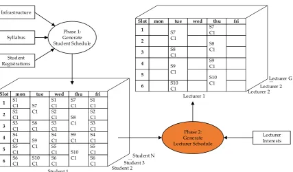
This research conducted on a practical case study at FPT University in Vietnam. Currently, the university's scheduling process is a semi-automatic process. Now, the university's scheduling process is a semi-automatic process. In the situation, the student can register for their studies very soon before the head of the department has enough resources to determine the final schedule (of course, some classes could be canceled due to lack of resources later). The system creates groups of students who would like to study the same subject based on the registrations and selects the time slots for these groups automatically. However, the department heads still manually assign their lecturer to teach these classes later. The reason for this is that we are student-centered, other resources revolve around students to support them. The problem becomes an instance of the teaching assignment problem [6]. This study aims to provide an automated task assigning to replace the manual process highlighted by the orange-colored ellipse in Figure 1.
Syllabus Student Registrations 1 2 3 4 5 6 S1 C1 S2 C1 S3 C1 S4 C1 S5 C1 S6 C1 S7 C1 S8 C1 S9 C1 S10 C1 S1 C1 S2 C1 S3 C1 S4 C1 S5 C1 S6 C1 S7 C1 S8 C1 S9 C1 S10 C1 S1 C1 S2 C1 S3 C1 S4 C1 S5 C1 S6 C1
Slot mon tue wed thu fri
Student 2 Student 3...
Student N Infrastructure 1 2 3 4 5 6 S7 C1 S8 C1 S9 C1 S10 C1 S7 C1 S8 C1 S9 C1 S10 C1
Slot mon tue wed thu fri
... Phase 1: Generate Student Schedule Phase 2: Generate Lecturer Schedule Student 1
Lecturer 1 Lecturer 2
Lecturer 2 Lecturer G
Lecturer Interests
Figure 1: The training schedule process at FPT University that contains two phases. The manual stage highlighted with orange.
The input data for the decision-making stage described as Every class established for a particular subject and took place in 30-time slots (equivalent to 45 hours of study, 1-time slots is equal to 1.5 hours). A student can join a maximum of ten classes, but only one class per time-slot. The duration of a semester is ten weeks. Every class has three slots of the same subject per week and must not take place for two consecutive days, which aims to give the student time to prepare for the next sections. Each semester the university opens about 1000 classes. Lecturers can teach a maximum of 6 slots per day. Table 1 illustrates ten available time-slots for a teacher/student for every week in the semester.
Table 1: The details of 10-time slots defined at the FPT University for a week.
DoW Time-Slot
Monday Tuesday Wednesday Thursday Friday Part of the day
1 M1 M4 M1 M4 M1 Morning
2 M2 M4 M2 M5 M2
3 M3 M5 M3 M5 M3
4 E1 E4 E1 E4 E1 After Noon
5 E2 E4 E2 E5 E2
6 E3 E5 E3 E5 E3
1.2. Related Work
dimensions of one container and the lectures as different sized items then assign them into the container [8].
Task assignment problems come in many different forms. While some of them like the classical problem have polynomial-time solutions [9], others are NP-hard combination optimization problems [10] that requires heuristic approaches [11]. In [12], Lewis classifies several metaheuristic-based techniques into three classes for University Timetabling problems in their survey. Muthuraman and Venkatesan also conducted a survey of meta-heuristic algorithms for solving the combinatorial optimization problems [13]. They reviewed several algorithms such as ant colony optimization, evolutionary computation, particle swarm optimization etc. Related to the scheduling problem, many researchers used genetic algorithms, an evolutionary algorithm to solve scheduling problems, as well as task assignment problems [14,15,16]. Genetic Algorithm generates high-quality solutions to optimization and search problems. A particular researcher can have different design of the Genetic Algorithm to solve specific problems. Feng et al combine genetic algorithms and search strategies to create offspring in populations based on information collected from the best individuals of previous generations and with a local search that improves the efficacy of the proposed Genetic Algorithm [17]. Yang develops an efficient hybrid genetic algorithm based on algorithms for the converted problem [8]. In this study, we introduce a binary integer optimization problem and a version of the Genetic Algorithm to solve the task assignment problem that mentioned in section 1.1.
1.3. Contribution
In this study, we present an approach to construct a task assignment support system for the university. The work we perform is not only a stage in the automatic scheduling solution at FPT University but also a new approach for the problem of the fixed-tasks assignment. The related researches to the scheduling may benefit from our study. Due to the fixed schedule that respects the business requirement, the considered events such as classes, time-slots, and subjects determined. Our mission is to arrange the available works for available human resources. We built a multi-objectives model that accesses the level of interest of each individual assigned to the job, which still provides a binding compliance solution. The formulation of the problem described in section 2. There are many ways to solve the proposed optimization model. We present two approaches, linear scalazing and compromising, to transform the multi-objective problem into a single-objective problem. Each method has its advantages and disadvantages and is suitable for different decision-maker groups. We have implemented a genetic algorithm that solves both optimal models of a target mentioned above—the detail of the implementation described in section 3. In the following sections of this paper, we present the results of our experiments using the scheduling data of Computer Fundamentals at FPT University. A review of the two algorithms also discussed in section 4. The remaining are discussion and conclusion.
2. Problem Formulation
2.1. Multi-Objective Task Assignment Problem
Many researchers have used integer programming (IP) model to solve this type of problem such as [1, 3]. In this research, we also define our timetable problem in form of IP as following:
• Let 𝐺 is the number of lecturers.
• Denote 𝑆 is the number of subjects.
• 𝑇 is the number of available time slots, in our case, 𝑇 = 10 as described in Table 1.
• 𝐻 is the number of section, a section represents a particular class studies a specific subject at a timeslot.
• 𝑐ℎ, 𝑠ℎ, 𝑡ℎ are class, subject and time slot of section ℎ𝑡ℎ respectively.
• 𝐷𝑔 is a number of classes that lecturer 𝑔𝑡ℎ prefer to teach.
• 𝑎𝑠,𝑔 ≥ 0 as integer for every 𝑠 = 1 … 𝑆, 𝑔 = 1. . 𝐺 represent the rating of the lecturer 𝑔𝑡ℎ to teach subject 𝑠𝑡ℎ. The value 0 indicates that the lecturer does not want to teach the subject.
Other values respectively mean “like a little” to “like very much”.
• 𝑏𝑡,𝑔 ≥ 0 as integer for every 𝑡 = 1 … 𝑇, 𝑔 = 1. . 𝐺 denote the rating of the lecturer 𝑔𝑡ℎ to teach at time slot 𝑡𝑡ℎ. The value 0 indicates that the lecturer does not want to teach at the
time slot. Other values respectively mean “like a little” to “like very much”.
• 𝑥ℎ,𝑔 is the decision variable for every ℎ = 1 … 𝐻, 𝑔 = 1 … 𝐺. 𝑥ℎ,𝑔= 1 if the lecturer 𝑔𝑡ℎ is assigned to section ℎ𝑡ℎ, 𝑥
ℎ,𝑔= 0 otherwise.
In [18], Corne suggested some of timetabling constraints such as (1) Unary constraints, (2) Binary constraints, (3) Capacity constraints, (4) Event spread constraints, (5) Agent constraints. Based on those suggestions, we also define several constraints to the problem as follows:
• All section must be assigned lecturer and at most one lecturer is assigned to a section.
∑ 𝑥ℎ,𝑔
𝐺
𝑔=1
= 1 ∀𝑠𝑠 = 1 … 𝐻 (𝐻1)
• A particular lecturer does not teach the subject that he/she does not have skill.
𝑎𝑠ℎ,𝑔≥ 𝑥ℎ,𝑔 ∀ℎ = 1 … 𝐻, 𝑔 = 1 … 𝐺 (𝐻2)
• A particular lecturer does not teach at the time-slot that he/she is not available.
𝑏𝑡ℎ,𝑔≥ 𝑥ℎ,𝑔 ∀ℎ = 1 … 𝐻, 𝑔 = 1 … 𝐺 (𝐻3)
• All lecturers have to satisfy the quota for the number of sections they have to teach.
∑ 𝑥ℎ,𝑔
𝐻
ℎ=1
≥ 𝑀𝑔 ∀𝑔 = 1 … 𝐺 (𝐻4)
In the past, several researchers proposed models focused on assignments for rooms and time slots to achieve workable schedules while optimizing the lecturer's interests. For example: Nouri and Driss [19, 20] use the multi-agent approach, where the agents represent teachers of different levels and seek to assign their lectures according to their interests. Higher-ranking teachers are given priority in meeting their interests. Malik et al build a model for mapping the task to the lecturer that maximizes the preference of the time-slot [21]. There are many different views about the compact schedule. The goal is to avoid idle time on the teacher's plan and to minimize the number of working days [22,23]. In this research we have defined some objectives functions that maximizes the preferences level of the lecturer on time-slots, subjects and the number of classes that the lecturer want to teach. The objective functions described as follows:
• Maximize the expectations of the lecturers on the subject they want to teach.
max {∑ 𝑥ℎ,𝑔∗ 𝑎𝑠ℎ,𝑔
𝐻
ℎ=1
} ∀𝑔 = 1 … 𝐺 (∗)
• Maximize the expectations of the lecturers on the time slots they want to teach.
max {∑ 𝑥ℎ,𝑔∗ 𝑏𝑡ℎ,𝑔
𝐻
ℎ=1
} ∀𝑔 = 1 … 𝐺 (∗∗)
• Minimize the errors on the number of classes that the lecturers want to teach.
min {|∑ 𝑥ℎ,𝑔− 𝐷𝑔
𝐻
ℎ=1
|} ∀𝑔 = 1 … 𝐺 (∗∗∗)
• Minimize the number of parts of the day, which lecturers have to work (morning, afternoon every day). The lecturer would register three classes, even if he expressed his interest in all of the time-slots. It is better to assign him/her to work in the slot-times (E1, E2, E3) instead of (E1, E4, M1):
max{𝑝𝑜𝑑({𝑥ℎ,𝑔| ℎ = 1. . 𝐻})} ∀𝑔 = 1 … 𝐺 (∗∗∗∗)
Where 𝑝𝑜𝑑 is a fuzzy logic membership function that return the rating for the number of parts of the day, which lecturers have to work.
approach to transform the optimal problem into a more suitable form so that we can find the optimal solution in the decision space.
2.2. Approaches for MOP
Our proposed scheduling problem becomes a MOP. There are two main approaches to solving the MOP problem: preference method and non-preference method, mentioned in the survey of Hwang [25]. The most useful solution found using different philosophies that depending on the subjective preferences of the decision-makers. Here, the decision-maker plays an important role. The solutions need to revolve around them. In this section of this paper, we discuss the linear scalarization, an instance of preference method, and another is a compromised approach that requires no pre-defined preferences of the decision-maker.
2.2.1. Linear Scalarization
Scalarizing a MOP means formulating a single-objective optimization problem such that optimal solutions to the single-objective optimization problem are Pareto optimal solutions to the multi-objective optimization problem [25]. It may require some parameters of the scalarization to reach the Pareto optimal solution [26]. The original multi-objective functions (*), (**), (***) and (****) rewritten in form of linear Scalarizing as:
max ∑ (𝛼𝑔(∑ 𝑥ℎ,𝑔∗ 𝑎𝑠ℎ,𝑔
𝐻
ℎ=1
) + 𝛽𝑔(∑ 𝑥ℎ,𝑔∗ 𝑏𝑡ℎ,𝑔
𝐻
ℎ=1
) + 𝛾𝑔
1
1 + |∑𝐻ℎ=1𝑥ℎ,𝑔− 𝐷𝑔|
𝐺
𝑔=1
+ 𝛿𝑔𝑝𝑜𝑑({𝑥ℎ,𝑔| ℎ = 1. . 𝐻}) )
Where 𝛼𝑔, 𝛽𝑔, 𝛾𝑔, 𝛿𝑔 ∀𝑔 = 1 … 𝐺 are float numbers, denote the weight of the objective function 𝑔𝑡ℎ on respectively the group of objectives (*), (**), (***) and (****).
In the decision-making process, decision-makers can place interest in each criterion according to his / her subjective preferences. Here, the decision-maker should be an expert in the domain. It is challenging to find the desired weights.
2.2.2. Compromise Programming
The problem of 4*g objective functions is complicated for decision-makers to define the weights corresponding to each lecturer. There are many proposed methods to solve multi-objective problems. Zeleny [27] introduced the ideal solution that defined as the best-compromise solution that is the nearest to the perfection. Ngo et al [28, 29, 30] applied compromise programming to solve the binary objectives problem in team selection, where they introduced the idea point 𝐸 and try to find the solution that has minimum distance to 𝐸. When the decision maker stands in the view of lecturers, they declare their preferences on subjects and time-slots. It is hard to find the solution to archive the best but we can define the best schedule they expect. The only goal left is to find a solution that is closest to this predefined point. We called those considerations as dimension of interest. The objective function now expressed as follow:
• Denote 𝐸 ∈ ℝ𝐺×(𝑇+2)= {𝐸
1, 𝐸2, … , 𝐸𝐺} is the matrix of idea timetable.
Where 𝐸𝑔= {𝐸𝑔,1, 𝐸𝑔,2, … , 𝐸𝑔,𝑇, 𝐸𝑔,𝑇+1, 𝐸𝑔,𝑇+2} is the vector of expected timetable for lecturer
𝑔𝑡ℎ, such that
𝐸𝑔,𝑗 = {
max
ℎ=1..𝐻∣𝑡ℎ=𝑗 (𝑎𝑠ℎ,𝑔∗ 𝑏𝑗,𝑔) 𝑖𝑓 𝑗 ≤ 𝑇
𝑛𝑜𝑟𝑚(𝐷𝑔) 𝑖𝑓 𝑗 = 𝑇 + 1
ℶ 𝑜𝑡ℎ𝑒𝑟𝑤𝑖𝑠𝑒
Where 𝑛𝑜𝑟𝑚 denotes the normalization function, ℶ is max rating for the number of parts of the days that a lecturer has to work.
• Let 𝐹 is the matrix of the solution. 𝐹 ∈ ℝ𝐺×(𝑇+2)= {𝐹
1, 𝐹2, … , 𝐹𝐺} where 𝐹𝑔=
𝐹𝑔,𝑗=
{
∑ 𝑥ℎ,𝑔∗ 𝑎𝑠ℎ,𝑔∗ 𝑏𝑗,𝑔
𝐻
ℎ=1∣𝑡ℎ=𝑗
𝑖𝑓 𝑗 ≤ 𝑇
𝑛𝑜𝑟𝑚 (∑ 𝑥ℎ,𝑔
𝐻
ℎ=1
) 𝑖𝑓 𝑗 = 𝑇 + 1
𝑝𝑜𝑑({𝑥ℎ,𝑔| ℎ = 1. . 𝐻}) 𝑜𝑡ℎ𝑒𝑟𝑤𝑖𝑠𝑒
The original multi-objective functions (*), (**), (***) and (****) rewritten in form of compromise problem (CP):
min(𝑑𝑖𝑠𝑡𝑎𝑛𝑐𝑒([𝐸1, 𝐸2, … , 𝐸𝐺], [𝐹1, 𝐹2, … , 𝐹𝐺])) = √∑ ∑(𝐸𝑖,𝑗− 𝐹𝑖,𝑗)
2 𝑇+2
𝑗=1 𝐺
𝑖=1
3. Proposed Algorithm
3.1. Introduction to Genetic Algorithm
The Genetic Algorithm [31] is a population-based heuristic method extensively used in scheduling problems. It searches a solution space for the optimal solution to a problem. This search is done in a fashion that mimics the operation of evolution. In essence, a “population” of possible solutions formed, and new solutions are created by “breeding” the best individual from the population’s members to build a new generation. The society evolves for many generations; when
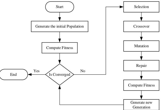
the algorithm finishes, the best solution returned. Genetic algorithms are particularly useful for problems where it is extremely difficult or impossible to get an exact answer, or for severe problems where a correct solution may not be required. They offer an exciting alternative to the typical algorithmic solution methods and are highly customizable. This notion can apply to a search problem. We consider a set of solutions for a challenge and select the set of best ones out of them. There are five phases considered in a genetic algorithm. In this study, we introduce a version of the Genetic Algorithm to solve the MOP model with both linear scalarization and compromise approaches. The flow of the proposed scheme displays in Figure 2.
Start
End
Generate the initial Population
Compute Fitness
Is Converged
Selection
Crossover
Mutation
Repair
Compute Fitness
Generate new Generation
Yes No
3.2. Genetic Algorithm Scheme
3.2.1. Genetic representation
Chromosome is represented as a matrix of 𝐺 rows and 𝑇 columns, rows 𝑖𝑡ℎ represent the section assignment for lecturer 𝑖𝑡ℎ. Cell (𝑔, 𝑡) contains section lecturer 𝑔𝑡ℎ assigned to at time-slot
𝑡𝑡ℎ, or 0 if lecturer 𝑔𝑡ℎ is not assigned to any section at time-slot 𝑡𝑡ℎ.
3.2.2. Fitness function
The fitness function contains two components: the penalty function and objective function. While the objective function focus on optimizing lecturer’s satisfaction, the penalty function deal with constraints. We separate constraints into 2 groups, group 1𝑠𝑡 includes constraint (𝐻4) handled by penalty function and group 2𝑛𝑑 includes the remaining constraints (𝐻1), (𝐻2), (𝐻3) handled by repair mechanism describe in section 3.2.4. So, we have the fitness function:
𝑓 = 𝑤𝑝𝑒𝑛∗ 𝑝𝑒𝑛 + 𝑤𝑜𝑏𝑗∗ 𝑜𝑏𝑗
Where 𝑝𝑒𝑛, 𝑜𝑏𝑗, 𝑤𝑝𝑒𝑛, 𝑤𝑜𝑏𝑗 are penalty function, objective function, penalty function weight and objective function weight respectively. Now, we have a lot of parameter that need decision maker to set, which makes it very difficult to find a good set of parameters. There is a way to solve that problem without changing the quality of the results is to normalize the penalty function, objective function and weights to 0-1 range. So we have the constraints: 0 ≤ 𝑤𝑝𝑒𝑛, 𝑤𝑜𝑏𝑗 ≤ 1 and 𝑤𝑝𝑒𝑛+ 𝑤𝑜𝑏𝑗 = 1.
Let 𝑉 be the number of lecturer violate constraint (𝐻4), the penalty function is normalized as follow:
𝑝𝑒𝑛 = 1
1 + 𝑉
The objective function depending on the approach is used will be normalized by different ways. The first appoach, linear scalarization:
𝑜𝑏𝑗1= ∑ (𝛼𝑔
∑𝐻ℎ=1𝑥ℎ,𝑔∗𝑎𝑠ℎ,𝑔
∑𝑆𝑆𝑠𝑠=1𝑥𝑠𝑠,𝑔∗max {𝑎𝑠,𝑔∣𝑠=1…𝑆}+ 𝛽𝑔
∑𝐻ℎ=1𝑥ℎ,𝑔∗𝑏𝑡ℎ,𝑔
∑𝑆𝑆𝑠𝑠=1𝑥𝑠𝑠,𝑔∗max {𝑏𝑡,𝑔∣𝑡=1…𝑇}+ 𝛾𝑔
1
1+|∑𝐻ℎ=1𝑥ℎ,𝑔−𝐷𝑔|+ 𝐺
𝑔=1
𝛿𝑔𝑝𝑜𝑑(∑ 𝑥ℎ,𝑔
𝐻
ℎ )
100 )
With constraints 0 ≤ 𝛼𝑔, 𝛽𝑔, 𝛾𝑔, 𝛿𝑔≤ 1 and 𝛼𝑔+ 𝛽𝑔+ 𝛾𝑔+ 𝛿𝑔= 1.
And the second approach, compromise programming:
𝑜𝑏𝑗2= 1 −
𝑑𝑖𝑠𝑡𝑎𝑛𝑐𝑒([𝐸1, 𝐸2, … , 𝐸𝐺], [𝐹1, 𝐹2, … , 𝐹𝐺])
𝑑𝑖𝑠𝑡𝑎𝑛𝑐𝑒([𝐸1, 𝐸2, … , 𝐸𝐺], [𝑄1, 𝑄2, … , 𝑄𝐺])
= 1 − √∑ ∑ (𝐸𝑖,𝑗− 𝐹𝑖,𝑗)
2 𝑇+1
𝑗=1 𝐺 𝑖=1
∑𝐺𝑖=1∑𝑇+1𝑗=1(𝐸𝑖,𝑗− 𝑄𝑖,𝑗)2
With 𝑄 is the matrix of the worse possible solution. 𝑄 ∈ ℝ𝐺×(𝑇+1)= {𝑄
1, 𝑄2, … , 𝑄𝐺} where 𝑄𝑔=
{𝑄𝑔,1, 𝑄𝑔,2, … , 𝑄𝑔,𝑇, 𝑄𝑔,𝑇+1, 𝑄𝑔,𝑇+2} is the vector of the worse timetable for lecturer 𝑔𝑡ℎ, such that:
𝑄𝑔,𝑗=
{
{0 𝑖𝑓 𝑠𝑠=1..𝑆𝑆∣𝑡𝑚max𝑠𝑠=𝑗 (𝑎𝑠𝑏𝑠𝑠,𝑔∗ 𝑏𝑗,𝑔) ∗ 2 > max_𝑟𝑎𝑡𝑖𝑛𝑔
max_𝑟𝑎𝑡𝑖𝑛𝑔 𝑂𝑡ℎ𝑒𝑟𝑤𝑖𝑠𝑒 𝑖𝑓 𝑗 ≤ 𝑇
{0 𝑖𝑓 𝐷𝑔∗ 2 > 𝑇
𝑇2 𝑂𝑡ℎ𝑒𝑟𝑤𝑖𝑠𝑒 𝑖𝑓 𝑗 = 𝑇 + 1
0 𝑜𝑡ℎ𝑒𝑟𝑤𝑖𝑠𝑒
Genetic operations
Denote:
• 𝑈 represents the size of the population.
• 𝑝𝑖𝑒 as the individual ith of the population at generation 𝑒𝑡ℎ, represented as chromosome matrix described in section 3.2.1. 𝑝𝑖𝑒𝑛,𝑚 denote the value of the cell at row 𝑛𝑡ℎ and column 𝑚𝑡ℎ.
• 𝜕𝑡 as the set of sections that learn at time-slot 𝑡𝑡ℎ.
• 𝜑 as the tournament size for selection.
• Β as the mutation rate
1. Generate the initial population: Columns 𝑘𝑡ℎ of an individual 𝑝
𝑖𝑒 contain 𝜕𝑘 and exactly
𝐺 − |𝜕𝑘| number 0. So, for each column 𝑘 ∣ 𝑘 = 1 … 𝑇, fill 𝜕𝑘 and 𝐺 − |𝜕𝑘| number 0 to
that column, and shuffle its element to ensure the randomness of the initialized population. After filling all column to chromosome matrix, apply repair operator to ensure the created chromosome respects constraints (𝐻1), (𝐻2), and (𝐻3).
2. Selection: we implemented the selection process based on Tournament Selection [32]. randomly select 𝜑 individuals from 𝑃𝑒 and perform a tournament that return the best individuals base on fitness value amongst them.
3. Crossover: Denote 𝑝𝑓𝑎𝑡ℎ𝑒𝑟𝑒 and 𝑝𝑚𝑜𝑡ℎ𝑒𝑟𝑒 are parents to crossover. The set of numbers in each column of 𝑝𝑓𝑎𝑡ℎ𝑒𝑟𝑒 and 𝑝𝑚𝑜𝑡ℎ𝑒𝑟𝑒 is permutation of each other, so we can choose any Ordered Crossover method to apply. Partially-mapped crossover (PMX) [33] is one of the most effective crossover technique for ordered list, so it is chosen in this study.
4. Mutation: For each individual 𝑝𝑖𝑒, have rate 𝐵 to swap only once for any 2 elements in any column. Similar to generating initial population process, the created chromosome after performing crossover and mutation must be applied repair operator to ensure there are no invalid results during the processing.
3.2.3. Repair Process
Input a chromosome matrix 𝑝 which may violate constraints (𝐻1), (𝐻2) and (𝐻3), genetic repair operator rearrange elements in 𝑝 so that new chromosome 𝑝′ satisfy all these constraints. Moreover, 𝑝′ should retain as many 𝑝’s genes as possible.
The purpose we combine constraints (𝐻1), (𝐻2), (𝐻3) into one group is because it’s very easy to convert them into the maximum matching problem in bipartite graph. In this study, we use Hopcroft-Karp algorithm [34], a polynomial algorithm to find the maximum matching.
The repair process is performed in 3 steps as follows:
1. Build a graph 𝒢 = (𝒱, ℰ), with vertex set 𝒱 = 𝒳 ∪ 𝒴, 𝒳 represents vertex set of 𝐺 × 𝑇
items for each lecturer in each timeslot, 𝒴 represents vertex set of 𝐻 items represent for sections. For each vertex ℊ𝓉 ∈ 𝒳 (ℊ𝓉 is the vertex represents for lecturer ℊ𝑡ℎ at timeslot
𝑡𝑡ℎ), ℎ ∈ 𝒴 (ℎ is the vertex represents for section ℎ𝑡ℎ), we add an edge from ℊ𝓉 to ℎ if
and only if 𝑡 = 𝑡ℎ, 𝑎𝑠ℎ,𝑔> 0 and 𝑏𝑡,𝑔> 0.
2. For each lecturer 𝑔 ∣ 𝑔 = 1 … 𝐺 at each timeslot 𝑡 ∣ 𝑡 = 1 … 𝑇, pair the vertex 𝑢 ∈ 𝒳 (u is the vertex represents for lecturer 𝑔𝑡ℎ at timeslot 𝑡𝑡ℎ) to vertex 𝑣 ∈ 𝒴 (𝑣 is the vertex represents for section 𝑝𝑔,𝑡 𝑡ℎ ) if 𝑝𝑔,𝑡> 0 and the pairing does not violate any constraints in
(𝐻1), (𝐻2), (𝐻3). This step aim to retain the good genes from 𝑝.
4. Experiment and Result
To evaluate the proposed model and algorithm, we use the data obtained in the spring semester of 2020 of the Computing Fundamental department at FPT University. A total of 𝐻 = 139 sections
of 𝑆 = 17 subjects assigned to 𝐺 = 27 lecturers. We built a webpage to collect lecturer preferences
of the subjects, time-slots and the number time-slots they want to teach, as shown in figure 3. The preferences received the values in range of 𝑎𝑠,𝑔 ∈ [0 … 5] and 𝑏𝑡,𝑔∈ [0 … 5]. All experiments mentioned in this report use a computer configured as follows: Processor: Intel(R) Xeon(R) CPU X5650 @2.67GHz (4 CPUs), ~2.3GHz; Memory: 8096MB RAM; all code implemented in java 8.
Figure 3: webpage to collect the preferences of a particular lecturer on the subjects and time-slots
The 𝑝𝑜𝑑 function is defined as:
Function: 𝑝𝑜𝑑
Input: {𝑥ℎ,𝑔| ℎ = 1. . 𝐻}
1: ℶ = 100
2: 𝑟=𝑁𝑢𝑚𝑃𝑜𝑑({𝑥ℎ,𝑔| ℎ = 1. . 𝐻})
3:
𝑛 = ∑ 𝑥ℎ,𝑔
𝐻
ℎ=1
4: If (1 ≤ 𝑛 ≤ 3) and (𝑟 = 1) Return ℶ
5: If (1 ≤ 𝑛 ≤ 3) and (𝑟 = 2) Return ℶ/5
6: If (1 ≤ 𝑛 ≤ 3) and (𝑟 ≥ 3) Return 0
7: If (4 ≤ 𝑛 ≤ 6) and (𝑟 = 2) Return ℶ
8: If (4 ≤ 𝑛 ≤ 6) and (𝑟 = 3) Return ℶ/5
10: If (1 ≤ 𝑛 ≤ 3) and (𝑟 = 1) Return ℶ
11: If (7 ≤ 𝑛 ≤ 8) and (𝑟 = 3) Return ℶ
12: If (7 ≤ 𝑛 ≤ 8) and (𝑟 = 4) Return ℶ/2
13: If (9 ≤ 𝑛 ≤ 10) Return ℶ
The 𝑁𝑢𝑚𝑃𝑜𝑑 function defined as:
Function: 𝑁𝑢𝑚𝑃𝑜𝑑 Input: {𝑥ℎ,𝑔| ℎ = 1. . 𝐻}
1: 𝑁𝑢𝑚 = 0
2: If (∑𝑡ℎ∈{𝑀1,𝑀2,𝑀3}𝑥ℎ,𝑔≥ 1) Then 𝑁𝑢𝑚 = 𝑁𝑢𝑚 + 1 3: If (∑𝑡ℎ∈{𝐸1,𝐸2,𝐸3}𝑥ℎ,𝑔≥ 1) Then 𝑁𝑢𝑚 = 𝑁𝑢𝑚 + 1 4: If (∑𝑡ℎ∈{𝑀4,𝑀5}𝑥ℎ,𝑔≥ 1) Then 𝑁𝑢𝑚 = 𝑁𝑢𝑚 + 1 5: If (∑𝑡ℎ∈{𝐸4,𝐸5}𝑥ℎ,𝑔≥ 1) Then 𝑁𝑢𝑚 = 𝑁𝑢𝑚 + 1 6: Return 𝑁𝑢𝑚
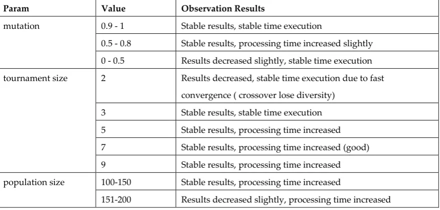
Genetic algorithms operate based on several parameters. They have a significant influence on the results of the algorithm. In this section, we describe how the values of this parameter are selected. To select the most suitable set of parameters for the genetic algorithm, we execute the algorithm multiple times. Observed effects to corresponding MOP approaches listed in Table 2 and Table 3.
Table 2: The observation result of the algorithm for each set of parameters with Scalarizing-objective function.
Param Value Observation Results
mutation 0.9 - 1 Stable results, stable time execution
0.5 - 0.8 Stable results, processing time increased slightly
0 - 0.5 Results decreased slightly, stable time execution
tournament size 2 Results decreased, stable time execution due to fast
convergence ( crossover lose diversity)
3 Stable results, stable time execution
5 Stable results, processing time increased
7 Stable results, processing time increased (good)
9 Stable results, processing time increased
population size 100-150 Stable results, processing time increased
151-200 Results decreased slightly, processing time increased
Table 3: The observation result of the algorithm for each set of parameters with Compromise-objective function.
Param Value Observation Results
mutation 0.9 - 1 Stable results, processing time increased slightly
0.5 - 0.8 Stable results, processing time increased
0 - 0.5 Stable results, stable time execution
tournament size 2 Results decreased slightly, stable time execution
3 Stable results, processing time increased
5 Stable results, stable time execution
7 Stable results, processing time decreased
9 Stable results, processing time decreased
151-200 Stable results decreased, processing time increased
For both approaches, the change of mutation rate value does not affect the convergence result and processing time of the algorithm. The tested ranges of the values of the parameters show good results. The small tournament size makes the crossover lose diversity. It negatively affects the algorithm results as well as the time of convergence. The tournament size = 7 seems to generate good results for the scalarizing approach, and tournament size > 9 increases processing time even though it maintains good fitness value. Population size > 100 gets worse for both fitness values and processing time. Based on the observed results, we selected the parameter set to run the algorithm according to Table 4.
Table 4: Parameters to run the algorithm corresponding to approaches
Param Approach
𝐵 𝑈 𝜑 Stop after 𝑤𝑜𝑏𝑗 𝑤𝑝𝑒𝑛
Scalarizing 0.9 100 7 30 0.3 0.7
Compromise 0.4 100 7 30 0.3 0.7
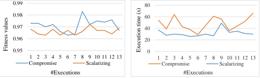
To evaluate the proposed algorithm with each fitness function. We have run the algorithm multiple times with the same initial value. Figures 4 shows the fitness values (objective values) of the Scalarizing and Compromise approaches. Both methods show that they are nearing expected values (approximately 1) on tested data. Although, it is not reasonable to compare value pairs of each technique at a particular execution. It noticed that Compromise shows fitness values slightly better when its achievement gets closer to 1 in all 13 runs. However, compromise programming shows that its execution time is slower average of 20 seconds in all executions. The fitness values’ change during
each generation of the Genetic Algorithm shown in Figure 6. We can see that the Compromise converges more slowly than Scalarizing. After about the first 20 generations, the fitness value has come very close to the convergence value. The reason for slower Compromise convergence may be that the mutation rate initially set to be lower than Scalarizing (0.4 versus 0.7).
Figure 4: Fitness values of two approaches over
several executions.
Figure 5: Execution time of the approaches over several executions.
The proposed model allows
to faculty preferences for both professional and time needs. It considers more aspects of the needs
of stakeholders than the simple ‘sum of favorites on the particular wish of lecturers’ model
introduced by previous researches [17] [21]. We use both preference and non-preference approaches for the multi-objective problem; meanwhile, most previous studies use the Scalarizing. It gives our users to have more options in the decision-making process. The decision-maker can thoroughly select Scalarizing to set weight for each instructor, in case he/she determines priority. Compromise programming gives a satisfactory answer in cases where there is not any priority assigned. Satisfaction level of each lecturer obtained by executing GA for compromise programming, shown in figure 7. It observed that teachers who are registered to teach many subjects, can teach in many
0.95 0.96 0.97 0.98 0.99
1 2 3 4 5 6 7 8 9 10 11 12 13
Fit
n
ess
v
alu
es
#Executions
Compromise Scalarizing
0 20 40 60 80
1 2 3 4 5 6 7 8 9 10 11 12 13
E
x
ec
u
tio
n
tim
e
(s
)
#Executions
different time frames and teach many various topics naturally prioritized. Meanwhile, with the current scoring of the target function: 100% ~ 5 stars of subjects * 5 stars of time slots, which leads to those who can teach few items, or have a lot of time constraints may receive a less-satisfied schedule. Scalarizing approach can provide "Artificial priority" through changing the parameters 𝛼𝑔, 𝛽𝑔, 𝛾𝑔, 𝛿𝑔.
Figure 6: Fitness values changing over generations for both scalarizing and compromise.
Figure 7: Satisfaction degrees of different lecturers generated by GA with compromise programming.
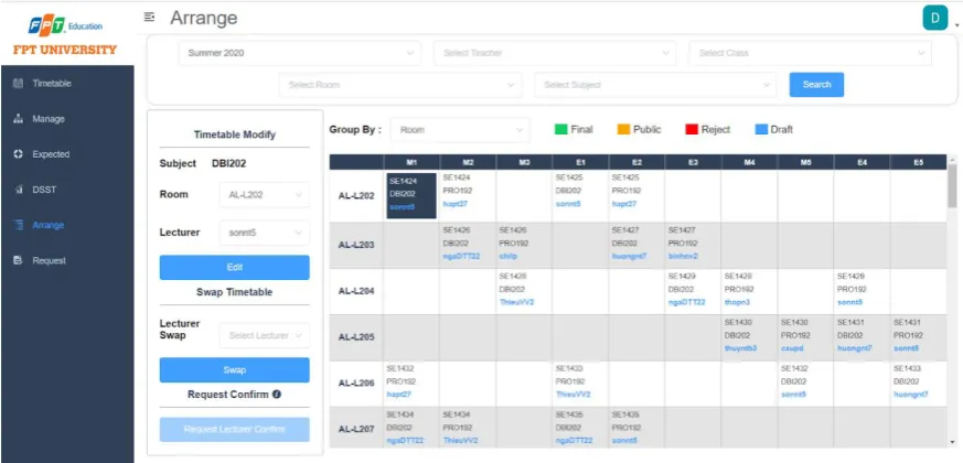
The Genetic Algorithm (and also other approximation algorithms) does not guarantee to find the global solution. The obtained solutions may be local optima. Decision-maker may have their customization on the provided schedule in this situation. To support them, modify the plan quickly, we design a web page to help drag and drop as shown in Figure 8. The decision-maker can choose any course and assign it to another instructor by dropping the item in the corresponding line. The information systems part plays a vital role in compensating for the shortcomings of the proposed algorithm.
Figure 8: The webpage allows the decision-maker to customize the generated schedule.
5. Conclusion
In this study, we have proposed a multi-objective optimization model for the assignment task. The proposed model satisfies the lecturers' preferences in terms of skills, time, and the number of jobs while ensuring related constraints. Our model is not only applicable to the FPT University lecturers scheduling problem but also defined a generic solution for multi-objective task assignment problems. We use two approaches, scalarizing and compromise programming, to turn the multi-objective problem into a single-multi-objective problem. Each method suits a different type of user. For the linear scalarizing approach, users can set different values for each weight of the target function. It is
0.55 0.6 0.65 0.7 0.75 0.8 0.85 0.9 0.95
F
it
ne
ss value
#Generations
Scalarizing Compromise0 0.2 0.4 0.6 0.8 1
1 3 5 7 9 11 13 15 17 19 21 23 25 27
Satis
fac
tio
n
Deg
ree
flexible, but in a multi-dimensional space, the visualization of the results corresponding to a parameter set is difficult. It leads to decision-makers to explore parameter sets in an ample search space. On the other hand, a compromise model is a single-shot solution for decision-makers. It avoids them having to define preference information for the objectives. The model itself has found a way to the best. However, the low use of parameters reduces the ability to interact with the model of a decision-maker. The proposed scheme for genetic algorithm shows that it works effectively; the repair step has removed all binding violation solutions without affecting the diversity of crossovers. Shortly, we are looking to build an integrated model with the scheduling of lecturers and students at the same time. Refining the parameters of the algorithm is also a job in our plan.
Funding: This research was funded by FPT University, grant number DHFPT/2020/12. The APC was funded by FPT University.
References
1. Andrade, P. R. L., Steiner, M. T. A., & Góes, A. R. T. (2019). Optimization in timetabling in schools using a mathematical model, local search and Iterated Local Search procedures. Gestão & Produção, 26(4), e3421. https://doi.org/10.1590/0104-530X3241-19.
2. Lemos, A., Melo, F. S., Monteiro, P. T., & Lynce, I. (2018). Room usage optimization in timetabling: A case study at Universidade de Lisboa. Operations Research Perspectives, 100092. doi: 10.1016/j.orp.2018.100092.
3. Ghiani, G., Manni, E., & Romano, A. (2017). Training offer selection and course timetabling for remedial education. Computers & Industrial Engineering, 111, 282–288. doi: 10.1016/j.cie.2017.07.034. 4. Vermuyten H, Lemmens S, Marques I, Beliën J. Developing compact course timetables with optimized
student flows. Eur J Oper Res 2016;251(2):651–61. https://doi.org/10.1016/j.ejor.2015.11.028.
5. Babaei, H., Karimpour, J., & Hadidi, A. (2015). A survey of approaches for university course timetabling problem. Computers & Industrial Engineering, 86, 43–59. doi: 10.1016/j.cie.2014.11.010. 6. D. W. Pentico, “Assignment problems: A golden anniversary survey, “European Journal of
Operational Research, vol. 176, no. 2, pp. 774–793, January 2007.
7. Daskalaki S., Birbas T., and Housos E. (2004) An integer programming formulation for a case study in university timetabling. European Journal of Operational Research, vol. 153, issue 1, pp. 117-135. 8. Yang, S., & Jat, S. N. (2011). Genetic algorithms with guided and local search strategies for university
course timetabling. Systems, Man, and Cybernetics, Part C: Applications and Reviews, IEEE Transactions on, 41 , 93–106.
9. Hmer, A., & Mouhoub, M. (2010). Teaching Assignment Problem Solver. Lecture Notes in Computer Science, 298–307. doi:10.1007/978-3-642-13025-0_32.
10. H. W. Kuhn, “The Hungarian method for the assignment problem,” Naval Research Logistics Quarterly, vol. 2, pp. 83–97, 1955.
11. M. L. Fisher, R. Jaikumar, and L. N. V. Wassenhove, “A multiplier adjustment method for the generalized assignment problem,” Management Science, vol. 32, no. 9, pp. 1095–1103, September 1986. 12. Lewis R. (2007) A survey of metaheuristic-based techniques for University Timetabling problems. OR
Spectrum, vol. 30, issue 1, pp. 167-190.
13. Muthuraman, S., & Venkatesan, V. P. (2017). A Comprehensive Study on Hybrid Meta-Heuristic Approaches Used for Solving Combinatorial Optimization Problems. 2017 World.
14. B. Sigl, M. Golub and V. Mornar, "Solving timetable scheduling problem using genetic algorithms," Proceedings of the 25th International Conference on Information Technology Interfaces, 2003. ITI 2003., Cavtat, Croatia, 2003, pp. 519-524.
15. A. Savić, D. Tošić, M. Marić, and J. Kratica, “Genetic algorithm approach for solving the task assignment problem,” Serdica Journal of Computing, vol. 2, pp. 267–276, 2008.
16. V. Sapru, K. Reddy and B. Sivaselvan, "Time table scheduling using Genetic Algorithms employing guided mutation," 2010 IEEE International Conference on Computational Intelligence and Computing Research, Coimbatore, 2010, pp. 1-4.
18. Corne D, Ross P, Fang H (1995) Evolving timetables. In: Lance C. Chambers (ed) The practical handbook of genetic algorithms, vol 1. CRC, Florida, pp 219–276.
19. Nouri, H. E., & Driss, O. B. (2016). MATP: A Multi-agent Model for the University Timetabling Problem. Software Engineering Perspectives and Application in Intelligent Systems, 11–22. doi:10.1007/978-3-319-33622-0_2.
20. Nouri, H. E., & Driss, O. B. (2013). Distributed model for university course timetabling problem. 2013 International Conference on Computer Applications Technology (ICCAT). doi:10.1109/iccat.2013.6521990.
21. Malik, B. B., & Nordin, S. Z. (2018). Mathematical model for timetabling problem in maximizing the preference level. doi:10.1063/1.5041568.
22. Santos HG, Uchoa E, Ochi LS, Maculan N. Strong bounds with cut and column generation for class-teacher timetabling. Ann Oper Res 2012;194(1):399–412. https://doi.org/10. 1007/s10479-010-0709-y. 23. Dorneles Á P, de Araújo OCB, Buriol LS. A fix-and-optimize heuristic for the high school timetabling
problem. Comput Oper Res 2014;52:29–38. https://doi.org/10.1016/j.cor.2014.06.023.
24. David A. Van Veldhuizen , Gary B. Lamont, “Multiobjective Evolutionary Algorithms: Analyzing the State-of-the-Art” (2000), DOI: 10.1162/106365600568158.
25. Ching-Lai Hwang; Abu Syed Md Masud (1979). Multiple objective decision making, methods and applications: a state-of-the-art survey. Springer-Verlag. ISBN 978-0-387-09111-2.
26. De Weck, O., & Kim, I. Y. (2004). Adaptive Weighted Sum Method for Bi-objective Optimization. 45th AIAA/ASME/ASCE/AHS/ASC Structures, Structural Dynamics & Materials Conference. doi:10.2514/6.2004-1680.
27. Zeleny, M. (1973), "Compromise Programming", in Cochrane, J.L.; Zeleny, M. (eds.), Multiple Criteria Decision Making, University of South Carolina Press, Columbia, pp. 262–301.
28. Ngo Tung Son, Le Van Thanh, Tran Binh Duong, and Bui Ngoc Anh. 2018. A decision support tool for cross-functional team selection: case study in ACM-ICPC team selection. In Proceedings of the 2018 International Conference on Information Management & Management Science (IMMS '18). ACM, New York, NY, USA, 133-138. DOI: https://doi.org/10.1145/3277139.3277149.
29. Ngo Tung Son, Tran Thi Thuy, Bui Ngoc Anh, and Tran Van Dinh. 2019. DCA-Based Algorithm for Cross-Functional Team Selection. In Proceedings of the 2019 8th International Conference on Software and Computer Applications (ICSCA '19). ACM, New York, NY, USA, 125-129. DOI: https://doi.org/10.1145/3316615.3316645.
30. Ngo, T.S.; Bui, N.A.; Tran, T.T.; Le, P.C.; Bui, D.C.; Nguyen, T.D.; Phan, L.D.; Kieu, Q.T.; Nguyen, B.S.; Tran, S.N. Some Algorithms to Solve a Bi-Objectives Problem for Team Selection. Appl. Sci. 2020, 10, 2700.
31. S. M. Thede, “An Introduction to Genetic Algorithms,” Journal of Computing Sciences in Colleges, vol. 20, no. 1, pp. 1–1, 2004.
32. Miller, Brad; Goldberg, David (1995). "Genetic Algorithms, Tournament Selection, and the Effects of Noise" (PDF). Complex Systems. 9: 193–212.
33. Otman, A., & Jaafar,A. (2011). A comparative study of adaptive crossover operators for genetic algorithms to resolve the travelling salesman problem. International Journal of Computer Applications, 31(11), 49-57.