https://doi.org/10.1007/s11128-018-2107-3
Time–space complexity of quantum search algorithms in
symmetric cryptanalysis: applying to AES and SHA-2
Panjin Kim1·Daewan Han1·Kyung Chul Jeong1
Received: 30 July 2018 / Accepted: 22 October 2018 © The Author(s) 2018
Abstract
Performance of cryptanalytic quantum search algorithms is mainly inferred fromquery complexity which hides overhead induced by an implementation. To shed light on quantitative complexity analysis removing hidden factors, we provide a framework for estimating time–space complexity, with carefully accounting for characteristics of target cryptographic functions. Processor and circuit parallelization methods are taken into account, resulting in the time–space trade-off curves in terms ofdepthandqubit. The method guides how to rank different circuit designs in order of their efficiency. The framework is applied to representative cryptosystems NIST referred to as a guideline for security parameters, reassessing the security strengths of AES and SHA-2.
Keywords Quantum circuit·Grover·Parallelization·Resource estimates·AES·
SHA-2
Mathematics Subject Classification 94A60·68Q12·81P68
1 Introduction
Quantum cryptanalysis is an area of study that has long been developed alongside the field of quantum computing, as many cryptosystems are expected to be directly affected by quantum algorithms. It is thus natural that cryptographic communities are putting more and more efforts for preparing post-quantum era as quantum computing communities are making progress. A notable effort being made by National Institute of Standards and Technology (NIST) primarily concerns new public-key cryptosystems leveraged by the quantum period-finding algorithm that might make some currently used public-key schemes obsolete once a practical quantum computer becomes avail-able [1]. Unlike public-key schemes, however, the significance of quantum search
B
Kyung Chul Jeong [email protected]algorithms in symmetric cryptosystems is arguable. It had been widely known that most symmetric cryptosystem’s security levels will be simply reduced by half due to the asymptotic behavior of the query complexity of Grover’s algorithm under the ora-cle assumption [2]. Square-root improvement in exhaustive-search ability seems on the one hand not negligible and may affect the current symmetric cryptosystems like in key sizes. On the other hand, when the detailed mechanism ‘how quantum objects or Grover’s speedup work’ comes into account, there exist claims that the threat is not as harmful as it has been believed to be [1,3].1The main reason for devaluating the algorithm in symmetric cryptography stems from its ‘poor parallelizability.’
As the field has matured over decades, not mere asymptotic but more quantitative approaches to the cryptanalysis are also being considered recently [4–9]. These works have substantially improved the understanding of quantum attacks by systematically estimating quantum resources. Nevertheless, it is still noticeable that the existing works on resource estimates are more intended for suggesting exemplary quantum circuits (so that one can count the number of required gates and qubits explicitly) than fine-tuning of actual attack designs. Furthermore, despite that the parallelizability of quantum search algorithms is the main source of the debate on the quantum threat in symmetric cryptography, the resource cost of parallel quantum attack has never been estimated quantitatively. In fact, quantum search algorithms have never been applied to parallel applications in gate-level details, not just in quantum cryptanalysis but in the whole field of quantum information. There could be various difficulties hampering the parallelizing quantum algorithms, just as many classical serial applications cannot find its parallel counterparts easily.
The importance of estimating costs of quantum search algorithms beyond pioneer-ing works should be emphasized as it can be utilized to suggest practical security levels in the post-quantum era. NIST indeed suggested security levels based on the resistances of advanced encryption standard (AES) and secure hash algorithm (SHA) to quantum attacks in PQC standardization call for proposals document [10]. In addi-tion, the difficulty of measuring the complexity of quantum attacks was questioned in the first NIST PQC standardization workshop.2The main purpose of this work is to formulate the time–space complexity of quantum search algorithms in order to provide reliable quantum security strengths of classical symmetric cryptosystems.
1.1 This work
There exist two noteworthy points overlooked in the previous works. First, the target function to be inverted is generally a pseudo-random function or a cryptographic hash function. Under the characteristics of such functions, bijective correspondence between input and output is not guaranteed. This makes Grover’s algorithmseemingly inapplicable due to the unpredictability of the number of targets. The second point is a time–space trade-off of quantum resources. Earlier works on quantitative resource
1 See also ‘S. Fluhrer, Reassessing Grover’s algorithm,http://eprint.iacr.org/2017/811,’ which analyzed
parallelizability of Grover’s algorithm in conjunction with cryptosystems.
2 Interested readers are suggested to look into ‘Moody, D.: Let’s get ready to rumble—the NIST PQC
estimates have implicitly or explicitly assumed a single quantum processor. Presuming that theresourcein classical estimates includes the number of processors the adversary is equipped with, the single processor assumption is something that should be revised. Being aware of the issues, we come up with a framework for analyzing the time– space complexity of cryptanalytic quantum search algorithms. The main consequences we present in this paper are threefolded:
1.1.1 Precise query complexity involving parallelization
The number of oracle queries, or equivalently Grover iterations, is first estimated as exactly as possible, reasonably accounting for previously overlooked points. Random statistics of the target function are carefully handled which lead to increase in iteration number compared with the case of a unique target. Surprisingly, however, the cost of dealing with random statistics in this paper is not expensive compared with the previous work [6] under the single processor assumption. Furthermore, when processor parallelization is considered, we observed that this extra cost gets even more negligible. It is also interesting to recognize that the parallelization methods could vary depending on the search problems. After taking the asymptotical big O notation off, the relation between time and space in terms of Grover iterations and number of processors, called trade-off curve, is obtained. Apart from resource estimates, investigating the trade-off curve of state-of-the-art collision finding algorithm in [11] with optimized parameters is one of our major concerns.
1.1.2 Depth-qubit trade-off and circuit design tuning
In the next stage, time and space resources are defined in a way that they can be inter-preted as physical quantities. Cost of quantum circuits for cryptanalytic algorithms can be estimated in units ofToffoli-depthsandlogical qubits. Taking the total num-ber of gates as time complexity disturbs accurate estimates for the speed of quantum algorithms due to far different overheads introduced by various gates in real opera-tion. With the definitions of quantum resources, the trade-off curve now describes the relation between circuit depths and number of qubits. Since we are given a ‘relation’ between time and space, it is then possible to grade the various quantum circuits in order of efficiency. In other words, the method described so far enables one to tell which attack design is more cost-effective.
By applying generic methodology newly introduced, time–space complexities of AES and SHA-2 against quantum attacks are measured in the following way.3Various designs are constructed by assembling different circuit components with options such as reduced depth at the cost of the increase in qubits (or vice versa). Design candidates are then subjected to the trade-off relation for comparison. The trade-off coefficient of the most efficient design represents the hardness of quantum cryptanalysis. Compared with pre-existing circuit designs, we have improved the circuits by reducing required
3 We concluded that quantum cost of attacking SHA-3 is more expansive than that of SHA-2, based on [5]
264 296 2128 2160 2192 264
296
232 232
Level I
(AES-128)
Level III
(AES-192)
Level V
(AES-256)
Level IV
(SHA-384)
Level II
(SHA-256)
264 296 2128 2160 2192 264
296
232 232
Level I
(AES-128)
Space
Time
Level III
(AES-192)
Level V
(AES-256)
Level IV
(SHA-384)
Level II
(SHA-256)
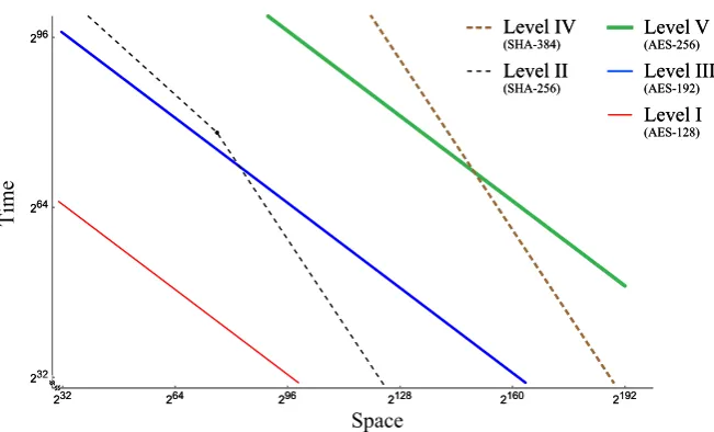
Fig. 1 Time–space cost, which has conditional ordering, of the quantum attacks on five security strength category representatives of NIST PQC standardization
qubits and/or depths in various ways. However, we do not claim that we have found the optimal attacks for AES and SHA-2. The method enables us to select the best one out of candidates at hand.
1.1.3 Revisiting the security levels of NIST PQC standardization
The procedure is applied to each primitive of security strength categories NIST spec-ified in [10]. A new threshold that is required for the category classification, based on the cost metric proposed in this work, is provided in Fig.1. It includes a wide range of parameters and the quantum collision finding algorithms which do not outperform classical counterparts to explicitly recognize the quantum-side complexities of all the categories.
We end this subsection with two important caveats. One is that a use of classical resources appears in this paper, but we do not handle the complexity induced by it because of unclear comparison criteria for quantum and classical resources. The other is that our focus is put on specific algorithms implemented in the level of elementary gates. Readers are however encouraged not to rule out other algorithms that quantum computing communities also pursuit, for example, ones using quantum memory.
1.2 Organization
time–space analysis to AES and SHA-2. In Sect.8, based on the observations made in the previous sections, a comprehensive figure summarizing the quantum security strengths of AES and SHA-2 is drawn. Section9summarizes the paper.
2 Backgrounds
Grover’s algorithm, the success probability, parallelization methods, and some gener-alizations or variants are explained briefly. A brief review of AES and SHA-2, and an introduction to related works on resource estimates are followed. We do not cover the basics of quantum computing, but leave the references [12,13] for interested readers. Throughout the paper, the target function is denoted by f,N =2nfor somen ∈N and every bra or ket state is normalized.
2.1 Grover’s algorithm
Consider a setXof sizeN and a function f: X → {0,1},
f(x)=
1, ifx∈T, 0, otherwise,
whereT of sizetis a set of targets to be found.
Grover’s algorithm [2] is an algorithm that repeatedly applies an operator
Q= −AS0A−1Sf,
calledGrover iteration, to the initial state| = A|0, where
A=H⊗n, S0=I−2|00|, Sf =I−2|ττ|, (1)
whereH⊗nis a set of Hadamard operators and|τis a target state which is an equal-phase and equal-weight superposition of|xfor allx∈T. The roles ofS0andSf are
to swap the sign of zero and|τstates, respectively.
The operators Sf and −AS0A−1 are known as oracleand diffusion operators,
respectively. By acting the oracle operator on a state, only the target state is marked through the sign change. The diffusion operator flips amplitudes around the average. Success probability of measurement as a function of the number of iterations has been studied in [14], observing the optimal number of iterations that minimizes the ratio of the iterations to success rate. We introduce the results below with notation that is used throughout the paper.
By applyingQon the initial statei-times, the success probability of measuring one of thet solutions, denoted bypt,N:Z≥0→ [0,1], becomes
pt,N(i)=sin2
(2i+1)·θt,N
where sinθt,N
=√t/N(= |τ). The number of repetitions ofQmaximizing the probability of measurement, denoted byItmp,N ∈N, is estimated as4
Itmp,N =π 4 ·
N
t . (3)
When the measurement is made afteri-repetitions of Q, the expected number of Grover iterations to find one of the targets can be expressed as a function ofi. Fort targets in the domain of size N, the function is denoted by It,N: N→ R>0 which
readsIt,N(i)=i/pt,N(i). The optimal number of iterationsit,N∈Nthat minimizes
It,Nis found to beit,N =0.583. . .·√N/t, and then the expected number of iterations,
denoted byIt,N ∈N, reads
It,N=It,N(it,N)=0.690. . .·
N
t . (4)
In some cases, the domain sizeN is omitted such as pt(i)(= pt,N(i))orIt(=It,N),
for readability.
2.2 Parallelization
Parallelization of Grover’s algorithm using multiple quantum computers has been investigated in applications to cryptanalysis [1,10,15]. Consideration of parallelization in a hybrid algorithm can be found in [16]. Asymptotically the execution time is reduced by a factor of the square root of the number of quantum computers. There are two straightforward parallelization methods having such property, calledinner and outerparallelization.
Parameters Tq andSq stand for the number of sequential Grover iterations and
the number of quantum computers, respectively.Scstands for the amount of classical
resources, such as the size of storage and/or the number of processors. Definitions of two parallelization methods can be given as follows.
Definition 1 [Inner Parallelization (IP)] After dividing the entire search space into
Sqdisjoint sets, each machine searches one of the sets for the target. The number of
iterations can be reduced due to the reduced domain size.
Definition 2 [Outer Parallelization (OP)] Copies of Grover’s algorithm on the entire
search space are run onSqmachines. Since it is successful if any of theSqmachines
finds the target, the number of iterations can be reduced.
Parallelization is inevitable once the notion of MAXDEPTH is considered [10]. MAXDEPTH is a parameter for a circuit depth that a quantum computer can run without errors. We do not cover the reasoning behind the notion, but suggest for interested readers to look into NIST’s PQC call for proposals document and related comments. Three MAXDEPTH parameters we adopt from [10] are as follows.
– 240: Approximate number of logical gates that presently envisioned quantum com-puting architectures are expected to serially perform in a year.
– 264: Approximate number of logical gates that current classical computing archi-tectures can perform serially in a decade.
– 296: Approximate number of logical gates that atomic scale qubits with speed of light propagation times could perform in a millennium.
2.3 Generalizations and variants
Fixed-point [17] and quantum amplitude amplification (QAA) [18] algorithms are generalizations of Grover’s algorithm. A brief review of QAA is given in this subsec-tion which appears as a component of a collision finding algorithm in later secsubsec-tions. We skip over the fixed-point algorithm as it has no advantage over Grover’s algorithm and QAA in this work.5
There exist a number of variants of Grover’s algorithm in application to collision finding. In [19], Brassard, Høyer, and Tapp suggested a quantum collision finding algorithm (BHT) of O(N1/3)query complexity usingquantum memoryamounting
to O(N1/3) classical data. A multi-collision algorithm using BHT was suggested in [20]. In this work however, we do not consider BHT as a candidate algorithm for the following reasons. One is that the algorithm entails a need for quantum memory where the realization and the usage cost are controversial [21], and the other is that we are unable to come up with any implementation restricted to use of elementary gates that do not exceed the total cost ofO(N1/2).
Apart from quantum circuits, algorithms primarily designed for other type of mod-els such as measurement-based quantum computation also exist, for example quantum walk search [22,23] or element distinctness [24], but we do not cover them as state-of-the-art quantum architecture is targeting for circuit computation. Interested readers may further refer to [20] and related references therein for more information on quan-tum collision finding.
Bernstein analyzed quantum and classical collision finding algorithms in [3]. Quot-ing the work, no quantum algorithm with better time–space product complexity than O(N1/2)which is achieved by the state-of-the-art classical algorithm [25] had not been
reported. If Grover’s algorithm is parallelized with the distinguished point method, complexity of O(N1/2)can be achieved. This is one of the examples ofimmediate waysto combine quantum search with the rho method as mentioned in [3]. We denote it as Grover with distinguished point (GwDP) algorithm in this paper.
In ASIACRYPT 2017, Chailloux, Naya-Plasencia, and Schrottenloher suggested a new quantum collision finding algorithm, called CNS algorithm, of O(N2/5)query complexity usingO(N1/5)classical memory [11].
5 There are two reasons. One is that fixed-point search requirestwooracle queries per iteration, and the
2.3.1 QAA algorithm
Basic structure of QAA is the same as Grover’s original algorithm. Initial state| = A|0 is prepared, and then Grover iteration Q is repeatedly applied i times to get success probability Eq.2. The only difference is that in QAA, the preparation operator Ais not restricted toH⊗nwhereN =2n, and so thus the search space can be arbitrarily defined. Detailed derivation is not covered here, but instead we describe the key feature in an example.
As a trivial example, let us assume we are given a quantum computer and try to find a target bit-string 110011 in a setN = {x | x ∈ {0,1}6 and two middle bits are 0}. Domain size is not equal to 26, and the initial state can be prepared byA=H
1H2H5H6
where Hr is Hadamard gate acting onr-th qubit. Remaining processes are to apply
Grover iterations Q = −AS0A−1Sf with Agiven by the state preparation operator
just mentioned. The search space examined is rather trivial, but QAA also works on arbitrary domain. Nontrivial domain can be given as something like N = {x | x ∈
{0,1}6, f(x) = 0}for some given function f. It is a matter of preparing a state encoding appropriate search space, or in other words, that is to find an operator A. OnceAis constructed, QAA works in the same way as in Grover’s algorithm.
2.3.2 GwDP algorithm
GwDP algorithm is a parallelization of Grover’s algorithm. Distinguished points (DP) can be defined by function outputs whosed most significant bits are zeros, denoted byd-bit DP. We allow the notation DP to indicate inputs to produce DP or pairs of DP and corresponding input.
ForSq = Sc = 2s, we use(n−2s)-bit DP. By runningTq = O
2n/2−stimes of Grover iterations, DP is expected to be found on each machine. Storing O(2s) DPs sorted according to the output, a collision is found with high probability. The time–space product is alwaysTqSq =O
N1/2.
2.3.3 CNS algorithm
Instead of the details of CNS algorithm [11], we briefly mention the high-level descrip-tion and the corresponding complexities.
CNS algorithm consists of two phases, the list preparation and the collision finding. In the list preparation phase, a list of size 2lofd-bit DPs is drawn up with the time com-plexity ofO(2l+d/2)and the classical storage of sizeO(2l). In the collision finding phase QAA algorithm is used. Each iteration of QAA algorithm consists ofO(2d/2) Grover iterations andO(2l)operations for the list comparison. After O2(n−d−l)/2 QAA iterations, a collision is expected to be found. In total, CNS algorithm has O2l+d/2+2(n−d−l)/2(2d/2+2l)time complexity and usesO(2l)classical mem-ory. With the optimal parameters l = d/2 and d = 2n/5, a collision is found in Tq =O(N2/5)withSc=O(N1/5).
IfSq =2s, time complexity becomesO(2(n−d−l−s)/2(2d/2+2l)+2l+d/2−s)for
s ≤min(l,n−d−l). Whenl =d/2 andd =2/5{n+s}, the complexities satisfy
2.4 AES and SHA-2 algorithms
A brief review of AES and SHA-2 is given in this subsection. Specifically, AES-128 and SHA-256 algorithms are described which will form the main body of later sections.
2.4.1 AES-128
Only the encryption procedure of AES-128 which is relevant to this work will be shortly reviewed. See [26] for details.
Round AES round consists of four elementary operations: SubBytes, ShiftRows, MixColumns, and AddRoundKey.6 Each operation applies to internal state, which is represented by 4×4 array of bytesSi,j, as shown in Fig.2a.
– ShiftRows does cyclic shifts of the last three rows of the internal state by different offsets.
– MixColumns does a linear transformation on each column of the internal state that mixes the data.
– AddRoundKey does an addition of the internal state and the round key by an XOR operation.
– SubBytes does a nonlinear transformation on each byte. SubBytes works as substitution-boxes (S-box) generated by computing a multiplicative inverse, fol-lowed by a linear transformation and an addition of S-box constant.
Key ScheduleAES key schedule consists of four operations: RotWord, SubWord, Rcon, and addition by XOR operation. The sequence of key scheduling is described in Fig.2b. Each operation applies to 32-bit wordwi, which is represented by 4×1 array of bytes
kid,j. First four words are given by original key which become the zeroth round key. More words—40 in AES-128—are then generated by recursively processing previous words. Every sixteen-bytekid,j constitutesd-th round key. RotWord, SubWord, and Rcon only apply to every fourth wordwi, i ∈ {3,7,11, . . .39}.
– RotWord does a cyclic shift on four bytes.
– Rcon does an addition of the constant and the word by XOR operation. – SubWord does an S-box operation on each byte in word.
2.4.2 SHA-256
For brevity, only SHA-256 hashing algorithm for one message block which is rele-vant to this work will be reviewed. Description of preprocessing including message padding, parsing, and setting initial hash value is also omitted here. See [27] for details.
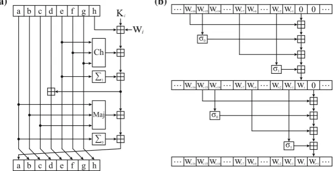
RoundSHA-2 round consists of five operations:Ch, Maj,0,1, and addition modulo
232. Round operations apply on eight 32-bit working variables denoted bya, b, c, d, e, f, g, h. See Fig.3a for procedures.
(a) (b) SubBytes ShiftRows MixColumns AddRoundKey
S
0,0S
1,0S
2,0S
3,0S
0,1S
1,1S
2,1S
3,1S
0,2S
1,2S
2,2S
3,2S
0,3S
1,3S
2,3S
3,3S
0,0’S
1,0’S
2,0’S
3,0’S
0,1’S
1,1’S
2,1’S
3,1’S
0,2’S
1,2’S
2,2’S
3,2’S
0,3’S
1,3’S
2,3’S
3,3’k
0,0 0k
1,0 0k
2,0 0k
3,0 0k
0,1 0k
1,1 0k
2,1 0k
3,1 0k
0,2 0k
1,2 0k
2,2 0k
3,2 0k
0,3 0k
1,3 0k
2,3 0k
3,3 0 Input Key RotWord SubWord Rconk
0,0 1k
1,0 1k
2,0 1k
3,0 1k
0,1 1k
1,1 1k
2,1 1k
3,1 1k
0,2 1k
1,2 1k
2,2 1k
3,2 1k
0,3 1k
1,3 1k
2,3 1k
3,3 1 RotWord SubWord Rconk
0,0 2k
1,0 2k
2,0 2k
3,0 2k
0,1 2k
1,1 2k
2,1 2k
3,1 2k
0,2 2k
1,2 2k
2,2 2k
3,2 2k
0,3 2k
1,3 2k
2,3 2k
3,3 2 … … … … 0 th 1 ye k d n u or st 2 ye k d n u or nd round keyw0 w1 w2 w3
w4 w5 w6 w7
w8 w9 w10 w11
Fig. 2 aRound operations andbkey schedule of AES-128 algorithm. Each square box accommodates one byte. In key schedule, 128-bit key is divided into four 32-bit words
(a) (b)
a b c d e f g h
a b c d e f g h Ch
w
i Ki ∑1 Maj ∑0…wi-16wi-15wi-14…wi-7wi-6…wi-2wi-1 0 0 …
σ0
σ1
…wi-16wi-15wi-14…wi-7wi-6…wi-2wi-1wi 0 …
σ0
σ1
…wi-16wi-15wi-14…wi-7wi-6…wi-2wi-1wi wi+1…
– C h(x,y,z)=(x∧y)⊕(¬x∧z),
– Ma j(x,y,z)=(x∧y)⊕(x∧z)⊕(y∧z), – 0(x)=R O TR2(x)⊕R O TR13(x)⊕R O TR22(x),
– 1(x)=R O TR6(x)⊕R O TR11(x)⊕R O TR25(x),
whereR O TRn(x)is circular right shift ofxbynpositions.
Message ScheduleSHA-2 message schedule consists of three operations:σ0,σ1, and
addition modulo 232. The sequence of message scheduling is described in Fig.3b. Each operation applies to 32-bit wordWi. First 16 words are given by original message
block which become the first 16 words fed to SHA-256 rounds. More words—48 in SHA-256—are then generated by recursively processing previous words.
– σ0(x)=R O TR7(x)⊕R O TR18(x)⊕SHR3(x),
– σ1(x)=R O TR17(x)⊕R O TR19(x)⊕SHR10(x),
whereSHRn(x)is right shift ofxbynpositions.
2.5 Quantum resource estimates
Quantum resource estimates of Shor’s period-finding algorithm have long been studied in the various literature. See for example [8,28] and referenced materials therein. On the other hand, quantitative quantum analysis on cryptographic schemes other than period finding is still in its early stage. Partial list may include attacks on multivariate-quadratic problems [9], hash functions [5,7], and AES [4,6]. We introduce two of them which are the most relevant to our work.
2.5.1 AES key search
Grassl et al. reported the quantum costs of AES-kkey search fork∈ {128,192,256} in the units of logical qubit and gate [6]. In estimating the time cost, the author’s focus was put on a specific gate called ‘T’ gate and its depth, although the overall gate count was also provided. Space cost was simply estimated as the total number of qubits required to run Grover’s algorithm.
2.5.2 SHA-2 and SHA-3 pre-image search
Amy et al. reported the quantum costs of SHA-2 and SHA-3 pre-image search in the units of logical and physical qubit and gate [5]. The method considers an error-correction scheme called surface code. Time cost was set considering the scheme. Estimating the costs of T gates in terms of physical resources was one of the main results. One point we would like to address in the work is that random-like behavior of SHA function was not considered. It is assumed in the paper that the unique pre-image of a given hash exists.
3 Trade-off in query complexity
In this section, the definitions of cryptographic search problems and the query-based time cost of the corresponding quantum search algorithms are discussed. The trade-off equations between the number of queries and the number of machines are given as a result.
3.1 Types of search problems
We assume that f: X → Y is a random function which means f is selected from the set of all functions fromXtoY uniformly at random. Useful statistics of random functions can be found in [29]. The probabilities related to the number of pre-images are quoted below. When an elementxis selected from a setX uniformly at random,
it is denoted byx←$ X.
When|Y| = Nand|X| =a N ∈Nfor somea∈Q, an elementy∈Yis called a j
-nodeif it has jpre-images, i.e.,|{x∈ X: f(x)=y}| = j. Fory←$ Y, the probability ofyto be a j-node, denoted byq(a N): Z≥0→ [0,1], is
q(a N)(j)≈
1 ea ·
aj
j!. (5)
Forx←$ X, the probability of f(x)to be a j-node, denoted byr(a N):N→ [0,1], is
r(a N)(j)≈ j·q(a N)(j). (6)
These approximations can hold whena N is larger than j. However, since the values are very small at large j, we may assume that Eqs. 5and6 are valid in the entire domain.
The formal definitions of search problems relevant to symmetric cryptanalysis can be described with random functions. The way of generating the given information in each problem is carefully distinguished. The first is Key Search generalized from the secret key search problem using a pair of plaintext and ciphertext of an encryption algorithm.
Definition 3 [Key Search (KS)] For a random function f: X → Y, y = f(x0)is
generated from anx0∈X.Key Searchis to findthetargetx0for given f andy.
The existence of the targetx0inX is always ensured. However, pre-images ofy
other thanx0 can be found, which is called afalse alarm. The false alarms have to
be resolved by additional information since no clue (that helps to recognize the real target) is given within the problem.
Definitions generalized from the pre-image and the collision problems of CHF are given as follows.
Definition 4 [Pre-image Search (PS)] For a random function f: {0,1}∗ → Y, yis
chosen at random,y←$Y, or equivalently, y= f(x0)for anx0 ∈ {0,1}∗.Pre-image
Searchis to findany x∈ {0,1}∗satisfying f(x)=yfor given f andy.
There is no false alarm in Pre-image Search. However, the existence of a pre-image in a fixed subset of{0,1}∗cannot be ensured.
Definition 5 [Collision Finding (CF)] For a given random function f: {0,1}∗→Y,
Collision Findingis to findanyinputsx1,x2∈ {0,1}∗satisfying f(x1)= f(x2).
3.2 Trade-off in Grover’s algorithm for Key Search
In this subsection, the expected iteration number and the parallelization trade-off of Grover’s algorithm are given. We assume that f: X →Y and|X| = |Y| =N.
In Key Search, the giveny∈Ybecomest-node with probabilityr(t)of Eq.6. The probability that one of the pre-images ofyis found by the measurement afteri-times Grover iterations becomes pt(i)of Eq.2. Since only one target amongt pre-images
is the true key, the probability that the answer is correct is 1/t. ForPrandKS:N→ [0,1], PrandKS(i)denotes the success probability after i-times Grover iterations of the Key Search. To emphasize that f is assumed to be a random function, the subscript ‘rand’ is specified.PrandKS(i)is the summation over possiblet’s,
PrandKS(i)=
t≥1
r(t)·pt(i)·
1
t. (7)
Proposition about the optimal expected iterations follows.
Proposition 1 The optimal expected number, IrandKS, of Grover iterations for Key Search
becomes
Proof This proof is similar to the one in Sect. 4 of [14].
If the measurement is taken afteri-times Grover iterations, the expected number of iterations can be expressed as a function ofi, denoted byIrandKS :N→R>0, which reads
IrandKS(i)=
i PrandKS(i).
The optimal value, IrandKS ∈ N, is approximated as the first positive local minimum value ofIrandKS(i). The integer closest to the first positive root of derivative ofIrandKS(i), denoted byirandKS ∈N, can be calculated by a numerical method. The result isirandKS =
0.434. . .·√N andIrandKS =IrandKS(irandKS).
ComparingIrandKS withI1of Eq.4, the expected iteration increases by 37.8…%.
The parallel trade-off curve of Key Search is calculated in the rest of this subsection. If inner parallelization method is taken forSq1, the number of pre-images ofyin
each divided space becomes only 0 or 1 for overwhelming probability, even though f is a random function. Therefore, the success probability afteri-times iterations, denoted byPrandKS:IP:N→ [0,1], reads
PrandKS:IP(i) = PrandKS:IP,N(i)
= p1,(N/Sq)(i), (8)
from Eq.2. The optimal expected iteration number is similar to Eq.4as
IrandKS:IP =I1,(N/Sq)=0.690. . .·
N/Sq
. (9)
In outer parallelization method, the success probability after i-times iterations becomes
PrandKS:OP(i)=1− 1−PrandKS(i)
Sq
,
and then the optimal expected iteration number forSq1 is given by
IrandKS:OP=0.784. . .·
(N/Sq). (10)
As a result, inner parallelization is 11.9. . .% more efficient than outer method in Key Search. We denote the number of machines used in Key SearchSqKS. The optimal expected number of iterations in Key Search, denoted byTqKS, can be considered as
IrandKS:IP.
Proposition 2 (KS trade-off curve) For SqKS 1, the parallelization trade-off of
Grover’s algorithm for Key Search is given by
TqKS
2
SqKS=0.476. . .·N.
3.3 Trade-off in Grover’s algorithm for Pre-image Search
Let X be the restricted domain of the function f: {0,1}∗ → Y, and assume|X| =
|Y| = N. We may assume that the restriction of f onX, denoted by f|X, is also a random function. In Pre-image Search, there existt pre-images of the giveny with probabilityq(t)in Eq.5. The success probability of measuring one of the targets after i-times iterations is a summation ofq(t)·pt(i)over possiblet’s as
PrandPS (i)=
t≥0
q(t)·pt(i).
Since p0(i)=0 andq(t)=r(t)/tfort≥1, it can be written asPrandPS (i)=PrandKS(i).
The important difference between Key Search and Pre-image Search is the existence of failure probability. If the domain of size N is used, the probability there is no pre-image ofyinX isq(0)=1/e≈0.368. . ..
Two resolutions can be sought. The first is to change the domainXin every execution of Grover’s algorithm. In this case, the result on the optimal iteration number of Pre-image Search becomes the same as Proposition1. The second is to expand the domain,
|X| =a N ∈ Nfor somea >1. The success probability then readsPrandPS,(a N)(i)=
t≥1q(a N)(t)·pt,(a N)(i).
Proposition 3 If|X| N , the optimal expected number of iterations, denoted by
IrandPS ,(N), for Pre-image Search is written as
IrandPS,(N)=0.690. . .·√N.
WhenN =2256, the proposition can be assumed to hold fora≥210. Subscript ‘1’ specifies the assumption. The fact thatIrandPS ,(N)≈I1,N, i.e., better performance up
to some converged value for larger domain size, is remarked. Ifa grows to 8, the failure probability decreases below 0.0004. . .≈1/e8.
In the case of inner parallelization for|X| = |Y|, the pre-images ofyare distributed to different divided spaces with overwhelming probability whenSq 1. The success
probability reads
PrandPS:IP,N(i)=
t≥1
q(t)·
1−1−p1,(N/Sq)(i) t
.
and the optimal expected iteration number is written as
IrandPS:IP,N =0.981. . .·
(N/Sq). (11)
SincePrandPS(i)=PrandKS(i), the behavior of outer parallelization of Pre-image Search is the same as in Key Search. The optimal expected iteration number is
IrandPS:OP=0.784. . .·
(N/Sq) =IrandKS:OP
When|X| = a N ∈ Nfor some a > 1, if Sq > a2, it can be assumed that all
pre-images ofyare separately distributed to the divided space in inner parallelization. For both of inner and outer parallelization, the optimal expected iteration converges to the value of Eq.12whena 1 andSq>a2.
There are subtleties in comparing inner and outer parallelization which are inap-propriate to be pointed out here. We conclude that it is always favored to enlarge the domain size, and then for largeSq, two parallelization methods show
asymptot-ically the same performance. Denoting the optimal time and space complexities for Pre-image Search byTqPSandSqPS, the trade-off curve is given as follows.
Proposition 4 (PS trade-off curve) For SPS
q 1, the parallelization trade-off of
Grover’s algorithm for Pre-image Search is given by
TqPS
2
SqPS=0.614. . .·N.
Note that while the inner parallelization is a better option in Key Search, both parallelization methods have similar behaviors in Pre-image Search.
3.4 Trade-off in quantum collision finding algorithms
A collision could be found by using Grover’s algorithm in the way ofsecond pre-imagesearch. This has the same result as Sect.3.3if the input of the given pair of ‘first pre-image’ is not included in the domain. Apart from Grover’s algorithm, the optimal expected iterations and trade-off curves for parallelizations of two collision finding algorithms, GwDP and CNS, are given in this subsection.
In collision finding algorithms, searching for a pre-image of large set is required.
Let f: {0,1}∗ → Y and X ⊂ {0,1}∗ be a set of size N. For f|X and y←$ Y, the expected number of pre-images ofybecomes 1≈j≥1 j·q(j). If the size of a set A⊂Y is large enough, it can be assumed that the number of pre-images of A= |A|.
3.4.1 GwDP algorithm
LetSq =2s for somes ∈ NandX ⊂ {0,1}∗ be a set of size N. In each quantum
machine, a parameter(n−2s+2)is used for the number of bits to be fixed in DPs. The parameter(n−2s+2)is chosen as an optimal one only among integers in order to allow the easier implementation by quantum gates.
Afteri-times Grover iterations, the success probability of measuring a DP becomes p(22s−2)(i)from Eq.2. The expected number of DPs found is 2s ·p(22s−2)(i)by
mea-surements afteri-times iterations on each machine. As a result ofbirthday problem (BP) if there areksamples independently selected out of 22s−2 DPs, the probability of at least one coincidence, denoted by pBP(22s−2): N→ [0,1], is approximated
p(BP22s−2)(k)=1−exp
−k2 2·22s−2
Details of approximation can be found in Sect. A.4 of [30]. The probability of finding at least one collision, denoted byPrandGwDP:N→ [0,1], is then
PrandGwDP(i)= p(BP22s−2)
2s· p(22s−2)(i)
.
The optimal expected iteration reads
IrandGwDP=1.532. . .·
√
N
2s . (13)
Denoting the optimal time and space complexities byTqGwDPandSqGwDPfor
Col-lision Finding by GwDP algorithm, the trade-off curve is given as follows.
Proposition 5 (GwDP trade-off curve)For SGwDP
q =2s 1, the trade-off curve of
GwDPalgorithm for Collision Finding is given by
TqGwDPSqGwDP=1.532. . .·√N.
Note that the algorithm also requiresSGwDPc =O(2s)classical storage.
3.4.2 CNS algorithm
In the list preparation phase, a list Lof size 2l, a subset ofd-bit DPs, is to be made. SetX1⊂ {0,1}∗of sizeN =2nand the function
fDP(x)=
1, if f(x)is DP, 0, otherwise.
Let fDP|X1 be the restriction of fDPonX1. The iteration in this phase is defined by
Q1= −A1S0A1−1SfDP|X1,
where the oracle operatorSfDP|X1is a quantum implementation of the function fDP|X1
andA1is the usual state preparation operatorH⊗n.
Since there are about 2n−d= |X1|/2dDPs inX1, the expected number of Grover
iterations to find a DP is the same asI2n−d =0.690. . .·2d/2of Eq.4. The expected
number of Grover iterations to build Lis 0.690. . .·2d/2·2l. A classical storage of sizeO(2l)is required in addition.
In the collision finding phase, letX2⊂ {0,1}∗be a set of sizeN such that X1∩
X2=∅. Let the state|ψbe an equal-phase and equal-weight superposition of states
encoding all the DPs in X2. State preparation operator A2such that|ψ = A2|0is
explicitly
A2= −A1S0A1−1SfDP|X2 π
4·2d/2
which is Grover iterations similar to Q1with repetition number I2mpn−d of Eq.3. The
function fL: X2→ {0,1}is defined as
fL(x)=
1, if f(x)∈ L, 0, otherwise.
To realize the oracle operatorSfL—a quantum implementation of fL—without a
need for quantum memory, the authors of CNS algorithm have suggested a computa-tional method takingO(2l)elementary operations per quantum fL query.
QAA iterationQ2of the collision finding phase consists of two steps. The first is
acting of the oracle operatorSfL. LettL be the ratio of the time cost of SfL per list
element of L to that of Grover iteration. The second step is acting of the diffusion operator−A2S0A−21.
The success probability of QAA algorithm is known to have the same behaviors of Grover’s algorithm [18]. Since there are about 2n−dDPs encoded in the state with equal probabilities and about 2l pre-images of L in|ψ, by applying Q2 operator
I(2l),(2n−d) =0.690. . .·2(n−d−l)/2times on|ψ, the algorithm is expected to find a
collision. The time cost of the collision finding phase reads
0.690. . .·2n−2d−l · 2· π
4 ·2
d
2 +tL·2l
.
Note that the time cost of S0 in collision finding phase and the initial A2 are
negligible. The time cost of CNS algorithm in terms of Grover iterations denoted by IrandCNS(d,l)reads
IrandCNS(d,l)=
0.690. . .·2l+d2
+0.690. . .·2n−d2−l π
2 ·2
d
2 +tL ·2l
. (14)
The optimal valueIrandCNSis given as follows.
Proposition 6 The optimal expected number of Grover iterations in CNS algorithm
for Collision Finding reads
IrandCNS=3.150. . .·t
1 5 L ·N
2 5,
when l=d/2+log2(π/(2tL)), and d=2/5{n+log2
(2tL)3/π
}.
Using Sq = 2s quantum machines, natural parallelization of the list
prepa-ration phase is finding 2l−s elements on each machine. Outer parallelization of QAA algorithm in the collision finding phase has the same expected iterations as Eq.12. The expected number of Grover iterations, denoted byIrandCNS:OP(d,l), where s<min(l,n−d−l), is written as
IrandCNS:OP(d,l)=
0.690. . .·2l+d2−s
+0.784. . .·2n−d2−l−s π
2 ·2
d 2 +tL2l
Whenl =d/2+log2(π/(2tL)), andd =2/5{n+s+log2
1.291. . .·(2tL)3/π
}, the optimal expected number of iterations reads
IrandCNS:OP=3.488. . .· t
1 5 LN
2 5
235s
. (15)
We denote the optimal time and space complexities byTqCNSandSqCNSfor Collision Finding by CNS algorithm.TqCNScan be considered asIrandCNS:OP. The trade-off curve of CNS algorithm is then given as follows.
Proposition 7 (CNS trade-off curve) For SqCNS 1, the parallelization trade-off
curve of CNS algorithm for Collision Finding is given by
TqCNS
5
SqCNS
3
=(3.488. . .)5·tL ·N2.
The algorithm also requires the classical resourceScCNS=O N1/5(SqCNS)1/5
. If the constanttL is determined, the time–space complexity of CNS algorithm could be
derived from this trade-off curve.
4 Depth–qubit cost metric
Universal quantum computers are capable of carrying out elementary logic operations such as Pauli X, Hadamard, CNOT, T. See [13] for details on quantum gates. Imple-mentation of any cryptographic operation in this paper is restricted such that it can only be realized by using these gates. One may think of the restriction as a quantum version of software implementation in classical computing. Quantum security of symmetric cryptosystems can then be estimated in units of elementary logic gates.
It is generally known that each elementary gate has different physical implementa-tion time. Considering various aspects of quantum computing, we suggest to simplify a measure of computation time and to ignore all the other factors or gates that com-plicates the analysis of quantum algorithms.
Two primary resources in quantum computing, circuit depth and qubit, can be exchanged to meet a certain attack design criteria. Time–space complexity investigated in the previous section can be used to give an attribute ‘efficiency’ to each and every design. To further quantifydepth–qubit complexityand to be able to rank the efficiency, we briefly cover the time–space trade-off of quantum resources in this section.
4.1 Cost measure
accurately assess operational time of each type of gate in general and to estimate overall run time. Despite the notable difficulty in quantifying the basic unit cost of quantum computation, a number of groups have attempted to estimate the algorithm costs in various applications [5–7]. The cost metric varies depending on author’s viewpoint. For example, one considering the fault-tolerant computation would estimate the cost involving specific hardware implementations or error-correction schemes. On the other hand, one that is not to impose constraints on hardware or error-correction scheme would estimate the cost in logical qubits and gates. The latter approach is adopted in this work. Readers should keep in mind that this approach ignores the overheads introduced by fault tolerance.7
High-level circuit description of Grover iteration involves not only elementary gates but also larger gates such as CkNOT. It is very unlikely that such gates can be directly operated in any realistic universal quantum computers. Decomposition of those gates into smaller ones is thus required in practical estimates.
Determining the unit time cost is a subtle matter. We would like to address that the simplest, yet justified time cost measure involves Toffoli gate.
Definition 6 A unit of quantum computational time cost is the time required to operate
a nonparallelizable logical Toffoli gate.
In other words, Toffoli-depth will be the time cost of the algorithm. We will look into its justification in Sect.4.3.
Space cost is estimated as a total number of logical qubits required to perform the quantum search algorithm.
Definition 7 Quantum computational space cost is the number of logical qubits
required to run the entire circuit.
Decomposition of a high-level circuit component into smaller ones often entails a need for additional qubits, which sometimes turn into garbage bits or get cleaned after certain operations. Overall space cost mainly comes from these qubits. To avoid confusion caused by terminology, we clarify five kinds of qubits.
1. Data qubits are qubits of which the space is searched by the quantum search algorithm. For example in AES-128, the size of the key space is 2128which requires 128 data qubits.
2. Work qubitsare initialized qubits those assist certain operation. Whether it stays in an initialized value or gets written depends on the operation.
3. Garbage qubits are previously initialized work qubits, which then get written unwanted information after a certain operation.
4. Output qubitsare previously initialized work qubits, which then get written the output information of a certain operation.
5. Oracle qubitis a single qubit used for phase kick-back (sign change) in oracle and diffusion operators.
7 Fault-tolerant cost could be in general huge, but we expect that logical cost to fault-tolerant cost conversion
There is one more type of qubit not falling into above categories, a borrowed qubit [31]. The concept of the borrowed qubit is not considered in this work. Garbage and output qubits must be re-initialized before the diffusion of Grover iteration to be disentangled from data qubits.
4.2 Time–space trade-off
Readers those are familiar with quantum circuit model can safely skip over this sub-section as it covers some general facts about depth–qubit trade-off. In quantum circuit model, it is often possible to sacrifice efficiency in qubits for better performance in time and vice versa. Quantum version of such time–space trade-off forms a main body of Sects.5and6. As a preliminary we give an example to introduce the general concept of trade-off in quantum circuits.
Consider a function f that carries out binary multiplications ofksingle bit values. At the end of this subsection we will deal with generalk, but for now, let us explicitly write down the description with k = 2, the multiplication of two bitsa andb as
f(a,b)=ab.
In quantum circuit, the implementation of a function has to be a unitary trans-formation such that the input can be retrieved back by knowing the output. The implementation of the two-bit binary multiplication in classical setting can be achieved by using AND gate. Similar implementation cannot be adopted in quantum setting. However, classically, by keeping the information of one input stored in one extra bit, the function would be a reversible classical circuit. Similarly in quantum setting, one may think of the implementation where the input information is kept all the way through the operation such as
Uf|a|b|0 = |a|b|0⊕ab, (16)
where|aand|bare quantum states encodingaandb, andUf is the quantum
imple-mentation of the function f. Previously zeroed qubit represented by the state|0on the left-hand side holds the result after the operation. There exists a quantum gate that exactly performs the operation byUf called ak-fold controlled-NOT (CkNOT)
withk = 2 or better known as Toffoli gate. Figure4a illustrates the graphical rep-resentation of Toffoli gate achieving Eq.16. General CkNOT gates readkinput bits carried by wires intersecting with black dots and change a target bit carried by a wire intersecting with Exclusive-Or symbol. In this case, the gate works as NOT on target bit ifa =b=1 and identity otherwise.
Similarly, multiplications of four bits can be implemented by using C4NOT gate as shown in Fig.4b. C4NOT gate carries out NOT operation on target bit ifa=b= c=d =1 and nothing otherwise.
c
d
0 ab
0 b a b a 0 b a
0 abcd d c b a
(a) (b)
Fig. 4 aC2NOT (Toffoli) gate andbC4NOT gate
(a) (b)
0 abcd a b 0 c 0 d 0 1 2 3 4 5 1 2 3 4 5 6 7 8 9 10 a b 0 c 0 d a b c d w
0 0 abcd
a b c d w
Fig. 5 Decomposition of C4NOT gate intoafive Toffoli gates andbten Toffoli gates. In (a), the third and the fifth zeroed qubits from the top are work qubits, whereas in (b), only the fifth arbitrary-valued qubit is a work qubit
Let us examine the action of each Toffoli gate on the register one-by-one,
|a|b|0|c|0|d|0 → |1 a|b|ab|c|0|d|0 2
→ |a|b|ab|c|abc|d|0 → |3 a|b|ab|c|abc|d|abcd 4
→ |a|b|ab|c|0|d|abcd → |5 a|b|0|c|0|d|abcd,
(17)
where the circled number above the mapping arrow indicates the corresponding Toffoli gate in Fig.5a. The result actually comes out after3, but we further perform a kind of un-computation with two extra Toffoli gates to re-initialize the work qubits. It is up to users to decide whether the procedure should stop just after3 at the cost of two garbage qubits being generated or go all the way to the end of the circuit. As one can notice, it is already the trade-off.
A less straightforward decomposition can be found in Fig. 5b. It makes use of twice as many Toffoli gates as Fig.5a but requires only a single arbitrary work qubit.8 Similar to Eq.17, ten Toffoli gates transform the input state into the output state.
Both designs work as desired. In fact for generalk, time-efficient design as in Fig.5a requiresk−2 zeroed work qubits within depth 2k−3, whereas space-efficient design as in Fig.5b uses only one arbitrary qubit within depth 8k−24 (fork≥5) [32]. We denote time- and space-efficient designs lower-depth and less-qubit CkNOT, respectively.
8 The first Toffoli gate in Fig.5b is redundant in this case, but needed if one wants to carry outz⊕abcd,
ab 0
b a
a b a (a)
ab 0
b a
a b a (b)
T
T
H
T†
T† T
T
T†
H
Fig. 6 Addition of two bitsaandbin terms ofaToffoli andbT gates (Fig. 7(d) in [46]). The third qubit (output qubit) is written a carry. The third and the second qubits save the binary representation ofa+bas ab·21+(a⊕b)·20
Bit multiplication is one of examples qubit and depth are mutually exchangeable. In Sects.5and6we will compare multiple circuits that do the same job with a different number of qubits, and examine the consequence of each design when parallelized.
4.3 Remarks on Toffoli gate
Toffoli gate plays an important role in this work as it is defined as a basic time unit. Some remarks on Toffoli gates are given below.
First, Toffoli (and single) gates are universal [33–35]. Any quantum mechanically permitted computations can be implemented by these gates.
Second, circuits consisting only of Clifford gates are not advantageous over classical computing, implying that a use of non-Clifford gates such as Toffoli is essential for quantum benefit [36,37].
Third, logical Toffoli gates are expected to be the main source of time bottleneck in real applications [5,38–40]. Interested readers are encouraged to refer to [39], where resources for quantum applications are counted in terms of Toffoli gates. To summarize their reasoning, presently envisioned quantum computing architecture will dedicate its performance mostly on producing a special gate called T gate [41]. Production or preparation of T gates is hardware-dependent, whereas the number of Toffoli gates (which consists of several T gates) is machine-independent but rather depends only on the algorithm, justifying the choice for the resource unit. Similar analysis that T gates are much more expansive than all the other gates can be found in [5], where the ratio of physical execution time in all Clifford gates to all T gates is about 0.0001 in breaking SHA-256. Because of the importance of T gates, there are scientific communities focusing on finding better implementation of T [41–44] and reducing the number of T gates applied [8,45–48]. Therefore, it is more transparent to connect the time complexity with Toffoli gates than any other gates.
Toffoli gate is a non-Clifford gate that is composed of a few T and Clifford gates. Taking Toffoli gate over T gate as a basic unit of time resource has its merits and demerits. We cautiously compare the relation between Toffoli and T to the one between high- and low-level languages. Example of implementation of a two-bit addition in terms of Toffoli and T gates is given in Fig.6.
Being reminded that Toffoli and CNOT operate as
respectively, it is immediately noticeable from Fig.6a that the circuit works as a two-bit addition operator. The same operation realized by depth-optimized Clifford+T set [46] is described in Fig.6b. Assuming that a given quantum computer can only perform gates in Clifford+T set, this circuit enables more transparent expectation of runtime.
Typically in previous studies a quantum algorithm is first implemented in Toffoli level, and then, the circuit undergoes a kind of ‘compilation’ process that looks for an elementary-level circuit [5,8]. Finding an optimal compiling method is very com-plicated and worth researching [7]. At this stage however, it is hardly possible to find true optimal elementary-level circuit from compiling huge high-level circuit. In this work therefore, we stay in Toffoli-level implementation conforming the purpose of providing a general framework.
5 Complexity of AES-128 Key Search
This section presumes that readers are familiar with standard AES-128 encryption algorithm [26]. We assume that a quantum adversary is given a plaintext–ciphertext pair and asked to find the key used for the encryption. Since AES-128 works as a PRF, it is possible that multiple keys lead to the same ciphertext,
AES(k0,p)=AES(k1,p)= · · · ,
whereki ∈ {0,1}128are different keys and pis a given plaintext. The term pre-image
will be used to denote each keykithat generates given ciphertext upon the encryption
of given plaintext.
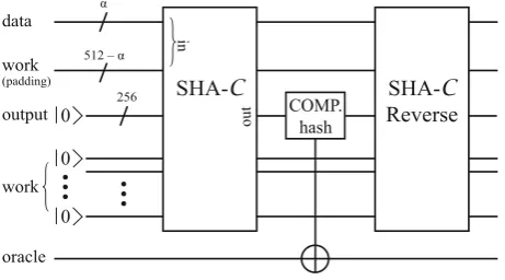
The idea of applying Grover’s algorithm to exhaustive attack on AES-128 is as follows. Linearly superposed 2128input keys encoded in 128 data qubits are fed as an input to AES-Cshown in Fig.7. AES-Ccontains a reversible circuit implementation of AES-128 encryption algorithm. The AES-Cencrypts the given plaintext, outputting superposed ciphertexts encoded in output qubits. Superposed ciphertexts are then compared with given ciphertext via C128NOT gate to mark the target. After marking is done, every qubit except the oracle qubit is passed on to AES-CReverse to disentangle the data qubits from other qubits.
oracle data
work
128
128
COMP. ciphertext
AES-C
in
out
0
AES-C
Reverse
output
0
0
5.1 Circuit implementation cost
AES-128 encryption internally performs SubBytes, MixColumns, ShiftRows, AddRoundKey, SubWord, RotWord, and Rcon. Quantum circuits for these operations are mostly adopted from [6] with improvements and fixes.
MixColumns, ShiftRows, and RotWord are linear operations acting on 32 bits that do not require any work qubit nor Toffoli gate. Among them, last two are simple bit permutations which require no quantum gates (by re-wiring) or at most SWAP gates. MixColumns needs to be treated more carefully as it is not a bit permutation. Treating each four-byte column of the internal state as a length-four vector, MixColumns is expressed as a matrix multiplication,
⎛ ⎜ ⎜ ⎝
s0,j s1,j s2,j s3,j
⎞ ⎟ ⎟ ⎠= ⎛ ⎜ ⎜ ⎝
02 03 01 01 01 02 03 01 01 01 02 03 03 01 01 02
⎞ ⎟ ⎟ ⎠ ⎛ ⎜ ⎜ ⎝
s0,j
s1,j
s2,j
s3,j
⎞ ⎟ ⎟
⎠, for 0≤ j ≤3, (18)
where 01, 02, 03 are submatrices when each bytesi,jis treated as a length-eight vector,
written as 01= ⎛ ⎜ ⎜ ⎜ ⎜ ⎜ ⎜ ⎜ ⎜ ⎜ ⎜ ⎝
1 0 0 0 0 0 0 0 0 1 0 0 0 0 0 0 0 0 1 0 0 0 0 0 0 0 0 1 0 0 0 0 0 0 0 0 1 0 0 0 0 0 0 0 0 1 0 0 0 0 0 0 0 0 1 0 0 0 0 0 0 0 0 1
⎞ ⎟ ⎟ ⎟ ⎟ ⎟ ⎟ ⎟ ⎟ ⎟ ⎟ ⎠
, 02=
⎛ ⎜ ⎜ ⎜ ⎜ ⎜ ⎜ ⎜ ⎜ ⎜ ⎜ ⎝
0 1 0 0 0 0 0 0 0 0 1 0 0 0 0 0 0 0 0 1 0 0 0 0 1 0 0 0 1 0 0 0 1 0 0 0 0 1 0 0 0 0 0 0 0 0 1 0 1 0 0 0 0 0 0 1 1 0 0 0 0 0 0 0
⎞ ⎟ ⎟ ⎟ ⎟ ⎟ ⎟ ⎟ ⎟ ⎟ ⎟ ⎠
, 03=
⎛ ⎜ ⎜ ⎜ ⎜ ⎜ ⎜ ⎜ ⎜ ⎜ ⎜ ⎝
1 1 0 0 0 0 0 0 0 1 1 0 0 0 0 0 0 0 1 1 0 0 0 0 1 0 0 1 1 0 0 0 1 0 0 0 1 1 0 0 0 0 0 0 0 1 1 0 1 0 0 0 0 0 1 1 1 0 0 0 0 0 0 1
⎞ ⎟ ⎟ ⎟ ⎟ ⎟ ⎟ ⎟ ⎟ ⎟ ⎟ ⎠ .
Since an explicit form of transformation matrix is given in Eq.18, the quantum circuit implementation of the matrix can be found by methods given in [49,50].
AddRoundKey and Rcon are XOR-ings of fixed-size strings which can also be efficiently realized by CNOT or X gates only.
SubBytes and SubWord are the only operations which require quantum resources. Since SubBytes and SubWord consist of 16 and 4 S-boxes, the S-box is the only operation to be carefully discussed.
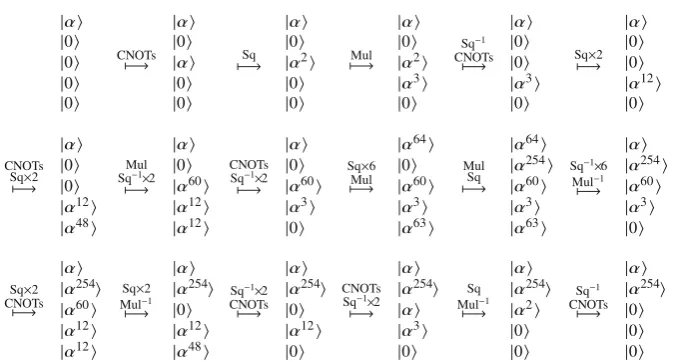
Classically, S-box can be implemented as a look-up table. However, a quantum counterpart of such table should involve the notion of the quantum memory aforemen-tioned in Sect.2.3. Therefore in this work, S-box is realized by explicitly calculating multiplicative inverse followed by affine transformations as described in Sect. 3.2.1 of [6].
S-box is realized by calculating multiplicative inverse followed by GF-linear map-ping and addition of S-box constant. By treating a byte as an element in GF(28)=
GF(2)[x]/(x8+x4+x3+x+1), GF-linear mapping and addition of S-box constant
Fig. 8 Finding multiplicative inverse ofαwith seven multipliers involved ⎛ ⎜ ⎜ ⎜ ⎜ ⎜ ⎜ ⎜ ⎜ ⎜ ⎜ ⎝ x0 x1 x2 x3 x4 x5 x6 x7 ⎞ ⎟ ⎟ ⎟ ⎟ ⎟ ⎟ ⎟ ⎟ ⎟ ⎟ ⎠ = ⎛ ⎜ ⎜ ⎜ ⎜ ⎜ ⎜ ⎜ ⎜ ⎜ ⎜ ⎝
1 0 0 0 1 1 1 1 1 1 0 0 0 1 1 1 1 1 1 0 0 0 1 1 1 1 1 1 0 0 0 1 1 1 1 1 1 0 0 0 0 1 1 1 1 1 0 0 0 0 1 1 1 1 1 0 0 0 0 1 1 1 1 1
⎞ ⎟ ⎟ ⎟ ⎟ ⎟ ⎟ ⎟ ⎟ ⎟ ⎟ ⎠ ⎛ ⎜ ⎜ ⎜ ⎜ ⎜ ⎜ ⎜ ⎜ ⎜ ⎜ ⎝ x0 x1 x2 x3 x4 x5 x6 x7 ⎞ ⎟ ⎟ ⎟ ⎟ ⎟ ⎟ ⎟ ⎟ ⎟ ⎟ ⎠ + ⎛ ⎜ ⎜ ⎜ ⎜ ⎜ ⎜ ⎜ ⎜ ⎜ ⎜ ⎝ 1 1 0 0 0 1 1 0 ⎞ ⎟ ⎟ ⎟ ⎟ ⎟ ⎟ ⎟ ⎟ ⎟ ⎟ ⎠ , (19)
where addition is XOR operation andxi are coefficients of polynomial of orderx7.
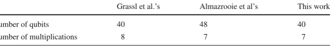
No work qubit nor Toffoli gate is required in this step. While XOR operation is simply done by applying X gates to relevant qubits, implementing a transformation matrix in Eq.19is not trivial. See [49,50] for general methods of realizing linear transformations. Resource estimate of quantum AES-128 encryption has been narrowed down to estimate the cost of finding multiplicative inverse of the elementαin GF(28). In [6], multiplicative inverse ofαis calculated by using two arithmetic circuits, Maslov et al.’s modular multiplier [51] and in-place squaring [6]. Slight modification of previ-ous method is found in this work with seven multipliers being used, verified by the quantum circuit simulation by matrix product state [52]. We visualize the sequence in a simplified way such that for example,|α|0|0|0|0−−−−→ |CNOTs α|0|α|0|0means CNOT gates are used to copy the string in the first eight-bit register to the third register. The entire sequence is given in Fig.8, where each state ket represents eight-bit register, and Sq and Mul denote modular squaring and multiplication operations. One can see that in Fig.8, only seven multipliers have been used. Almazrooie et al. also came up with a design for multiplicative inverse [4]. We briefly compare the existing circuit designs in Table1.
As squaring in GF(28) is linear, it does not involve the use of Toffoli nor work qubits.

![Fig. 6 Addition of two bitsab a and b in terms of a Toffoli and b T gates (Fig. 7(d) in [46])](https://thumb-us.123doks.com/thumbv2/123dok_us/7981659.1323937/23.439.54.386.54.138/fig-addition-bitsab-terms-toffoli-t-gates-fig.webp)