Grading Fruits and Vegetables Using RGB-D
Images and Convolutional Neural Network
著者
Nishi Toshiki, Kurogi Shuichi, Matsuo
Kazuya
journal or
publication title
2017 IEEE Symposium Series on Computational
Intelligence (SSCI)
year
2017-12-01
URL
http://hdl.handle.net/10228/00006888
Grading Fruits and Vegetables Using RGB-D
Images and Convolutional Neural Network
Toshiki Nishi
Department of Control Engineering Kyushu Institute of Technology
Kitakyushu, Japan [email protected]
Shuichi Kurogi
Department of Control Engineering Kyushu Institute of Technology
Kitakyushu, Japan [email protected]
Kazuya Matsuo
Department of Control Engineering Kyushu Institute of Technology
Kitakyushu, Japan [email protected]
Abstract—This paper presents a method for grading fruits and vegetables by means of using RGB-D (RGB and depth) images and convolutional neural network (CNN). Here, we focus on grading according to the size of objects. First, the method transforms positions of pixels in RGB image so that the center of the object in 3D space is placed at the position equidistant from the focal point by means of using the corresponding depth image. Then, with the transformed RGB images involving equidistant objects, the method uses CNN for learning to classify the objects or fruits and vegetables in the images for grading according to the size, where the CNN is structured for achieving both size sensitivity for grading and shift invariance for reducing position error involved in images. By means of numerical experiments, we show the effectiveness and the analysis of the present method.
Index Terms—grading fruits and vegetables according to size, RGB-D images, convolutional neural network, size sensitivity, shift invariance
I. INTRODUCTION
This paper presents a method for grading fruits and vegeta-bles by means of using RGB-D (RGB and depth) images and convolutional neural network (CNN). Here, grading of fruits and vegetables, in general, is sorting them into different grades according to the size, shape, color, volume, and so on, and we focus on grading according to the size in this paper. There are various methods using artificial neural networks and image processing for classification and grading of fruits and agricul-tural products as reviewed in [1]–[3], where features such as size, shape, color, texture, etc. are used for grading. However, no research study on grading using RGB-D images and CNN is reviewed, while, recently, a number of object classification and/or recognition methods using RGB-D images and CNNs are studied [4]–[6]. Although they have shown state-of-the-art performance in classification and/or recognition tasks, one of the problems to use CNNs for grading objects according to size is that the ability of CNNs for size invariant classification may be ineffective. Furthermore, CNNs require a fixed size input and widely used image warping approach [5] will cause loss of size information.
By means of considering these aspects, we have constructed a method as follows; first, the method transforms positions of pixels in RGB image so that the center of the object in 3D space is placed at the position equidistant from the focal point
by means of using the corresponding depth image. Then, with the transformed RGB images involving equidistant objects, the method uses CNN for learning to classify the objects for grading, where the CNN is structured for achieving both size sensitivity for grading and shift invariance for reducing position error involved in the images. We show the details of the method in II, experimental results and analysis inIII and conclusion inIV.
II. METHOD FORGRADINGOBJECTS USINGRGB-D IMAGES ANDCNN
A. Transformation for RGB Images Involving Equidistant Ob-jects
We make RGB images for training and learning as follows; suppose that we have RGB image G[RGB]ext and depth image
G[Depth]ext involving an object extracted with the size Wext×
Hext from original RGB-D images, G[RGB]orig and G [Depth]
orig .
Then, we first obtain the 3D point(x, y, z) corresponding to the pixel at(Xext, Yext)with depth valueDextinG[Depth]ext by
x=
Xext−0.5Wext
Wext
(2Dexttan(0.5θWext)), (1)
y=
Y
ext−0.5Hext
Hext
(2Dexttan(0.5θHext)), (2)
z=Dext, (3)
where θWext and θHext represent viewing angle of G
[Depth] ext
(see Fig. 1). In order to recognize an object invariantly with the distance to the object, we replace the 3D points of the object so that the mean position(xc, yc, zc)of the objects for all images is placed at the same position(0,0, zr), and then inversely transform to a depth image with the sizeW×H by
X =⌊ x−x c 2(z−zc+zr) tan(0.5θW) + 0.5 W⌋ (4) Y =⌊ y−yc 2(z−zc+zr) tan(0.5θH) + 0.5 H⌋ (5) D=⌊z−zc+zr⌋ (6) where θW andθH are viewing angles of new image, and ⌊·⌋ indicates the floor function. We useW =H = 100andθW =
x W X D z θW 0.5θW 3D-position (xz-plane) 2D tan(0.5θW) W X D depth image (X-axis) focal point target point
Fig. 1. Relationship between depthDat position(X, Y)in a depth image and 3D position(x, y, z)forY =y= 0. InterpretDext=D,Xext=X, Yext=Y,Wext=W for text.
θH = 100·57/320for the data of Kinect v1 in the experiment shown below.
The values (R, G, B) at the position (Xext, Yext) in the
original extracted RGB image G[RGB]ext is used for the
trans-formed image G[RGB] at(X, Y)as follows;
R(X, Y) =R(Xext, Yext) (7)
G(X, Y) =G(Xext, Yext) (8)
B(X, Y) =B(Xext, Yext) (9)
Here, since the resolution of G[RGB]andG[RGB]
ext is different,
there is a possibility that a position (X, Y)∈[0, W)×[0, H)
without the correspondence to (Xext, Yext) ∈ [0, Wext)×
[0, Hext)exists. Therefore, we have executed linear, quadratic
and no interpolation of RGB values for the position without correspondence, respectively, when it is surrounded by two, more than two and less than two positions with correspon-dence.
B. CNNs for Grading Objects According to Size
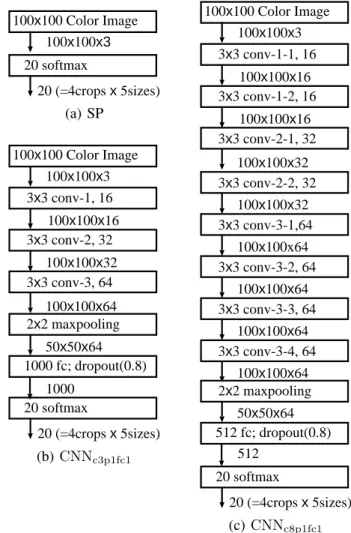
Now, we consider the grading of objects in RGB images according to the size. In research studies on neural network image processing [10], the convolutional neural network con-sisting of a convolutional layer and a max pooling layer, the cells in the convolutional layer work as learnable filters for extracting local features as simple cells in the visual cortex and the cells in the max pooling layer achieve small shift invariance as complex cells in the visual cortex. Furthermore, size (or scale) invariance is achieved by multiple convolutional and max pooling layers. However, in the grading task, size invariance should not be so large in order for grading the size while allowing small error of transformation arose in the process to obtain RGB images involving equidistant objects shown in the previous section. From this point of view, we have examined three neural networks shown in Fig. 2, where (a) is a simple neural network, which we call SP, and (b)
100x100 Color Image 100x100x3 20 (=4crops x 5sizes) 20 softmax (a) SP 100x100 Color Image 100x100x3 3x3 conv-1, 16 100x100x16 3x3 conv-2, 32 2x2 maxpooling 100x100x64 100x100x32 3x3 conv-3, 64 50x50x64 1000 fc; dropout(0.8) 1000 20 softmax 20 (=4crops x 5sizes) (b)CNNc3p1fc1 100x100 Color Image 100x100x3 3x3 conv-1-1, 16 100x100x16 3x3 conv-1-2, 16 2x2 maxpooling 100x100x32 3x3 conv-2-1, 32 512 fc; dropout(0.8) 512 20 softmax 20 (=4crops x 5sizes) 100x100x32 3x3 conv-2-2, 32 100x100x64 3x3 conv-3-1,64 3x3 conv-3-2, 64 3x3 conv-3-4, 64 3x3 conv-3-3, 64 100x100x64 100x100x64 100x100x64 50x50x64 100x100x16 (c)CNNc8p1fc1 Fig. 2. Example of neural networks for comparing the performance in grading objects according to the size. The activation function of the units in all convolutional layers and fully connected layer (fc) are ReLU (rectified linear unit). The dropout ratio for fc layer is 0.8. Output size of each layer is written at the right hand side of the output arc, e.g. “100x100x3” indicates the output size is given by the image consisting of 100×100 pixcels of 3 channels (RGB).
and (c) are CNNs, which we call CNNc3p1fc1 (involving 3
convolutional layers, a max pooling layer and a fully connected layer) and CNNc8p1fc1 (involving 8 convolutional layers, a
max pooling layer and a fully connected layer), respectively. As learning algorithm, we have used Adam optimizer. Here, note that the structure and the function of the constituent layers, such as convolutional, max pooling, fully connected and softmax layres, and Adam learning optimizer are standard in deep learning architectures [9], [10]. Moreover, we have implemented these neural networks in the Chainer framework [8] as one of the standard frameworks.
One of the most important structure is that we have placed only one max pooling layer for the last convolutional layer, or conv-3 forCNNc3p1fc1 and conv-3-4 forCNNc8p1fc1. We
have obtained this structure as the best one among 8 = 23
combinations of whether we use or not max-pooling layers for convolutional layers (conv-1, conv-2, conv-3 for CNNc3p1fc1
and conv-1-2, conv-2-2, conv-3-4 forCNNc8p1fc1). The reason
Fig. 3. Example of three images of apple (upper left), bell pepper (upper right), orange (lower left) and tomato (lower right), respectively, where the three images are original RGB image (left), depth image (middle), and training RGB image (right) consisting of transformed object and training background image.
image size from100×100into a half50×50and further size reduction may not be useful for grading objects according to the size.
C. Learning for Rotation Invariance
In order for rotation invariance, we have trained the net-works shown in Fig. 2 with rotated images of the objects. As shown in the experiments described below, we have used the images of objects on a turntable rotated around y-axis (or vertical direction), and we rotate the objects in the image aroundz-axis (or depth direction) by transforming the images, while we do not have used the rotation around x-axis which is for our future research studies.
D. Color spaces
For color dependent grading, we have evaluated the perfor-mance for three color spaces, RGB, HSV (hue, saturation, and value), and HSL (hue, saturation, and lightness), where HSV and HSL are occasionally used in color detection in robot vision [11], [12].
III. NUMERICALEXPERIMENTS ANDANALYSIS
A. Training and Test Datasets
We have examined the present methods for grading objects with the Washington RGB-D object dataset [13]. This dataset was recorded using a Kinect style 3D camera that records synchronized and aligned 640×480 RGB and depth images at 30 Hz. Each object was placed on a turntable and video sequences were captured for one whole rotation, and has different number of images. Namely, we have used four objects of fruits and vegetables named apple 1 1, bell pepper 1 1, orange 1 1, and tomato 1 1, each of which has 208, 193, 195, and 249 images, respectively. From the first 180 images for each object, odd-number images are used for training, and even-number images are used for test. From each image, we make five different sizes of objects magnified by the ratio 0.8, 0.9, 1.0, 1.1 and 1.2. Furthermore, each magnified object is rotated randomly in the range −10 to 10 degrees around z -axis. Thus, we have5400 = 4×5×3×90images in each of
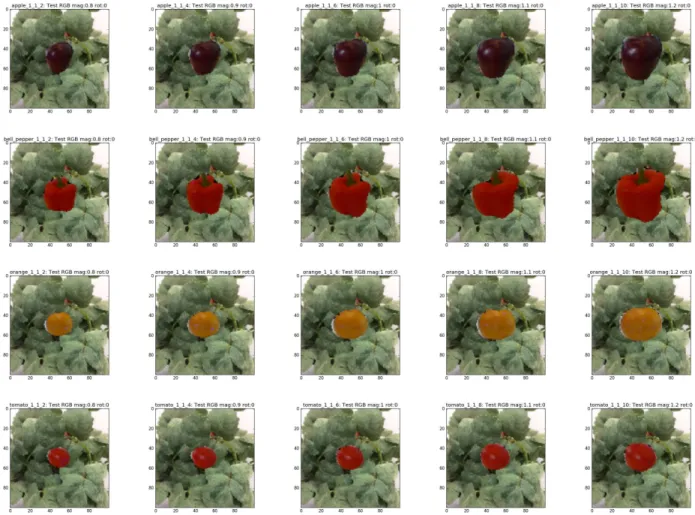
training and test datasets. We classify 20 classes consisting of five sizes of four fruits and vegetables (apple, bell pepper, orange and tomato). Thus, each class has 270 images for RGB and depth. For training and test RGB images, different backgrounds of the objects as shown in Fig. 3 and Fig. 4. B. Experimental Results and Analysis
We show experimental result of the loss (cross-entropy) and
NLACC(negative log accuracy) for training and test dataset vs. the number of learning epochs in Fig. 5. Here, the cross-entropy is defined by E,− N X n=1 K X k=1 dnklogynk (10) for the output vectoryn= (yn1, yn2,· · ·, ynK)of the network and the target vectordn= (dn1, dn2,· · ·, dnK)w.r.t. the input vector xn (n = 1,2,· · ·, N). Here, dnk = 1 if xn is in the
kth class, and 0 otherwise. On the other hand, the accuracy is defined by ACC, 1 N N X n=1 1 ( argmax k=1,···,K dnk= argmax k=1,···,K ynk ) . (11)
where 1{z} denotes an indicator function equals to 1 if z
is true, and 0 otherwise. Furthermore, we define NLACC,
−log(ACC)for explaining the result from a different point of view of the loss as shown below. When1−ACC≪1, we have
NLACC =−log(ACC)≃1/ACC, e.g.NLACC≃0.1, 0.01 and0.001 for ACC = 0.9, 0.99 and 0.999, respectively.
From the training and test loss in Fig. 5, we can see that CNNs (CNNc3p1fc1 and CNNc8p1fc1) have achieved better
performance than SP from the point of view of the magnitude of fluctuation and ACC achieved at 200 learning epochs. Here, we have reduced the magnitude of fluctuation by a large dropout ratio 0.8 for the CNNs, but we do not have optimized other parameters such as number of units, number of filters, and so on to obtain better performance. Furthermore, we could not have obtained reasonable learning result for RGB and
Fig. 4. Example of test images consisting of transformed objects magnified by the ratio 0.8, 0.9, 1.1 and 1.2 and test background image.
HSV with CNNc8p1fc1, which is considered to be owing to
the vanishing gradient problem and we have applied the batch normalization method but we could not have reasonable result. We would like to solve this problem in our future research studies.
We can observe the overfitting for all cases from the point of view that test loss is larger than training loss. Furthermore, the curve of test loss for CNNc3p1fc1 and SP increases with the
increase of the number of learning epochs, which indicates a phenomenon of increasing overlearning. However, we can see that NLACC decreases with the increase of the number of epochs. Since the learning algorithm is for reducing training loss, this phenomenon is not easy to understand. Since the ultimate objective of learning for this task is to increase
ACC or decreaseNLACCfor test dataset, this phenomenum may indicate a mismatch between learning objective and the learning algorithm for reducing the loss defined by the cross entropy of the output of CNN. From another point of view, we suspect that training and test images are very similar, and the generalization ability of learning algorithm (decreasing test loss) is not so necessary, which indicates inadequate test images. However, the test loss forCNNc8p1fc1 decreases with
the increase of the number of epochs, which indicates that the
generalization ability is obtained by modifying the structure of CNN. We would like to clarify this phenomenum in our future research studies.
By means of comparing the performance obtained for RGB, HSV and HSL color spaces shown in Fig. 5, we may say that HSL is superior to HSV and HSV is superior to RGB, while the difference does not seem so large.
In Table I, we show the confusion matrix achieved by
CNNc3p1fc1 at 200 learning epochs. We can see that the
performance is good, and the most characteristic grading error occurs for the adjacent sizes for each fruit. Since the CNNs using max pooling layers for conv-1 and conv-2 has provided worse result not in the classification of the name of fruits and vegetables but in the classification of the sizes (not shown in this paper), we can say that max pooling layer with the last convolutional layer plays an important role in grading the objects according to the size.
IV. CONCLUSION
We have presented a method of grading fruits and vegetables by means of using RGB-D images and CNN. The method remakes RGB images involving equidistant objects by means of using depth image, and then utilizes CNN for learning to
trai n in g lo ss 0.001 0.01 0.1 1 10 100 1000 10000 0 200 RGB HSV HSL number of epochs 50 100 150 0.001 0.01 0.1 1 10 100 1000 10000 0 200 RGB HSV HSL number of epochs 50 100 150 0.001 0.01 0.1 1 10 100 1000 10000 0 50 100 150 200 number of epochs RGB HSV HSL tes t lo ss 0.001 0.01 0.1 1 10 100 1000 10000 0 200 number of epochs RGB HSV HSL 50 100 150 0.001 0.01 0.1 1 10 100 1000 10000 number of epochs RGB HSV HSL 0 50 100 150 200 0.001 0.01 0.1 1 10 100 1000 10000 0 50 100 150 200 number of epochs RGB HSV HSL trai n in g N L A C C 0.001 0.01 0.1 1 10 0 50 100 150 200 number of epochs RGB HSV HSL 0.001 0.01 0.1 1 10 0 50 100 150 200 number of epochs RGB HSV HSL 0.001 0.01 0.1 1 10 0 50 100 150 200 number of epochs RGB HSV HSL tes t N L A C C 0.001 0.01 0.1 1 10 0 50 100 150 200 number of epochs RGB HSV HSL 0.001 0.01 0.1 1 10 0 50 100 150 200 number of epochs RGB HSV HSL 0.001 0.01 0.1 1 10 0 50 100 150 200 number of epochs RGB HSV HSL (a) SP (b) CNNc3p1fc1 (c)CNNc8p1fc1
Fig. 5. Experimental result of loss and NLACC for training and test dataset vs. the number of learning epochs. The accuracy,ACC, for test dataset achieved at 200 epochs with HSL, HSV, RGB images is 0.955, 0.909, 0.732 by SP, 0.979, 0.967, 0.929 byCNNc3p1fc1, and 0.981 byCNNc8p1fc1with HSL.
classify RGB images for the grading of objects according to the size, where the CNN is structured for achieving both size sensitivity for grading and shift invariance for reducing error involved in RGB images. By means of numerical experiment, we have shown the effectiveness and the analysis of the method. For easy experiments in this paper, we have generated the images of different size objects by transforming original images, while we are now conducting to use RGB-D images involving actual different sizes of objects as well as actual rotated objects and actual background of objects. Furthermore, we would like to examine the parameters of CNN much more and optimize them for the grading of objects according to not only the size but also other features.
REFERENCES
[1] J. Gill, P.S. Sandhu, T. Singh, “A Review of Automatic Fruit Classifi-cation using Soft Computing Techniques,” International Conference on Computer, Systems and Electronics Engineering (ICSCEE’2014), pp.91– 98, 2014
[2] M. Raj, D. Swaminarayan, “Applications of Image Processing for Grading Agriculture products,” International Journal on Recent and Innovation Trends in Computing and Communication, 3(3), pp.1194– 1201, 2015
[3] S. Banot, P.M. Mahajan, “A Fruit Detecting and Grading System Based on Image Processing-Review,” International Journal of Innova-tive Research in Electrical, Electoronics, Instrumentation and Control Engineering, 4(1), 2016
[4] R. Socher, B. Huval, B. Bhat, C.D. Manning, A.Y. Ng, “Convolutional-Recursive Deep Learning for 3D Object Classification,” Advances in Neural Information Processing Systems 25 (NIPS 2012), 2012 [5] A. Eitel,J.T. Springenberg, L. Spinello, M. Riedmiller,W. Burgard,
TABLE I
CONFUSION MATRIX OF GRADING RESULT BYCNNc3p1fc1WITHACC=0.979OBTAINED AT200EPOCHS. THE NAME OF FRUIT AND VEGETABLE IN THE FIRST COLUMN AND THE FIST ROW INDICATE ACTUAL AND CLASSIFIED NAME OF THE OBJECT,RESPECTIVELY. THE SECOND COLUMN AND THE SECOND
ROW INDICATE THE ACTUAL AND GRADED SIZE,RESPECTIVELY.
apple bell pepper orange tomato
0.8 0.9 1.0 1.1 1.2 0.8 0.9 1.0 1.1 1.2 0.8 0.9 1.0 1.1 1.2 0.8 0.9 1.0 1.1 1.2 ap p le 0.8 270 0 0 0 0 0 0 0 0 0 0 0 0 0 0 0 0 0 0 0 0.9 1 268 0 1 0 0 0 0 0 0 0 0 0 0 0 0 0 0 0 0 1.0 0 4 263 3 0 0 0 0 0 0 0 0 0 0 0 0 0 0 0 0 1.1 0 0 2 266 2 0 0 0 0 0 0 0 0 0 0 0 0 0 0 0 1.2 0 0 0 3 265 0 0 0 1 1 0 0 0 0 0 0 0 0 0 0 b el l p ep p er 0.8 0 0 0 0 0 266 2 1 0 0 0 0 0 0 1 0 0 0 0 0 0.9 0 0 0 0 0 5 256 9 0 0 0 0 0 0 0 0 0 0 0 0 1.0 0 0 0 0 0 0 3 264 3 0 0 0 0 0 0 0 0 0 0 0 1.1 0 0 0 0 0 0 0 9 256 5 0 0 0 0 0 0 0 0 0 0 1.2 0 0 0 0 0 0 0 1 1 268 0 0 0 0 0 0 0 0 0 0 o ran g e 0.8 0 0 0 0 0 0 0 0 0 0 269 0 0 0 0 0 0 1 0 0 0.9 0 0 0 0 0 0 0 0 0 0 0 270 0 0 0 0 0 0 0 0 1.0 0 0 0 0 0 0 0 0 0 0 0 0 269 1 0 0 0 0 0 0 1.1 0 0 0 0 0 1 0 0 0 0 0 0 0 269 0 0 0 0 0 0 1.2 0 0 0 0 0 1 0 0 0 0 0 0 0 0 269 0 0 0 0 0 to m at o 0.8 0 0 0 0 0 0 0 0 0 0 0 0 0 0 0 263 7 0 0 0 0.9 0 0 0 0 0 0 0 0 1 0 0 0 0 0 0 2 259 8 0 0 1.0 0 0 0 0 0 0 0 0 0 0 1 0 0 0 0 0 4 259 6 0 1.1 0 0 0 0 0 0 0 0 0 0 0 1 0 0 0 0 0 9 249 11 1.2 0 0 0 0 0 1 0 0 0 0 0 0 0 0 0 0 0 0 2 267
“Multimodal Deep Learning for Robust RGB-D Object Recognition,” IEEE/RSJ International Conference on Intelligent Robots and Systems (IROS), 2015
[6] C.R. Qi, H. Su,M. Niessner,A. Dai,M. Yan,L.J. Guibas, “Volumetric and Multi-View CNNs for Object Classification on 3D Data,” 2016 IEEE Conference on Computer Vision and Pattern Recognition (CVPR), 2016 [7] T.Kamishima , H. Asho, M. Yasuda, S. Maeda, D. Okanohara, T. Okaya, Y. Kubo, D. Bollegala, “Deep Learning (in Japanese),” Kindai Ka-gakusha, 2015
[8] S. Tokui, K. Oono, S. Hido, J. Clayton, “Chainer: A next-generation open source framework for deep learning,” in Workshop on Machine Learning Systems at Neural Information Processing Systems, 2015 [9] T. Okaya, “Machine Learning Professional Series: Deep Learning,”
Kodansha, Tokyo, 2015 (in Japanese)
[10] T. Kamishima (Ed.), “Deep Learning,” Kindaikagakusha, 2015 (in Japanese)
[11] S. Peng, Y. Wen, “Research based on the HSV humanoid robot soccer image processing,” Proc. of the International Conference on Communi-cation Systems, pp.52–55, 2010
[12] S.H. Tsai, Y.H. Tseng, “A novel color detection method based on HSL color space for robotic soccer competition,” Computers and Mathematics with Applications, 64(5), pp.1291–1300, 2012
[13] K. Lai, L. Bo, X. Ren, D. Fox, “A large-scale hierarchical multiview rgb-d object rgb-dataset,” Proc. of the IEEE Int. Conf. on Robotics & Automation (ICRA), 2011