Evolutionary algorithms for robust methods

econ

stor

www.econstor.eu

Der Open-Access-Publikationsserver der ZBW – Leibniz-Informationszentrum Wirtschaft

The Open Access Publication Server of the ZBW – Leibniz Information Centre for Economics

Nutzungsbedingungen:

Die ZBW räumt Ihnen als Nutzerin/Nutzer das unentgeltliche, räumlich unbeschränkte und zeitlich auf die Dauer des Schutzrechts beschränkte einfache Recht ein, das ausgewählte Werk im Rahmen der unter

→ http://www.econstor.eu/dspace/Nutzungsbedingungen nachzulesenden vollständigen Nutzungsbedingungen zu vervielfältigen, mit denen die Nutzerin/der Nutzer sich durch die erste Nutzung einverstanden erklärt.

Terms of use:

The ZBW grants you, the user, the non-exclusive right to use the selected work free of charge, territorially unrestricted and within the time limit of the term of the property rights according to the terms specified at

→ http://www.econstor.eu/dspace/Nutzungsbedingungen By the first use of the selected work the user agrees and declares to comply with these terms of use.

zbw

Nunkesser, Robin; Morell, Oliver

Working Paper

Evolutionary algorithms for robust

methods

Technical Report // Sonderforschungsbereich 475, Komplexitätsreduktion in Multivariaten Datenstrukturen, Universität Dortmund, No. 2008,29

Provided in cooperation with: Technische Universität Dortmund

Suggested citation: Nunkesser, Robin; Morell, Oliver (2008) : Evolutionary algorithms for robust methods, Technical Report // Sonderforschungsbereich 475, Komplexitätsreduktion in Multivariaten Datenstrukturen, Universität Dortmund, No. 2008,29, http://

Evolutionary Algorithms for Robust Methods

a_{Faculty of Computer Science, TU Dortmund University, Germany} b_{Faculty of Statistics, TU Dortmund University, Germany}

Abstract

A drawback of robust statistical techniques is the increased computational effort often needed compared to non robust methods. Robust estimators possessing the exact fit prop-erty, for example, are NP-hard to compute. This means that—under the widely believed assumption that the computational complexity classes NP and P are not equal—there is no hope to compute exact solutions for large high dimensional data sets. To tackle this problem, search heuristics are used to compute NP-hard estimators in high dimen-sions. Here, an evolutionary algorithm that is applicable to different robust estimators is presented. Further, variants of this evolutionary algorithm for selected estimators— most prominently least trimmed squares and least median of squares—are introduced and shown to outperform existing popular search heuristics in difficult data situations.

The results increase the applicability of robust methods and underline the usefulness of evolutionary computation for computational statistics.

Key words: Evolutionary algorithms, robust regression, least trimmed squares (LTS),

least median of squares (LMS), least quantile of squares (LQS), least quartile difference (LQD)

1. Introduction

Since the works of Box (1953) and Tukey (1960) the need for robust methods is apparent. The strong sensitivity of classical procedures to seemingly negligible deviations from the distributional assumptions calls for robust alternatives. In linear regression, positive-breakdown methods (Rousseeuw, 1997) are among the most important robust techniques. Unfortunately, the computation of these estimators is quite hard. More precisely, Bernholt (2005) shows that estimators with theexact fit property (whenever a majority of the observations lies on a hyperplane, an estimator with the exact fit property yields that hyperplane as the solution, see e.g. Rousseeuw, 1984) are NP-hard to compute. When accepting the widely believed assumption that the complexity classes NP and P are not equal (see e.g. Wegener, 2005 for an introduction to complexity theory),

I_{The financial support of the Deutsche Forschungsgemeinschaft (SFB 475, Reduction of complexity} in multivariate data structures) is gratefully acknowledged.

Email addresses: [email protected](Robin Nunkesser),

we therefore have no hope to compute exact solutions for large high dimensional data sets.

A typical approach to tackle problems we cannot compute exactly is to use heuristics. Evolutionary computation (see e.g. De Jong, 2006) is a well established search heuristic in computer science and steadily gaining importance in computational statistics. Exam-ples for the application of evolutionary computation in computational statistics include evolutionary clustering (Hruschka et al., 2006), association studies (Nunkesser et al., 2007), computation of robust estimators (Meyer, 2003; Morell et al., 2008), time series modeling (Baragona et al., 2004), and many more. Actually, the evolutionary algorithm presented by Morell et al. (2008) is the basis of the algorithm, we present here. We extend this algorithm to a framework that is applicable to different estimators, like the algorithm PROGRESS (Program for Robust Regression) (Rousseeuw and Leroy, 1987; Rousseeuw and Hubert, 1997) which is based on using subsamples of the data. Here, we concentrate on three robust estimators: least median of squares (LMS) (more precisely its generalization least quantile of squares (LQS)) and least trimmed squares (LTS), both proposed by Rousseeuw (1984) and as the third estimator least quartile difference (LQD) by Croux et al. (1994). Section 2 describes these estimators.

Section 3 provides a basic introduction to evolutionary computation, which is the basis of the algorithm presented in Section 4. In the final sections 5 and 6, we compare our algorithm to existing popular search heuristic and draw conclusions.

2. The Estimators LQS, LTS, and LQD

We consider the linear multiple regression model

yi=β0+β1xi1+. . .+βpxip+εi i= 1, . . . , n

whereβ0is an intercept term andεimodels statistical errors. Thep-dimensional vectors

xi= (xi1, . . . , xip)contain the explanatory variables andyi the response. For estimated

regression coefficientsβˆ1, . . . ,βˆp and an estimated interceptβˆ0, we denote the residuals

as ri ˆ β0, . . . ,βˆp =yi− ˆ β0+ ˆβ1xi1+. . .+ ˆβpxip .

Further, letui:n denote thei-th order statistic ofnnumbersu1, . . . , un. The estimators

we consider are defined as follows:

Definition 1 (Rousseeuw, 1984; Croux et al., 1994). Letribe theith residual

de-termined by a linear regression with parametersβˆ0, . . . ,βˆp and a given data setZ.

Theleast quantile of squares (LQS),least trimmed squares (LTS), andleast quartile

difference (LQD) estimates are given by

LQS (Z) = argmin ˆ β0,...,βˆp {r2₁, . . . , r2_n}hp:n LTS (Z) = argmin ˆ β0,...,βˆp hp X i=1 {r2₁, . . . , r_n2}i:n LQD (Z) = argmin ˆ β0,...,βˆp {|ri−rj|;i < j}₍hp 2):( n 2)

wherehp with1≤hp≤nis a parameter influencing the estimation.

LQS generalizes the least median of squares (LMS), defined as LMS (Z) = argmin

ˆ

β0,...,βˆp

med{r2₁, . . . , r2_n} .

Note also, that of course theleast trimmed sum of absolute values (LTA) proposed by Hössjer (1994) and defined as

LTA (Z) = argmin ˆ β0,...,βˆp hp X i=1 {|r1|, . . . ,|rn|}i:n

may also be computed by our algorithm. All these estimators are high-breakdown meth-ods, possessing the asymptotic breakdown point (Donoho and Huber, 1983) of50%for the appropriate choice ofhp. This means that almost 50% of the observations may be

contaminated without having unbounded effect on the estimate. LQS and LMS have the disadvantage of a low efficiency at Gaussian samples, which is asymptotically 0% (Croux et al., 1994). Arguments for LQS/LMS used to be the easier computation of the objective function compared to LTS and LQD—though the computation of the estima-tors is still NP-hard—and the intuitive definition. LTS and LQD are alternatives with higher asymptotic Gaussian efficiencies of7.1%and 67.1%, respectively. An additional advantage of LTS is its smooth objective function leading to a lower sensitivity to local effects (Rousseeuw and Van Driessen, 2006).

Because of the above mentioned advantages and disadvantages, the considered esti-mators are relevant for different data situations. Therefore, algorithms for them are of high interest. We consider situations where exact algorithms are not feasible and concen-trate on heuristics. The heuristics most commonly used are PROGRESS for LQS/LMS and LTS (Rousseeuw and Leroy, 1987; Rousseeuw and Hubert, 1997) and FAST-LTS for LTS (Rousseeuw and Van Driessen, 2006). LQD may be computed with LQS algorithms with a quadratic blow up of computation time (Croux et al., 1994). Aside from the best known heuristics, Hawkins and Olive (1999) propose a so called feasible solution algorithm (FSA) for LQS/LMS and LTS. The FSA is based on sampling data subsets of sizehp and iterative swapping of data points in the sample with data points outside the

sample.

3. Evolutionary Computation

The idea of evolutionary computation is to mimic the Darwin–Wallace principle of natural selection in order to obtain an efficient search heuristic. Evolution’s main prin-ciple is that populations of individuals evolve through variational inheritance where a concept of fitness reflects the ability to survive. Transfered to optimization, the popu-lation of individuals is a collection of candidate solutions, where the fitness reflects the goodness of the candidate solution, e.g. the objective value.

Individuals may be characterized bygenotypes (the genetic makeup) or phenotypes (observed qualities) or in algorithmic terms the computer representation of the candi-date solution and its (mathematical) interpretation if not apparent. Essential modules of evolutionary algorithms are therefore the fitness function that maps individuals to

fitness values, the genotype search space and an optional mapping between genotype and phenotype.

Further, selection schemes determining which individuals are selected for variation, and concepts to modify individuals are needed (typically calledmutation or

recombina-tion/crossover depending on whether one or more individuals are involved).

By nature, an evolutionary process is infinite. To obtain an algorithm that terminates, we additionally need astopping criterion.

The basic evolutionary process used by evolutionary algorithms is described in Algo-rithm 1.

Algorithm 1 (Basic Evolutionary Algorithm).

1. Create an initial random population.

2. Perform the following steps on the currentgeneration of individuals: (a) Select individuals in the population based on a selection scheme. (b) Adapt the selected individuals.

(c) Evaluate the fitness value of the adapted individuals.

(d) Select individuals for the next generation according to a selection scheme. 3. If the stopping criterion is fulfilled, then output the final population. Otherwise,

set the next generation as current and go to step 2.

Evolutionary computation is a very general and adaptive framework and ideas used in evolutionary algorithms can also be found in existing algorithms for robust regression. For example, the point interchange used by Hawkins (1993) in his feasible set algorithm to compute LMS can be seen as a mutation operator.

4. Outline of the Algorithm

As a first step, we have to appoint the genotype of the individuals, we work on. In order to have a limited number of candidate solutions, we restrict ourselves to candidate solutions uniquely determined by a data subsample of fixed size. In the most common algorithms PROGRESS and FAST-LTS the subsamples are for sound reasons of size

p. These reasons include the fact, that p linear independent points uniquely define a hyperplane. Additionally, smaller subsamples decrease the possibility of having outliers in the subsample. Although, strictly speaking, we are computing a different estimator when using subsamples of sizep, it remains being a high breakdown estimator (Rousseeuw and Basset Jr., 1991). We will adopt this in letting for explanatory dataZe={x1, . . . , xn} ⊂

Rp G= ( (g1, . . . , gn)∈ {0,1}n: n X i=1 gi=p )

be the genotype of our individuals that is mapped to its phenotype by the function

m:G→ {U ⊆_Rp_{:|U|=p} with}

m((g1, . . . , gn)) ={xi ∈Ze;gi= 1} .

Thus, we obtain n_p

different possible individuals. The determination of the fitness or goodness of these individuals comprises two steps:

1. Compute a unique candidate solution hyperplaneH from the given individual. 2. Compute—depending on the estimator chosen—one of the three objective functions

{r2 1, . . . , rn2}hp:n, Php i=1{r 2 1, . . . , r2n}i:n, or {|ri−rj|;i < j}₍hp 2):( n 2) (the residuals ri

are determined byH and the given data). The algorithm we propose is the following:

Algorithm 2 (Evolutionary Algorithm for Robust Regression).

1. Select(g1, . . . , gn)∈Guniformly at random, constituting the initial population.

(a) Compute a unique hyperplaneH from(g1, . . . , gn).

(b) Determine the objective valuef for the chosen estimator. 2. Perform the following steps on the current individual(g1, . . . , gn):

(a) Conduct one of the following adaptions chosen uniformly at random:

i. Randomly select gi, gj ∈ (g1, . . . , gn) with gi 6= gj and exchange their

values to obtain(g0₁, . . . , g0_n).

ii. Randomly selectk > pand compute the index setI defined by

i∈ {1, . . . , n};r_i2∈ {r2₁, . . . , r_n2}(k−p+1):n∪. . .∪ {r12, . . . , r 2

n}k:n

whereri are residuals defined byH. Setg0i∈(g01, . . . , g0n)to1 iffi∈I.

iii. Select(g0₁, . . . , g0_n)∈Guniformly at random. (b) Compute a unique hyperplaneH0 from(g10, . . . , gn0).

(c) Determine the objective valuef0 for the chosen estimator. (d) If f0< f set(g1, . . . , gn) = (g01, . . . , g0n),H =H0, andf =f0.

3. If either

(a) the elapsed time,

(b) the number of adaptions conducted, or

(c) the number of adaptions without improved objective value

exceeds its predetermined maximum, stop and output the final individual. Other-wise go to step 2.

The main difference to PROGRESS and FAST-LTS is that we have a continuous process changing subsamples instead of drawing a fixed number of subsamples. Thus, we are better able to use the information of good candidate solutions. Only using the mutation 2(a)i would lead to staying in local optima. The adaption described in 2(a)ii redeems this disadvantage in potentially moving far away from local optima, but still us-ing information contained in the solution. Note, that the effect is similar to the adaption “move” described by Morell et al. (2008), but the adaption proposed here is simpler to compute. The adaption 2(a)iii introduces resampling to the algorithm.

The question how to compute a unique hyperplane from a subset of sizepremains. As a first step, we compute the hyperplaneH through the subset of data points. If it does not define a unique hyperplane, we try to add observations in fixed order (e.g. starting with x1) until it does. The second step depends on the estimator and is described in

more detail in the following. A third optional step is to adjust the intercept of the unique hyperplane by doing an LTS/LQS/LQD univariate estimate on the residuals defining the objective value (Rousseeuw and Hubert, 1997). We include this step in our algorithm.

4.1. Computing a Unique Hyperplane for LTS

Rousseeuw and Van Driessen (2006) show that the following procedure guarantees an improvement in the objective value of the LTS estimateH:

1. Determine thehp points with the lowest squared residuals with regard toH.

2. Compute the least squares fit hyperplaneH0 on thesehppoints.

4.2. Computing a Unique Hyperplane for LQS

The situation for LQS is more complex. The following procedure also guarantees an improvement in objective value (Stromberg, 1993):

1. Determine thehp points with the lowest squared residuals with regard toH.

2. Compute a minimax fit hyperplaneH0 on thesehp points defined by

argmin

ˆ

β0,...,βˆp

max{r2₁, . . . , r2_hp}

wherer1, . . . , rhp are the residuals of the chosenhp points.

One possibility to compute such a fit is based on computing least squares fits on all

hp

p+1

possible subsamples of size p+ 1 (Stromberg, 1993). For large hp or p this is

clearly prohibitive. A second possibility is to do a least squares fit on a subset of the data uniquely defined byH. We propose to use least squares on thehp points with the

smallest squared residuals with regard toH. This often leads to an improved objective value, but different to LTS regression the improvement is not guaranteed. Thus we only chooseH0 instead ofH as the unique hyperplane, ifH0 leads to a better objective value. A third possibility to improve the objective value is to do weighted least squares on the data points with the lowest squared residuals with regard toH and give higher weight to the data points with higher residuals.

4.3. Computing a Unique Hyperplane for LQD

The similarity of LQD to LQS allows us to use the following procedure to obtain a guaranteed better objective value:

1. Determine the set of points Z ={(xi−xj, yi−yj)} such that the corresponding

absolute residual differences|ri−rj|with regard toH are among thehp smallest.

2. Compute a minimax fit hyperplaneH0 onZ.

It is easy to see, that this procedure guarantees a better objective value, because Croux and Rousseeuw (1992) showed that it is possible to compute the LQD by computing an LQS on the data set of differences {(xi−xj, yi−yj) ; 1 ≤i < j ≤}. This is however,

due to a typically largerhp than in LQS estimation, even more prohibitive than in case

of the LQS for largehp or p. Again, a good alternative is to use least squares fits on

subsets of the data (this time on the according data sets of differences).

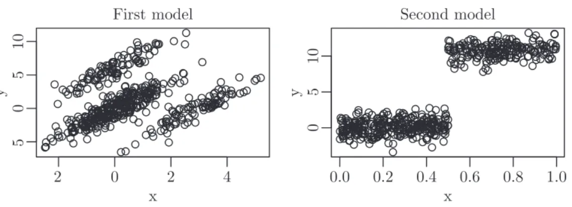
�2 0 2 4 �5 05 10 First model x y 0.0 0.2 0.4 0.6 0.8 1.0 05 10 Second model x y

Figure 1: Example of simulated data forp= 1.

5. Comparison

We compare our algorithm with results from PROGRESS for LQS and results from FAST-LTS for LTS. We omit the LQD, because—as we have seen—a transformation to LQS exists and to our knowledge, no implementation of LQD algorithms for high dimensional data exist. PROGRESS is implemented in the function lqs of the R (R Development Core Team, 2008) package MASS (Venables and Ripley, 2002) and FAST-LTS is implemented in the functionltsRegof the R package robustbase (Todorov et al., 2007). Our own algorithms are implemented in the funtionrobreg.evolof the R package RFreak (Nunkesser, 2008).

To compare the algorithms, we simulate data with n = 500 data points for p = 1, . . . ,30 from two different models. In the first model, the independent regressors are normally distributed. In the second model, they stem from a uniformly distributed random design on the interval(0,1). The first model is given by

yi=β0+β1xi1+. . .+βpxip+εi i= 1, . . . , n

whereβ0 is an intercept term andεi∼ N(0,1)are statistical errors. The parameterβ0

is set to 0, while β1, . . . βp equal 2. We add 40% outliers to the data in choosing two

disjunct samples of size20%. We add 3 to the explanatory data in the first sample and 6 to the response in the second sample, generating additive outliers in the explanatory and the response variables, respectively.

The second model contains a structural change. The parameterβ1is1, whileβ2, . . . βp

are0. Thus, the corresponding regressors add only noise to the problem. The structural change is in the intercept, which is

β0=

0, ifxi1≤ {xj1; 1≤j≤500}300:500

10, ifxi1>{xj1; 1≤j≤500}300:500

.

A good robust estimate ofβ should giveβ0 close to0and the slopes as above. Figure 1

shows an example of two simulated data sets based on these models withp= 1.

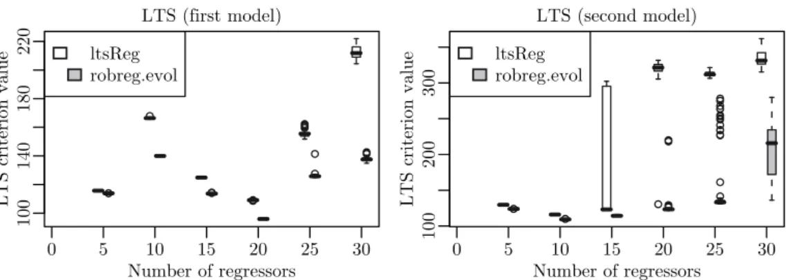
To compare the algorithms fairly, we measure the runtimelqs andltsReg, respec-tively, need for the computation and give our algorithm exactly the same amount of time. Figure 2 shows the results for LTS and Figure 3 shows the results for LMS.

100 140 180 220 LTS (first model) Number of regressors LTS criterion valu e 0 5 10 15 20 25 30 ltsReg robreg.evol 100 200 300 LTS (second model) Number of regressors LTS criterion valu e 0 5 10 15 20 25 30 ltsReg robreg.evol

Figure 2: Comparison of robreg.evolwithltsReg.

01 02 03 04 05 0 LMS (first model) Number of regressors LMS criterion valu e 0 5 10 15 20 25 30 lqs robreg.evol 234567 LMS (second model) Number of regressors LMS criterion valu e 0 5 10 15 20 25 30 lqs robreg.evol

Figure 3: Comparison ofrobreg.evolwithlqs.

In nearly all conducted runs, our algorithm achieves better results than the established algorithmslqs and ltsReg. Another observation is, that the structural change in the second data set affects the LTS estimation of ltsRegheavily forp≥15while the effect onrobreg.evol is far less. All in all, robreg.evol seems to be better suited for the considered data situations.

6. Conclusion

Many high breakdown estimators are in all likelihood not computable exactly in high dimensional regressor spaces. The common heuristics to compute solutions in these cases work with subsample versions of the estimators. In demanding data situations with a high percentage of contamination, the existing algorithms do not work well. The algorithm we propose is able to handle a high percentage of contamination in a high dimensional regressor space. In addition, it also provides superior results on data with less contamination and lower dimension considered in this paper. It therefore is a considerable alternative to the popular algorithms PROGRESS and FAST-LTS.

References

Baragona, R., Battaglia, F., Cucina, D., 2004. Fitting piecewise linear threshold autoregressive models by means of genetic algorithms. Computational Statistics & Data Analysis 47 (2), 277–295.

Bernholt, T., 2005. Robust estimators are hard to compute. Tech. Rep. 52/2005, SFB 475, Universität Dort-mund.

Box, G. E. P., 1953. Non-normality and tests on variances. Biometrika 40 (3-4), 318–335.

Croux, C., Rousseeuw, P. J., 1992. Time-efficient algorithms for two highly robust estimators of scale. Compu-tational Statistics 1, 411–428.

Croux, C., Rousseeuw, P. J., Hössjer, O., 1994. Generalized s-estimators. Journal of the American Statistical Association 89, 1271–1281.

De Jong, K. A., 2006. Evolutionary Computation: A Unified Approach. The MIT Press, Cambridge, Mass. Donoho, D., Huber, P., 1983. The notion of breakdown point. In: Bickel, P., Doksum, K., Hodges, Jr., J.

(Eds.), A Festschrift for Erich L. Lehmann. Wadsworth, Belmont, Calif., pp. 157–184.

Hawkins, D. M., 1993. The feasible set algorithm for least median of squares regression. Computational Statis-tics & Data Analysis 16 (1), 81–101.

Hawkins, D. M., Olive, D. J., 1999. Improved feasible solution algorithms for high breakdown estimation. Computational Statistics & Data Analysis 30 (1), 1–11.

Hössjer, O., 1994. Rank-based estimates in the linear model with high breakdown point. Journal of the American Statistical Association 89 (425), 149–158.

Hruschka, E. R., Campello, R. J., de Castro, L. N., 2006. Evolving clusters in gene-expression data. Information Sciences 176 (13), 1898–1927.

Meyer, M. C., 2003. An evolutionary algorithm with applications to statistics. Journal of Computational & Graphical Statistics 12 (2), 265–281.

Morell, O., Bernholt, T., Fried, R., Kunert, J., Nunkesser, R., 2008. An evolutionary algorithm for lts-regression: A comparative study. In: Brito, P. (Ed.), COMPSTAT 2008: Proceedings in Computational Statistics. Vol. II (Contributed Papers). Physica-Verlag, Heidelberg, pp. 585–593.

Nunkesser, R., 2008. Rfreak–an r package for evolutionary computation. Tech. rep., SFB 475, Technische Universität Dortmund.

Nunkesser, R., Bernholt, T., Schwender, H., Ickstadt, K., Wegener, I., 2007. Detecting high-order interactions of single nucleotide polymorphisms using genetic programming. Bioinformatics 23 (24), 3280–3288. R Development Core Team, 2008. R: A Language and Environment for Statistical Computing. R Foundation

for Statistical Computing, Vienna, Austria.

Rousseeuw, P., Hubert, M., 1997. Recent developments in PROGRESS. In: Dodge, Y. (Ed.),L1-Statistical

Pro-cedures and Related Topics. Vol. 31 of Lecture Notes-Monograph Series. Institute of Mathematical Statistics, Beachwood, Ohio, pp. 201–214.

Rousseeuw, P. J., 1984. Least median of squares regression. Journal of the American Statistical Association 79, 871–880.

Rousseeuw, P. J., 1997. Introduction to positive-breakdown methods. In: Maddala, G. S., Rao, C. R. (Eds.), Handbook of Statistics. Vol. 15. Elsevier North-Holland, Inc., Amsterdam, The Netherlands, pp. 101–121. Rousseeuw, P. J., Basset Jr., G. W., 1991. Robustness of the p-subset algorithm for regression with high

breakdown point. In: Stahel, W., Weisberg, S. (Eds.), Directions in Robust Statistics and Diagnostics, Part II. Vol. 34 of The IMA Volumes in Mathematics and its Applications. Springer, New-York, pp. 185–194. Rousseeuw, P. J., Leroy, A. M., 1987. Robust Regression and Outlier Detection. John Wiley & Sons Inc., New

York.

Rousseeuw, P. J., Van Driessen, K., 2006. Computing lts regression for large data sets. Data Mining and Knowledge Discovery 12 (1), 29–45.

Stromberg, A. J., 1993. Computing the exact least median of squares estimate and stability diagnostics in multiple linear regression. SIAM Journal on Scientific Computing 14 (6), 1289–1299.

Todorov, V., Ruckstuhl, A., Salibian-Barrera, M., Maechler, M., 2007. robustbase: Basic Robust Statistics. R package version 0.2-8.

Tukey, J. W., 1960. A survey of sampling from contaminated distributions. In: Olkin, I., Ghurye, S. G., Hoeffding, W., Madow, W. G., Mann, H. B. (Eds.), Contributions to Probability and Statistics: Essays in Honor of Harold Hotelling. Stanford: Stanford University Press, pp. 448–485.

Venables, W. N., Ripley, B. D., 2002. Modern Applied Statistics with S, 4th Edition. Springer, New York. Wegener, I., 2005. Complexity Theory. Springer, Berlin Heidelberg.