1
Direct and Indirect Knowledge Spillovers:
The 'Social Network' of Open Source Projects
Revised August 29, 2010
Chaim Fershtman and Neil Gandal #
Abstract: Knowledge spillovers are a central part of knowledge accumulation. The paper focuses on spillovers that occur through the interaction between different researchers or developers that collaborate in different research projects. The paper distinguishes between project spillovers and contributors' spillovers and between direct and indirect spillovers. The paper constructs a unique data set of open source software projects. The data identifies the contributors that work in each project and thus enable us to construct a two-mode network: a Project network and a Contributor network. The paper demonstrates that the structure of these networks is associated with project success and that there is a positive association between project closeness centrality and project success. This suggests the existence of both direct and indirect project knowledge spillovers. We find no evidence for any association between contributor closeness centrality and project success, suggesting that contributor spillovers play a lesser role in project success.
Keywords: Knowledge spillovers, Social Network, Open Source. JEL Classification: L17
# Fershtman: Department of Economics, Tel Aviv University, Tel Aviv, 69978, ISRAEL and CEPR,
[email protected] , Gandal: Department of Public Policy, Tel Aviv University, Tel Aviv, 69978, ISRAEL and
CEPR, [email protected]. We are grateful the Editor James Hosek and three anonymous referees whose detailed comments and suggestions significantly improved the paper. We also are grateful to participants at several conference and University seminars for helpful comments. We thank Rafi Aviav and Sagit Bar-Gill for very helpful research assistance. Research grants from Microsoft and the Net Institute (www.NETinst.org) are gratefully acknowledged. Any opinions expressed are those of the authors.
2
1.
Introduction
Knowledge spillovers facilitate the transfer of knowledge and ideas between firms, researchers and research teams. The transmission of knowledge can be done in different ways. Individuals may learn by being exposed to or by studying different innovation or new technologies without any personal interaction with their developers. A second type of spillovers occurs through interaction between individual researchers who discuss and exchange ideas and information. Academic research may provide a good example for these two types of spillovers. One may learn new ideas by reading and studying papers and academic research without any personal interaction with authors of the papers. The second form of knowledge spillovers is by interacting with coauthors and colleagues.
The focus in the literature is on spillovers between innovations. In the basic setup an innovation by one firm 'spills over' to other firms that enjoy some of its benefits in terms of lower cost, better knowledge or some advantage in developing a new technology (e.g. d'Aspermont and Jacquemin (1988)). In a model of such research spillovers confined to "connected" firms, Goyal and Moraga-Gonzalez (2001) examine the interaction between the architecture of the collaboration network in oligopolistic markets and the firm incentives to invest in R&D.1
Our focus in this paper is on spillovers that occur through direct interaction between researchers or developers. Commercial and academic research is typically done by teams. The typical R&D project involves teams of researchers who work together on the same project. Working in teams involves exchanging ideas and sharing information. Whenever co-workers collaborate on a joint R&D project, they create knowledge spillovers. Participants of such research teams carry over their knowledge to other teams and other projects that they are involved with.
Even when it is the developers who facilitate the spillovers the question is do these developers "learn" from working on a particular project or do they learn from other individuals who collaborate with them. In the former case, we will say that there are "project spillovers"; in the latter case, there are "contributor spillovers". There is a fine distinction between the two types of spillovers and one of the objectives of this paper is to highlight the difference between these two types of spillovers and to demonstrate that they can be empirically distinguishable.
1 "See also König et. al (2008) for a model of R&D network formation in which firms are engaged in pairwise
3
Regardless of whether there are "project spillovers" or "contributor spillovers," knowledge spillovers can be either direct or indirect. Consider for example project spillovers. Direct spillovers occur when projects have a common developer who transfers knowledge from one project to another. That is, a developer takes the knowledge that he acquires while working on one project and implements it on another project. But knowledge may also flow between projects even if they are not connected. The indirect route occur whenever a developer who learns something from participating in one project, takes the knowledge to a second project and "shares" it with another developer on that project, who in turn uses it when he works on a third project. In such a scenario, knowledge flows from the first project to the third project, even though they do not have any developers in common. Clearly such indirect spillovers may be subject to decay depending on the distance (the number of the indirect links) between the projects.
Detailed information about R&D projects is typically hard to obtain. In particular information regarding the identity of developers who participate in each project is not available. This information is essential in constructing the network of collaboration which is the base of our study of knowledge spillovers. The recent "open source revolution" provides a unique data set in which we are able to identify the developers that participate in each project.
The open source model is a form of software development with source code that is typically made available to all interested parties.2 The open source model has become quite popular and often referred to as a movement with an ideology and enthusiastic supporters.3 At the core of this process is a decentralized production process: open source software development is done by unpaid software developers.4 Since there are many such projects, these developers may be involved in more than one project and may work with different groups of co-developers in various open source projects.
The paper uses data from Sourceforge.net to construct a two-mode network of open source software (OSS) projects and developers. Sourceforge.net is the largest repository of OSS code and applications available on the Internet, with 114,751 projects and 160,104 contributors
2 Open source is different than “freeware” or “shareware.” Such software products are often available free of
charge, but the source code is not distributed with the program and the user has no right to modify the program.
3 See for example Raymond (2000) and Stallman (1999).
4
Having unpaid volunteers is puzzling for economists. For a discussion on the possible motivation of OSS contributors see Harhoff, Henkel and von Hippel (2003), Lakhani and Wolf (2005), Lerner and Tirole (2002) and Hertel, Niedner, and Herrmann (2002). However, as a result of such unclear motivation it is not how to construct a structural model of these activities. But when the workers are not paid and the product are not sold the players' objectives are not clear.
4
(in June 2006). Each SourceForge project page links to a “developer page” that contains a list of registered team members.5 As the development of the OSS projects is done in the public domain and the developers can be identified by their e-mail addresses we can use this information to construct the two-mode network of projects and developers. For the "project network" we say that two OSS projects are connected if there are developers who participate in both projects. In the related "developers network," two developers are connected if they work on the same OSS project.6 Interestingly, both the project network and the contributor network consist of one “giant” connected component and many smaller unconnected networks.
It is not easy to measure the success of open source software. Unlike commercial software the open source software is not sold or licensed, there are no revenues or any measure of economic success. One way to measure project success is to examine the number of times a project has been downloaded. Although this is not always an ideal measure, downloads is a very good measure of success for open source software.7
The objective of our paper is to improve our understanding of knowledge spillovers by examining their role in the development and success of OSS projects. Our focus is on the role of direct and indirect spillovers and the relative importance of project spillovers and contributor spillovers. We show that whenever there are direct project spillovers, there should be a positive correlation between the project success and the degree of the project; this is intuitive as the degree of a project is the number of projects with which the project has a direct link (common developers). When there are indirect project spillovers as well, we show that there should be a positive correlation between project success and project closeness centrality. This is intuitive as well, since closeness centrality is the inverse of the sum of all distances between the project and all other projects; thus it measures how far each project is from all the other projects in the network. (We show in section 3 that closeness centrality captures both direct and indirect spillovers.) In an analogous fashion, direct and indirect contributor spillovers are related to the contributor degree and contributor closeness centrality.
5Sourceforge.net facilitates collaboration of software developers, designers and other contributors by providing a
free of charge centralized resource for managing projects, communications and code.
6 One can actually construct a weighted network where the weight of a link in the project network is the number of
developers that jointly participate in two projects and the weight of a link in the contributor network is the number of projects in which two developers work together.
7 Downloads are also often used as a measure of impact of academic articles on the web. The Social Science
5
We first empirically examine the association between project success and network measures. We show that the network architecture is indeed associated with project success: projects in the giant component have on the average four times more downloads than projects outside the giant component. Further, we find that closeness is positively and significantly associated with higher downloads. This result is consistent with the presence of both direct and indirect project spillovers. There is not always, however, a positive association between the degree of the project and progress success. This result is consistent with no evidence for hyperbolic (i.e., especially strong) direct spillovers.
We then empirically examine the association between contributor spillovers and project success. Interestingly, we find that none of the contributor centrality measures are positively associated with success; therefore we find no association between contributor knowledge spillovers and project success.
Finally, we change the definition of a link and define projects to be ‘strongly’ linked if and only if they have at least two contributors in common; we obtain a dramatic effect on network structure. In this new network, the largest component of strongly connected projects consists of only 259 projects (vs. 27,246 projects in the giant component in the previous network). We showed that strong connections matter and that there is a large difference between the average (and the median) number of downloads between projects in the large connected component in the strongly connected network and other projects in the giant component.
Our paper is related to Grewal, Lilien and Mallapragada (GLM, 2006) who use Sourceforge data and investigated (using a sample of 108 open source projects) how the network embeddedness of projects and project managers influence the success of projects. While the paper uses some of the network measures that we employ, the papers address very different issues. Our paper focuses on knowledge spillovers that occur through the interaction between different researchers or developers that collaborate in different research projects. Our paper also distinguishes between project spillovers and contributors' spillovers and between direct and indirect spillovers.
Academic research is another area in which contributors' identities are publicly observed. For example Goyal, van der Leij and Moraga-Gonzalez (GVM, 2006) constructed the co-authorship network in Economics using data on all published papers that were included in EconLit from 1970-2000 and studied the properties of this network. Our focus, however, is not
6
on the properties of the network per se, but rather on the relationship between the network architecture and success.
Our paper is also related to Calvo-Armengol, Patacchini, and Zenou (2008) and Ahuja (2000) who also consider the relationship between network structure and performance. Calvo-Armengol et. al. use data on an adolescent friendship network and focus on how the existing network structure affects pupils' school performance. Ahuja (2000) examines the relationship between the network formation of technical collaboration among firms in the chemical industry (from 1981-1991) and innovation, as measured by U.S. patents. Other papers also relates to the literature that study 'the effect of network structure on behavior' (e.g., Ballester, Calvo-Armengol and Zenou (2006), Calvo-Armengol and Jackson (2004), Ioannides and Datcher-Loury (2005), Goeree, McConnell, Mitchell, Tromp and Yariv (2007), Jackson and Yariv (2007), and Mobius and Szeidl (2007)).8
This paper is also related to the large literature identifying neighborhood effects, non-market interactions, and spillovers in public, labor and education. A primary concern in this literature is the endogenous determination of “spillovers” -- good examples are Manski (2000), Sacerdote (2001), and Angrist and Lang (AER, 2004). This literature has focused on finding institutional settings that impose a level of randomness that allows one to eliminate the selection effect and identify the causal effect of neighbors on each other. For instance, Sacerdote uses random assignment of roommates for Dartmouth College freshmen. The issue of causality is important in our work as well. This paper does not have an analogous source of randomness or exogeneity, but rather uses various cuts of the data to evaluate the importance of endogeneity bias in driving the results. In the IO literature, Rysman (2004) considers network effects.
2.
The Two-Mode Network of Contributors and Projects
We obtained our data by “spidering” the website http://SourceFourge.net, which is the largest Open Source software (OSS) development web site.9 The data was retrieved from SourceForge.net during June 2006 and includes 114,751 projects and 160,104 contributors who were listed in these projects.10 The contributors are identified by unique user names they chose
8 For more general surveys on the role of social networks in the functioning of the economy see Jackson (2006,
2008) and Goyal (2007) and for general methods and applications see Wasserman and Faust (1994).
9 Spidering is term used to describe recursive algorithms used to traverse a website page-by-page and automatically
extract desired information based on forms and content pattern.
7
when they registered as members in SourceForge. The site’s information structure is rooted in projects. The interface of SourceForge.net allows almost all of the information about the projects to be viewed by anyone.11 Each project has a “Project page” which is a standardized ‘home page’ that links to all the services and information made available by SourceForge.net for that project. The project page itself contains important descriptive information about the project, such as a statement of purpose, the intended audience, license, operating system etc.
Each project page links to a “Statistics page” that shows various activity measures, such as the number of downloads. Each project page also links to a “Developers page” that has a list of registered team members. This list is managed by the project administrators who are also listed as team members. The assumption in this paper is that the site members who are listed as project team members were added to the list because they made a contribution to the project that involved investment of time and effort. A project is thus seen as a collaborative effort by its team members, or contributors.
The data we obtained from SourceForge.net form a two-mode-network of projects and contributors. A two-mode-network is a network partitioned into two types of nodes, e.g. projects and contributors. We can use the two-mode network to construct two different one-mode networks: (i) the contributors' network and (ii) project network.12
Contributor Network:
• The nodes of this network are the contributors, i.e., the distinct names (or emails) of the contributors.
• There is a link between two different contributor nodes if the two contributors participated in at least one OSS project together.
• Each link may have a value which reflects the number of projects in which the contributors jointly contributed.
Projects Network:
• The nodes of this network are the OSS projects.
11 A very small number of projects block certain data from being accessed by anyone who isn’t a project team
member.
12 We construct our project network by defining two projects as linked if there are contributors who work in both of
them. One can construct different types of networks based on common on application, language etc. i.e., two projects are connected if they are written for the same application. In our empirical analysis we control for these variables. While defining networks based on application and language does capture some aspects of knowledge spillovers, the thrust of our research is on knowledge spillovers created by individuals. We thus focus on the networks that are defined by having common contributors.
8
• There is a link between two different project nodes if there are contributors who participate in both projects.
• Each link may have a value which reflects the number of contributors that participate in both projects.
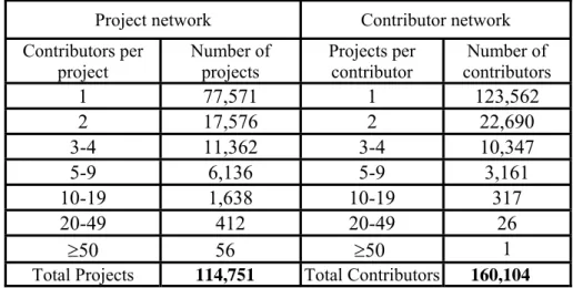
The following table shows the distribution of contributors per project and projects per contributor for the two-mode-network at Sourceforge.net.
Project network Contributor network
Contributors per project Number of projects Projects per contributor Number of contributors 1 77,571 1 123,562 2 17,576 2 22,690 3-4 11,362 3-4 10,347 5-9 6,136 5-9 3,161 10-19 1,638 10-19 317 20-49 412 20-49 26 ≥50 56 ≥50 1
Total Projects 114,751 Total Contributors 160,104
Table 1: The distribution of contributors per project and projects per contributor
Observation 1: (i) Most of the OSS projects are not carried out by large teams of contributors. On average, there are 1.4 contributors per project. More than two-thirds of the projects have only one contributor13 and only 1.8% of the projects have ten or more contributors. (ii) Most of the contributors (90%) participate only in one or two OSS projects.
Table 1 tells an interesting story about the world of OSS projects. Given the excitement generated by open source software, one might imagine a world in which there is an army of contributors who work on many different projects; the reality is different. As Observation 1 indicates 68% of the projects hosted at Sourceforge.net have just a single contributor. An additional 15% of the projects have two contributors. Hence, more than 80 percent of the projects have either one or two contributors. At the other end of the spectrum, there are 1,638 projects with 10-19 contributors and 468 projects with more twenty or more contributors. Table 1 also indicates that 77% of the contributors worked on a single project and more than 90% of
13 While these projects do not provide links between contributors, such contributors who work on multiple projects
9
them worked on just one or two projects. There are a small number of devoted contributors who work on many projects: there are 3,505 contributors who work on five or more projects and 344 contributors worked on ten or more projects. This suggests that the world of open source projects is much less strongly connected than we might have believed.
Since our data is a snap shot taken at a particular date it is possible that projects with one contributor are projects at an early stage of development. There are six levels of development that range from the planning stage to a mature status. There is an additional status reserved for projects that are inactive. Table 2 below provides the distribution of the development status for the single contributor and the multi-contributor projects.
Development status Relative frequency in "single contributor" projects Relative frequency in "multi contributor" projects 1 – Planning 21% 21% 2 - Pre-Alpha 17% 16% 3 – Alpha 18% 17% 4 – Beta 22% 23% 5 – Production/Stable 18% 20% 6 – Mature 1% 2% Inactive 2% 2%
Table 2: Development Status
Observation 2: The distributions of the development status for the single contributor and the multi-contributor projects are similar. Thus the possibility that the single contributor projects are in some way infant projects seems remote.
Of course, in our analysis, we will control for the time for which the project has been in existence, the stage of development and we will examine whether our results are robust to the exclusion of single contributor projects.
2.1 The Network of Contributors:
For the contributor network, there is a link between contributors i and j if they have worked on at least one project in common. The set of contributors can be divided into components such that all of the contributors in a component are connected to one another and there is no sequence of links among contributors in different components. The distribution of the
components is shown in Table 3a. There is a “giant” component, which consists of 55,087 contributors, or approximately 45% of the contributors and many small components as well.
10 Component size (Contributors) Components (sub networks) 55,087 1 196 1 65-128 2 33-64 27 17-32 152 9-16 657 5-8 2,092 3-4 4,810 2 8,287 1 47,787 Table 3a: Distribution of component size
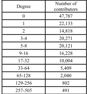
Table 3b: Distribution of Degree
Degree Number of contributors 0 47,787 1 22,133 2 14,818 3-4 20,271 5-8 20,121 9-16 16,228 17-32 10,004 33-64 5,409 65-128 2,040 129-256 802 257-505 491
For every contributor in the network, we can define the degree as the number of links between that contributor and other contributors in the network.14 Table 3b shows the distribution of degree in the contributor network. There are 47,787 contributors who work only in single contributor projects and therefore have a degree of zero. At the other end of the spectrum 491 contributors worked on projects in common with more than 256 other contributors.
Observation 3: Despite the fact that more than 90% of the contributors worked only in one or two projects more than a third of the contributors belong to a giant component of 55,087 connected contributors. The other connected components are relatively small with relatively few contributors.
2.2 The Network of Projects:
In the project network, a node is a project and there is a link between two projects if and only if there are contributors who have contributed to both projects. Table 4a shows the
14 Hence, a contributor who worked on a single project with four other contributors has a
degree of four. Similarly,
a contributor who worked on two projects, each of which had two additional contributors (who only worked on one of the two projects), would also have a contributor degree equal to four.
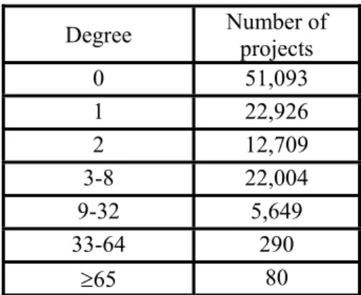
distribution of connected components of the project network. Table 4b shows the distribution of degree for the project network. The degree of a project is the number of other projects with which that project has a link.
Size Connected components 27,246 1 17-27 36 9-16 234 5-8 1,013 3-4 3,419 2 8,020 1 51,093
Degree Number of projects
0 51,093 1 22,926 2 12,709 3-8 22,004 9-32 5,649 33-64 290 ≥65 80
Table 4a: Distribution of component size Table 4b: Distribution of degree Observation 4: (i) The project network has a very special structure. There is one “giant” connected component with 27,246 projects (approximately 24% of the projects at the Sourceforge website) and many very small unconnected components. Remarkably, the second largest connected component has only 27 projects. (ii) Two-thirds of the project have degree less than or equal to one. At the other end of the spectrum, 370 projects have degree greater than thirty-two.
3.
Knowledge Spillovers
Learning is done by individuals. It is possible to distinguish between two types of spillovers: project spillovers and contributor spillovers. In both cases it is the contributors themselves who facilitate the spillovers. But the question is do contributors "learn" from working on a particular project or do they learn from other individuals who collaborate with them. In the former case, we will say that there are "projects spillovers"; in the latter case, there are "contributor spillovers". It is typically very difficult to distinguish between these two types of spillovers. We are able to examine this issue empirically because the unique data set we constructed has detailed information on both projects and contributors.
We start by considering spillovers between projects. Such spillovers can either be direct or indirect. Direct spillovers occur when projects have a common developer who transfers information and knowledge from one project to another. Project spillovers may also be indirect, when knowledge is transferred from one project to another even when the two projects are not directly linked (i.e., they have no common contributor). The indirect spillover route involves a
learning mechanism such that a developer who participates in project X acquires knowledge when he participates in project Y and then employs the knowledge on project X. Another 'project X' developer (who does not work on project Y) then uses that knowledge on project Z. This distinction can be summarized by the following definition.
Definition 1: (i) Direct project spillovers exist whenever there are knowledge spillovers between projects that are directly connected, i.e., they have common contributors. (ii) Indirect project spillovers exist whenever there are knowledge spillovers between projects that are not directly connected, i.e., projects for which there are no common contributors.
An alternative approach would be to assume that contributors accumulate knowledge and there are knowledge spillovers among the contributors. This case involves the contributor network. We again can distinguish between direct and indirect knowledge spillovers allowing contributors to "learn" indirectly from other developers even though they do not work together on the same project.
Definition 2: (i) Direct contributor spillovers exist whenever there are knowledge spillovers between contributors who are directly connected, i.e., they work together on the same project. (ii) Indirect contributor spillovers exist whenever there are knowledge spillovers between contributors who are not directly connected.
Since we do not directly observe spillovers, we will examine the relationship between the network structure and project success in order to identify the relative importance of the different types of knowledge spillovers. We briefly discuss the network measures that are relevant for our analysis. We define these measures in terms of the project network case (the definitions for the contributor network are analogous).
(i). The degree of a project is the number of projects with which it has a direct link or common developers.
(ii). Closeness centrality is defined for every project as the inverse of the sum of all distances between the project and all other projects multiplied by the number of other projects. Intuitively, closeness centrality measures how far each project is from all the other projects in the network. According to this definition closeness centrality lies in the range [0,1]. Formally, for any two nodes i j, ∈N, the distance or degree of separation between them (denotedd i j( , )) is the length
of the geodesic between them where a geodesic is the shortest path between two nodes. Closeness centrality is calculated as:15
(1)
∑
∈ − ≡ N j C j i d N i C ) , ( ) 1 ( ) (Analogously, we can construct the contributor network and derive the network characteristics for each contributor; i.e., the degree and the closeness centrality of each contributor.
We now briefly discuss the relationship between the type of spillovers we have in mind and the network characteristics that we use. We discuss these relationships for the project spillover case, but an analogous structure exists for the contributor spillover case. Assume that all the projects are symmetric except for their position in the network and that the expected success level of each project (without any spillovers) is given by α. Assume further that each project also receives a positive (constant) spillover from all 'connected' projects. Thus, the success level of each project i is α plus β multiplied by the number direct links of each project, i.e.
(2) Si = α + β*Di ,
where Di is the degree of project i in the network and β is the magnitude of the direct spillovers. Now assume that the project also enjoys positive spillovers from projects that are indirectly connected, but that these spillovers are subject to decay. We assume that the greater the distance between the projects in the projects network, the smaller the indirect spillovers. Formally, when the distance between project i and j is denoted as d(i,j), we assume that the expected success of each project is = +
∑
j
i d i j
S α γ / (, ) where γ is the magnitude of the spillovers.16 Using (1) above, project i's success can be rewritten as
(3) ]Si =α +γCc(i))/[N −1 ,
where is the measure of project i's closeness centrality. When (3) holds, the spillovers are fully captured by the closeness measure of each project. Despite this, there are both direct and indirect spillovers.
) (i Cc
15 See Freeman (1979), pp. 225-226 and Wasserman and Faust (1994), pp. 184-185.
13
It is possible that the direct and the indirect spillovers have different impacts. We can capture this by the following (more general) specification:
(4) Si =α+γCc(i)/[N−1]+βDi.
When β =0, there are no additional spillovers from directly connected projects above and beyond those captured by its closeness measure and (4) reduces to (3). Whenβ >0, the spillovers have a 'hyperbolic' structure: there are additional spillovers from directly connected projects.
We will estimate equation (4) and examine if, accounting for the effect of all the control variables (which we will add to the regression), degree and closeness are associated with a larger number of downloads. If the estimated coefficient on closeness is positive and significant, there is evidence for both direct and indirect project spillovers.17 If the estimated coefficient on degree (β) is also positive and significant, there is evidence for a 'hyperbolic' structure with especially strong direct spillovers among connected projects. If γ=0, but β is positive, we have evidence for direct spillovers only, i.e., there are no indirect spillovers. If both γ and β equal zero, there is no evidence for any direct or indirect spillovers.
4. Direct and Indirect Project Spillovers: Empirical analysis
We wish to examine if and what type of knowledge spillovers play a role in the development of OSS projects. We start our empirical analysis by defining a measure of success and different control variables that identify the important characteristics of the OSS projects. Our analysis of the type of knowledge spillovers will be carried out in the following stages. In this section, we will examine the association between project network measures and success. We will then examine the association between contributor network measures and success (Section 5) and then the importance of thick or strong ties among projects (Section 6.)
4.1 Measuring Success/Output in the Project Network
Defining or measuring the success of an open source project is problematic. There are no prices and no ‘sales’. The projects are in the public domain and there is no need to request
14
17 There are possible alternative explanations for a positive association between
degree and closeness and
15
permission or to provide payment for using the OSS. One way to measure project success is to examine the number of times a project has been downloaded. Although this is not always an ideal measure, downloads is a very good measure of success for open source software.18 Unlike downloads of academic papers, users will not typically download a project (and its code) unless it will be useful to them for some task.19
Every month, the Sourceforge.net staff chooses a “project of the month.” Although we do not know the exact criteria that are employed in choosing the “project of the month,” these projects are likely to be very “successful.” We obtained data on the "project of the month" for the forty-two month period ending in June 2006. The “project of the month” projects have an especially large number of downloads.20 “Project of the month” projects are typically in advanced stages (stages 4,5, and 6); thirty-eight of the forty-two projects of the month projects are either in stage 4, stage 5, or stage 6. The thirty-eight “project of the month” projects in advance stages had on average 6,028,560 downloads, versus 30,206 downloads (on average) for the other 35,821 projects in advanced stages. The median number of downloads for “project of the month” projects in advance stages was 1,154,469 versus 483 for other projects in advance stages. This suggests that the number of project downloads is an attractive measure of use and value.
There are several different download measures that we could use: (i) the total number of downloads since the project was initiated at Sourceforge.net (ii) the maximum number of downloads in any month, and (iii) the number of recent downloads. The correlation among these download measures is, however, quite high. Since it contains the most information, we chose to use the total number of downloads in our analysis. Henceforth, when we refer to downloads, we mean the total number of downloads and denote downloads as the total number of downloads for the forty-two month period for which we have data. We further define ldownloads ≡
ln(1+downloads), where “ln” means the natural logarithm.
18 Downloads are also often used in order to measure the impact of academic papers and articles on the web. The
Social Science Research Network, for example, provides information on the number of downloads for the papers on its website.
19 In some cases, the number of downloads is small relative to the number of contributors. In such cases, the
number of downloads may be affected by the fact that developers may need to download the code of the project when working on the project. When we restrict our analysis to projects with more than 200 downloads, and a download/contributor ratio of at least ten-to-one (so that the number of downloads is at least an order of magnitude larger than the number of developers), our results remain qualitatively unchanged: hence our results are robust to the possibility of 'developer' downloads. See section 4.4.1.
16
4.2 Network and Control Variables (Project Characteristics)
For our empirical analysis, we employ the project network variables ldegree = ln(1+degree) and lcloseness = ln(0.05+closeness),21 where degree and closeness were defined in section 3. In addition to downloads and the network variables, we have data for a group of control variables that includes the amount of time that the project has been in existence, the stage of development, the number of operating systems for which the program was written, the number of languages in which the program is written, as well as several other control variables:
• The variable years_since is the number of years that have elapsed since the project first appeared at Sourceforge: lyears_since=ln(years_since).
• The variable cpp is the number of contributors that participated in the project: lcpp=ln(cpp)
• The dummy variable ds_j refers to the stage where j ranges from one to six. There is an additional stage, denoted inactive, which means the project is no longer active. See Table 2. A few of the projects are considered to be in multiple stages. Hence, for a particular project, it is possible that both ds_3 and ds_4 could be equal to one.
• The variable count_trans is the number of languages in which the project appears including English. Virtually all of the projects (95%) are available in English. The other popular languages include German (5% of the projects), French (4%), and Spanish (3%).
lcount_trans=ln(count_trans)
• The variable count_op_sy is the number of operating systems (i.e., formats) in which the project is compatible. Some of the projects are available for several operating systems. The main operating systems in which the projects were written include Windows (32% of the projects), Posix (26% of the Projects), and Linux (21% of the Projects. lcount_op_sy=ln(count_op_sy)
• The variable count_topics is the number of topics included in the project description. Popular topics include the Internet (16% of the projects), software development (14%), communications software (11%), and games & entertainment software (10%). lcount_topics=ln(count_topics)
• The variable count_aud is the number of main audiences for which the project was intended. The main audiences are developers (35% of the projects), end users (30% of the projects), and system administrators (13% of the projects). Some of the products are intended for multiple ‘main audiences’ while other projects are not intended for these main audiences, but rather just for niche audiences, i.e., just for a particular industry (i.e.,
21 The reason we add such a small number is because the mean value of
17
telecommunications) or just for very sophisticated end users. lcount_aud = ln(1+count_aud)
Clearly, there are different ways to construct these variables. For example, we could have simply counted the key operating systems, or used dummy variables for these operating systems. Similarly, we could have defined dummy variables for ‘main audiences’ or we could have added up the number of main audiences together with the number of niche audiences. We chose the definitions that seemed most natural. Our main results regarding the number of contributors and the network variables are robust to alternative definitions of these control variables.22
4.3 Empirical Results
We estimate a simple log/log model of the form ldownloadsi = α + βNi + γCi + εi, where the subscript i refers to the project. Ni is the natural logarithm of the “network variables” and Ci is the natural logarithm of the control variables.23 For binary ({0,1}) variables, we, of course do not employ logarithms; εi is a random error term.
We have data on 114,450 observations for all of the network variables as well as on years_since.24 However, data on the stage of development and the count variables are incomplete; data on all of the control variables are available only for 66,511 projects. Since there is no selection issue,25 we use only the data on the 66,511 projects for which we have complete information. We use information from all the projects to construct the network variables that are included in the database. We first conduct an analysis using these projects and examine the association between degree (and the control variables) and success. We then examine the giant component in detail (18,697 projects for which there is complete information), which enables us to include closeness in the analysis.26
22 Contributor effort is not observable. As we discussed in the introduction, the main reward to OSS contributors is
being included in the list of contributors. Thus the incentive they have is to provide the sufficient effort to accomplish this status. Hence, effort is not likely correlated with network measures or the control variables – and hence, the absence of data on effort does not bias our results.
23 The relationship between the number of contributors and
downloads is likely non-linear: additional contributors
are likely associated with a larger number of downloads, but the marginal effect of each additional contributor declines as the number of contributors increases. The same is likely true for the relationship between the network variables and downloads as well. This suggests that a "log/log" model is appropriate. We examine alternative functional forms in section 4.4.2. In that section, we indeed show find that the log/log specification has a higher adjusted R-squared that both the log/linear and linear/linear specifications.
24 There are 114,751 total projects, but we are missing data on downloads for a small number of them (301). 25 See Griliches (1986) and Greene (1993).
26 The values of
degree and closeness centrality are calculated using the software program Pajek, which is a
18
The effect of degree (as well as other effects) may depend on whether the project is in the giant component or not; we therefore introduce the variable "giant_comp" which is a dummy variable that takes on the value one if the project is in the giant component, and takes on the value zero otherwise. In order to allow for the possibility that the association between degree and downloads and between the number of contributors and downloads depends of whether the project is inside or outside of the giant component, we also include the following interaction variables in the analysis:
• lgiant_degree = ldegree*giant_comp, • lgiant_cpp = lcpp*giant_comp,
By including the interaction variables, we allow for the possibility that there will be different download “elasticities” for projects in and projects outside of the giant component.27
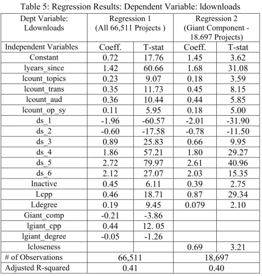
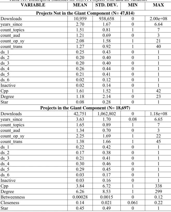
Descriptive statistics of the variables are shown in Table A1 in the appendix. Table A1 shows that projects in the giant component have on average many more downloads than projects outside of the giant component (42,751 vs. 10,959). Further, projects in the giant component are on average (i) older than projects outside of the giant component (3.63 years vs. 2.70 years), (ii) have more contributors (3.84 vs. 1.61), and (iii) have a larger degree (6.26 vs. 1.18).28 The results of a regression with all 66,511 observations are shown in the first column of Table 5. The effect of the number of contributors: The estimated coefficients show that the association between downloads and the number of contributors is positive – projects with more contributors have a greater number of downloads. For projects outside of the giant component, the estimated “contributor” elasticity is 0.46. This effect is statistically significant. The estimated “contributor” elasticity is virtually twice as large for projects in the giant component: 0.90 (0.46+0.44). The difference in the estimated “contributor” elasticity between projects in the giant component and projects outside of the giant component is statistically significant: additional contributors are associated with greater increases in output for projects in the giant component than in the non-connected component. This result obtains despite the fact that there are many more contributors (on average) for projects in the giant component (3.84 vs. 1.61).
27 The addition of different slopes for the control variables based on whether the project was inside or outside of the
giant component has no effect on the main results regarding the number of contributors and the degree of the
project.
28 Correlations among the network centrality variables in the giant component are shown in Table A2 in the
19
The effect of project's degree: The association between the degree of the project and the number of downloads, is positive and statistically significant both for projects inside the giant component and for projects outside of the giant component. For projects outside of the giant component, the degree elasticity is 0.19, while the degree elasticity for projects in the giant component is 0.14. Both of these magnitudes are statistically significant from zero; the difference in the magnitudes is not significantly different from zero.
The effect of the control variables: The estimated coefficient of lyears_since is positive (1.42) and statistically significant. Projects that have been active longer have more downloads, and the estimated coefficient suggests that a doubling of the time a project has been active is associated with 142% more downloads. The estimated coefficients on the stage variables have the expected signs. By and large, projects that are in more advanced stages are associated with more downloads. Similarly, projects written for several operating systems, projects available in more languages, projects written for more main audiences, and projects that span more topics are associated with more downloads as well.
Observation 5: (i) Projects in the giant component have on average (four times) more downloads than projects outside of the giant component. (ii) Projects with more contributors have a greater number of downloads and this effect is stronger in the giant component. (iii) The association between the degree of the project and the number of downloads, is positive and statistically significant (both inside and outside the giant component).
From Observation 5 we can conclude that the network architecture does affect the number of downloads which suggests that there are knowledge spillovers among the projects.
Table 5: Regression Results: Dependent Variable: ldownloads Dept Variable: Ldownloads Regression 1 (All 66,511 Projects ) Regression 2 (Giant Component - 18.697 Projects)
Independent Variables Coeff. T-stat Coeff. T-stat
Constant 0.72 17.76 1.45 3.62 lyears_since 1.42 60.66 1.68 31.08 lcount_topics 0.23 9.07 0.18 3.59 lcount_trans 0.35 11.73 0.45 8.15 lcount_aud 0.36 10.44 0.44 5.85 lcount_op_sy 0.11 5.95 0.18 5.00 ds_1 -1.96 -60.57 -2.01 -31.90 ds_2 -0.60 -17.58 -0.78 -11.50 ds_3 0.89 25.83 0.66 9.95 ds_4 1.86 57.21 1.80 29.27 ds_5 2.72 79.97 2.61 40.96 ds_6 2.12 27.07 2.03 15.35 Inactive 0.45 6.11 0.39 2.75 Lcpp 0.46 18.71 0.87 29.34 Ldegree 0.19 9.45 0.079 2.10 Giant_comp -0.21 -3.86 lgiant_cpp 0.44 12. 05 lgiant_degree -0.05 -1.26 lcloseness 0.69 3.21 # of Observations 66,511 18,697 Adjusted R-squared 0.41 0.40
Our next step is to introduce the variable lcloseness into the regression (see the second regression in Table 5). Since closeness is only comparable across linked networks, this regression is done for the giant component only (18,697 observations). Note that in the new regression the estimated contributor elasticity (0.87, t=16.71) and the estimated coefficient on lyears_since (1.68, t=31.08) are again positive and statistically significant. The estimated coefficients on the stage and count variables again have the expected signs and are qualitatively similar to those in the first regression in Table 5.
This regression also shows that the estimated closeness elasticity (0.69, t=3.21) is statistically significant. Controlling for closeness, there is still a positive association between the number of downloads and the degree of the project. The estimated degree elasticity (0.079, t=2.10) is also statistically significant in this regression.
21
Observation 6: Closeness is positively and significantly associated with higher downloads. This suggests that indirect spillovers are important.
The second regression in Table 5 indicates that the estimated coefficient on degree is also positive and significant. This suggests that there are 'hyperbolic' direct spillovers as well. We now will conduct several robustness tests in order to examine whether these results are robust.
4.4 Robustness Analysis
In this section, we will examine whether the results in the second regression in Table 5 are robust by examining established projects only, projects with more than one contributor, and projects with a relatively large number of downloads. We then examine the robustness of the results to functional form, to possible endogeneities, and to including an additional network centrality measure. We conclude this section by examining alternative interpretations of the results.
4.4.1 Established projects, more than one contributor, and a large number of downloads Nascent projects may not have reached a steady-state number of contributors. Personnel additions are probably more likely for relatively new products. Here we examine whether our results are robust to using only established projects in the analysis. We also restrict the analysis to projects in existence for at least two years. For similar reasons, we also restrict the analysis here to projects with more than one contributor. (We focus henceforth on the second regression in Table 5 because this regression includes degree and closeness.)
In some cases, the number of downloads is small relative to the number of contributors. In such cases, the number of downloads may be affected by the fact that developers may need to download the code of the project when working on the project. Hence, we also restrict our analysis to projects with more than 200 downloads, and a download/contributor ratio of at least ten-to-one (so that the number of downloads is at least an order of magnitude larger than the number of developers).
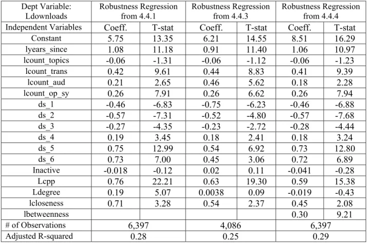
When we include all of the above three robustness "restrictions" together (projects with more than one contributor, projects in existence for more than two years, projects with more than 200 downloads, and a download/contributor ratio of at least ten-to-one), we are left with 6,397 observations. We again find that the estimated contributor elasticity (0.76, t=22.21), the estimated closeness elasticity (0.71, t=3.28), and the estimated degree elasticity, (0.19, t=5.07)
22
are positive and statistically significant. The robustness analysis thus suggests that the results regarding the contributor elasticity, closeness and degree are robust to all of these changes. These results are shown in the first regression in Table A3 in the appendix.29
4.4.2 Robustness to Functional Form
When we run a log/linear regression (the dependent variable remains in logarithms, but the independent variables are in levels), we have the following results: the estimated coefficient on closeness is positive and statistically significant both for a regression with all observations in the giant component, as well as for a regression (6,397 observations) with all three robustness restrictions discussed above in section 4.4.1. The estimated coefficient on degree is insignificant in a regression with all observations in the giant component; it is positive and statistically significant in a regression with all three robustness restrictions from section 4.4.1.
When we run a linear/linear regression (both the dependent variable and the independent variables are in levels), rather than a log/log regression, the estimated coefficient on closeness is still positive and statistically significant. The estimated coefficient on degree is positive, but no longer statistically significant. This result holds both for a regression with all observations in the giant component (18,697), as well as for a regression (6,397 observations) with all three robustness restrictions from section 4.4.1.30
We can thus conclude that the positive and statistically significant results regarding closeness are robust to functional form. The results on degree are not completely robust to functional form.
4.4.3 Potential Endogeneities
Degree could be endogenous in our data set. Here, the interpretation would be that developers may want to be associated with more successful projects. This would make degree endogenous. (This is sometimes referred to the 'chicken' vs. 'egg' issue.)
Closeness could also be endogenous under the following scenario: developers may want to work on a particular project so that a developer on that project can "introduce" them to a
29 The same qualitative results are obtained when we examine these three robust restrictions separately. The
estimated contributor elasticity remains positive and statistically significant in all specifications. Since our focus is on degree and closeness, we do not discuss the estimated contributor elasticity in the analysis that follows.
30 The linear/linear specification has a very low adjusted R-squared (0.04). In contrast, the log/linear specification
has an adjusted R-squared of 0.25; the log/log specification (regression #1 in Table A3) has an adjusted R-squared of 0.28.
23
developer (on another project) whom they would like to meet. Since our network is a fairly thin one (many projects and relatively few developers) and that the average project in our dataset has less than four contributors to a project in the giant component, it is unlikely that this indirect contact mechanism would play any role. It would likely be much easier and much more effective to simply contact the programmer directly. Nevertheless, we wish to address this potential endogeneity as well
With the exception of Calvo-Armengol, Patacchini, and Zenou (CPZ, 2008), we are not aware of any empirical papers in the social network literature that estimate a structural model and (hence) are able to econometrically deal with the endogeneity issue by using instruments. Unfortunately, neither the CPZ (2008) nor other theoretical models (like König et al., 2008) are appropriate for our setting. Even if we could develop a structural model, it would likely depend on variables like effort or marginal cost that are not observable.
Hence, we must address the potential endogeneity of degree and closeness in another way. One way to address this issue is indeed to only consider relatively young projects. The 'joining popular projects' effect is likely to be less of a factor for relatively young projects. When we run a regression with projects less than 3.63 years old (the mean age of the projects in the giant component), with more than 200 downloads and a download/contributor ratio greater than 10, we find the following:31 The estimated coefficient on closeness remains positive and statistically significant (0.54, t=2.37), while the estimated coefficient on degree (0.0038, t=0.09) is not statistically significant. (These results appear in the second regression in Table A3 in the Appendix.)
This suggests that degree is indeed potentially endogenous. Nevertheless, the estimated coefficient on closeness is virtually unchanged. These results suggests that closeness is not endogenous and that, despite the potential endogeneity of degree, the results for closeness remain qualitatively unchanged. Our main conclusion, that there are both direct and indirect spillovers, holds despite the potential endogeneity of degree.
4.4.4 The flow of Information: Betweenness Centrality
In this section, we consider another centrality measure -- betweenness centrality – and we examine whether our results are robust to its inclusion. Before we define betweenness centrality,
31 We did include projects with a single contributor here because they are important when examining 'young'
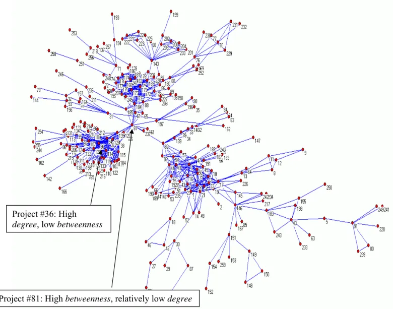
we will illustrate this measure by using the (thick) project network shown in Figure 2 in the Appendix. We can see that this network has an interesting structure. There are three clusters or groups of highly connected projects.32 The three clusters remain connected as part of one component only because project 81 is connected to all these three groups. Project 81 has a relatively small degree, but its position in the network is unique and central. This position is relevant for an additional type of knowledge spillover. Assume for example that the three groups in Figure 2 describe a friendship network among people. Moreover assume that each cluster in this network is a group of friends that are similar in their backgrounds and preferences. Suppose that the knowledge transmitted in this network is about the quality of a restaurant or a movie. In this case the information received from members of the same group would be more valuable than information received from members of other groups. On the other hand, there are research settings where ideas come from groups of researchers who think and solve problems in different ways. It is possible that in such an environment the more valuable knowledge spillovers come from outside of the research group's inner core. In these cases, the position of project 81 (Figure 2), which is linked to several different clusters of projects, may benefit from valuable knowledge spillovers from the different clusters of projects.
We capture this effect by introducing betweenness centrality into our empirical analysis. Betweenness centrality is defined as the proportion of all geodesics between pairs of other nodes that include this node.33 Betweenness captures the notion that a node is considered "central" if it serves as a valuable juncture between other nodes. Project 81 in Figure 1 indeed has relatively high betweenness. Formally, the betweenness of a node is given by i
(5) { , } ( ) ( ) (# 1)(# 2) 2 j k jk jk i j k N B i C i N N γ γ < ∉ ⊆ ⎡⎣ ⎤⎦ ≡ − −
∑
where γjk is the number of distinct geodesics between the nodes j and which are distinct from , and
k
i γjk( )i is the number of such geodesics which include i.34 When we add betweenness to the analysis, and run a regression (6,397 observations) with all three robustness restrictions from section 4.4.1, we find that the estimated coefficient on degree is insignificant, while the estimated coefficient on closeness remains positive and statistically significant
32 Each has some periphery networks that are connected only to one particular group. 33 See Freeman (1979), pp. 230-231 and Wasserman and Faust (1994), pp. 189-190.
24
34 The denominator of (1) is the maximum possible value for the numerator, and thus standardizes the measure in
25
(coeff=0.45, t=2.08.) This again suggests that our results on closeness are again robust. The estimated coefficient on betweenness is positive and statistically significant, suggesting the possibility of an additional type of knowledge spillover. (These results appear in the third regression in Table A3 in the Appendix.)
Robustness results in sections 4.4.1-4.4.4 show that the estimated coefficient on closeness remains positive and statistically significant in all 'robustness' specifications, while degree becomes insignificant in several instances. Note that a positive coefficient on closeness provides evidence for both direct and indirect spillovers. Since the coefficient on degree becomes insignificant in several robustness regressions in sections 4.4.1-4.4.4, we do not find convincing evidence for 'hyperbolic' direct spillovers.
Observation 7: Both direct and indirect spillovers are important. Closeness is positively and significantly associated with higher downloads. However, we do not find convincing evidence for hyperbolic direct spillovers as, controlling for closeness, there is not always a positive association between the degree of the project and number of downloads.
4.4.5 Alternative Interpretations of the Results
Positive correlations are, of course, not sufficient for identifying a knowledge spillover. Indeed, the interpretation of a direct knowledge spillover would be problematic if there were only a few highly productive developers and these productive developers signed up for many projects and also caused their projects to have high downloads. In such a case, degree would be significant in the regression, yet there would be no knowledge spillover.
We went back and excluded projects that had developers who worked on five or more projects (i.e., 'star' contributors). In this new robustness regression, we included the robustness restrictions from section 4.4.1 (more than one contributor, projects that were at least two years old, projects with more than 200 downloads and a download/contributor ratio greater than 10.) We had 2,917 observations in this regression. The summary of the regression results (for the network variables) is as follows: Both the estimated coefficient on closeness (0.77, t=2.51), and the estimated coefficient on degree (0.38, t=4.54) remain positive and statistically significant.
There is also an alternative explanation (i.e., non-spillover story) regarding the positive correlation between closeness and success: if highly productive developers work together (a few to a project), their projects will be high in 'connectedness' since they will be linked to other projects characterized by many links even if there is no spillover. While this story is plausible in a small, relatively tightly connected network, it is unlikely in our network, which is huge and
26
fairly thinly connected (see Table 1.) This suggests that the interpretation of degree and closeness as knowledge spillovers is reasonable in our case.
5. Contributor
Network
Characteristics and Project Success
Until this point, we focused on project network characteristics and the way they were associated with the success of the projects. Our next step is to focus on the contributor network characteristics and to examine their relation to project success.
5.1 The effect of contributor characteristics.
We construct the contributor network and derive the network characteristics for each contributor. In order to examine the relationship between these characteristics and project success, we need to look at the group of contributors who participate in each project and define measures that capture the network characteristics of these contributors. For each project we form a list of contributors and construct the following variables:35
(i) Average degree of the contributors in a project.
(ii) The average closeness centrality of the contributors to a project.
The above variables differ respectively from the degree of a project and the closeness centrality of a project. For example, consider project A with two contributors (denoted I and II), each of whom works on one other project. This means that project A has a (project) degree equal to two. Further suppose that contributor "I" also works on project B, and that there are three other distinct contributors on project B. Similarly, suppose that contributor II also works on project C, and that there are again three additional distinct contributors on project C. The "contributor" degree of contributor I equals four (since he/she participates with four other contributors in two different open source projects). Similarly, the contributor degree of "II" is four as well. Hence, the average contributor degree of project A is four.
While the degree of the project and the average degree of the contributors to a project are relatively highly correlated in our data set (0.44),36 there is virtually no correlation between the closeness centrality of a project and the average closeness centrality of its contributors (0.03).
35 Our results are robust to employing the maximum
degree and maximum closeness centrality of the contributors
on a project rather than the average degree and closeness centrality of the contributors on a project
27
We first ran a regression similar to the second regression in Table 5 with the two contributor network variables instead of the two project network variables. Neither the average closeness centrality of the contributors to a project (coefficient = 0.12, t = 1.59) nor the average degree of the contributors on a project (-0.019, t = -0.72) are statistically significant. When we include both the project and contributor centrality variables in the regression, we find that project centrality measures (degree and closeness) are again highly associated with success, while the contributor centrality variables are not associated with project success.
Observation 8: Our analysis indicates that with respect to OSS software development it is the project spillovers which are important and not the contributor spillovers. Specifically, direct and indirect project spillovers are associated with project success while knowledge spillovers between individual contributors are not associated with project success.
Our analysis examined two types of spillovers; spillovers between projects and spillovers between individuals. In both cases it is the contributors themselves who facilitate the spillovers. But the question is do they "learn" from working in a particular project or do they learn from other individuals who collaborate with them. Observation 8 states an interesting result: in the world of OSS projects, spillovers occur between projects and not between participants.
5.2 The "Star" Effect
Some of the contributors in our data set work in many projects. The question is if these individuals have special talents or ability that make a significant contribution to the projects in which they participate. We define a "star" as a contributor who worked on five or more projects. Clearly having a "star" contributor gives a project more connections with other projects. Indeed we find that stars are much common in projects that are in the giant component. Specifically, 45% of the projects in the giant component have at least one star while only 8% of the projects outside of the giant component do not have a star. An interesting question is if having a "star" in the team of developers has an effect on the success of a project.
To examine this, we add a dummy variable (denoted star) -- which takes on the value one if the project has at least one star and takes on the value zero otherwise -- to the second regression in Table 5. The estimated "star" contributor is negative (-0.14, t=-1.94). Since degree and star are highly correlated, one possibility is that any positive effect associated with a 'star' is picked up by degree.37
37 The estimated coefficient on
28
Observation 9: After controlling for network centrality measures, 'star' programmers do not make any significant contribution to project success. That is, 'star' programmers do not make a difference beyond that captured by changes in the network measures of the projects in which they participate.
Note that our above conclusion is with respect to having a star working for the project and holding the degree and the structure of the network fixed. Clearly, when a star contributor chooses to work for a certain project he changes the network structure and in particular the network characteristics of the project for which he works. Hence, the above observation suggests that any additional contributions made by star contributors are fully taken into account by the change in the network measures.
6.
The Importance of Strong Ties
So far we defined two projects to be linked if there was at least one contributor in common between them. But the potential of spillovers between projects may depend also on the number of contributors who participated in both projects. To capture this effect we change the definition of a link and focus only on "strong" (or thick) links. Two projects are ‘strongly’ linked if they have at least two contributors in common. That is, we define a new network in which the nodes are still projects, but the links are only 'strong' (thick) links.
Redefining the network has a dramatic effect on it structure. Previously in a network in which one contributor in common was sufficient for a link, there was a giant component of 27,246 projects. In the strongly connected network, the largest component of strongly connected projects consists of only 259 projects. There are four other smaller strongly connected components with between 50-75 projects. No other components have more than 27 projects.38
A comparison between projects in the (i) large strongly connected component, (ii) the four smaller strongly connected components, (iii) and other projects in the giant component is presented below in Table 6.39
38 Figure 2 in the Appendix shows the structure of the largest component in the "strongly connected" network. 39 The same qualitative result obtains if we restrict the analysis to projects in stages 4-6. In such a case, the medium
(mean) number of downloads are respectively: 11,230 (155,428) for projects in the largest strongly-connected component, 2,896 (85,204) for projects the four smaller strongly connected components and 1,419 (73,532) for projects in other projects in the giant component.