ASEAN-5 Macroeconomic Forecasting Using a GVAR Model

(1)

ASEAN-5 Macroeconomic Forecasting Using a GVAR Model

Fei Han and Thiam Hee Ng

No. 76 |

March

2011

ADB Working Paper Series on

Regional Economic Integration

(2)

(3)

ADB Working Paper Series on Regional Economic Integration

ASEAN-5* Macroeconomic Forecasting Using

_a

GVAR Model

Fei Han+_{and Thiam Hee Ng}++

No. 76 March 2011

*ASEAN-5 in this paper refers to the original five ASEAN members: Indonesia, Malaysia, Philippines, Singapore, and Thailand.

The authors would like to thank Lei Lei Song and Renato E. Reside for their helpful suggestions and valuable comments. The authors also wish to give special thanks to OREI ADB consultants Julie Ann Basconcillo for her help in computing the trade weights, and Marthe Hinojales for helping apply StataCorp LP’s STATA software. Any errors are our own.

+_{Fei Han is an intern, Office of Regional Economic} Integration, Asian Development Bank, and a PhD Candidate, University of California, Berkeley. email: [email protected]

++_{Thiam Hee Ng is Economist, Office of Regional} Economic Integration, Asian Development Bank, 6 ADB Avenue, Mandaluyong City, 1550 Metro Manila, Philippines. Tel: +63 2 632 4522, Fax: +63 2 636 2342, email: [email protected]

(4)

The ADB Working Paper Series on Regional Economic Integration focuses on topics relating to regional cooperation and integration in the areas of infrastructure and software, trade and investment, money and finance, and regional public goods. The Series is a quick-disseminating, informal publication that seeks to provide information, generate discussion, and elicit comments. Working papers published under this Series may subsequently be published elsewhere.

Disclaimer:

The views expressed in this paper are those of the authors and do not necessarily reflect the views and policies of the Asian Development Bank (ADB) or its Board of Governors or the governments they represent. ADB does not guarantee the accuracy of the data included in this publication and accepts no responsibility for any consequence of their use.

By making any designation of or reference to a particular territory or geographic area, or by using the term “country” in this document, ADB does not intend to make any judgments as to the legal or other status of any territory or area.

Unless otherwise noted, $ refers to US dollars.

(5)

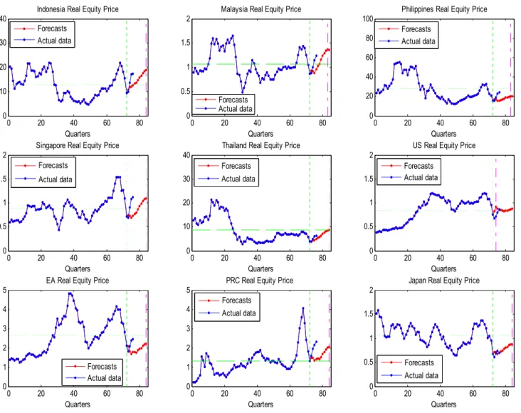
1. One Quarter Ahead Forecasts for Real GDP Growth 19 2. One Quarter Ahead Forecasts for Inflation 20 3. One Quarter Ahead Forecasts for Short-Term Interest Rate 21 4. One Quarter Ahead Forecasts for Real Exchange Rate 22 5. One Quarter Ahead Forecasts for Real Equity Prices 23 6. Generalized Impulse Responses of a Negative Unit (1 s.e.)

Shock to US Real Equity Prices 24

7. Generalized Impulse Responses of a Negative Unit (1 s.e.)

Shock to US Real Equity Prices 25

8. Generalized Impulse Responses of a Positive Unit (1 s.e.) Shock to World Commodity Prices in the US Model 26 9. Generalized Impulse Responses of a Positive Unit (1 s.e.)

Shock to World Commodity Prices in the US Model (cont.) 27 10. Generalized Impulse Responses of a Positive Unit (1 s.e.)

to US Short-Term Interest Rates 28 11. Generalized Impulse Responses of a Positive Unit (1 s.e.)

(7)

Abstract

This paper examines and evaluates macroeconomic forecasts for the original ASEAN-5 members in the context of a global vector autoregressive (GVAR) model covering 20 countries, grouped into nine countries/regions. After estimating the GVAR model, we generate 12 one-quarter-ahead forecasts for the next quarter including real GDP, inflation, short-term interest rates, real exchange rates, and real equity prices over the period 2009Q1–2011Q4,**_{with four out-of-sample forecasts over the period 2009Q1–2009Q4.} Forecast evaluation results based on the panel Diebold-Mariano (DM) tests show the GVAR forecasts tend to outperform forecasts based on the benchmark country-specific models, especially for short-term interest rates and real equity prices, emphasizing the interdependencies in the global financial market.

Keywords: Macroeconomic Forecasting, Global vector autoregressive model (GVAR),

Southeast Asia

JEL Classification: E37, F47

(8)

(9)

ASEAN-5 Macroeconomic Forecasting Using a GVAR Model | 1

1. Introduction

There are various time series models for macroeconomic forecasting, which can be generally classified into two different approaches: structural approach and reduced-form approach. Although the structural approach is model-oriented and embeds more economic structures, it usually requires building a complex economic model with multiple parameters. As a result, it is more sensitive parameter estimates and underlying assumptions about the economy relative to the reduced-form approach. It is also computationally more intense and difficult to implement in practice—especially when doing macroeconomic forecasting for more than one country. On the other hand, the reduced-form approach is usually more data-oriented and does not incorporate many economic structures, but it is easier to implement with its smaller computational requirements.

Most time series models belong to the reduced-form approach. For univariate forecasting, autoregressive moving variable (ARMA) and autoregressive integrated moving variable (ARIMA) models are frequently used in literature for stationary and nonstationary time series, respectively; autoregressive conditional heteroskedasticity/generalized autoregressive conditional heteroskedasticity (ARCH/GARCH) models are useful to model time series with time-varying conditional variance—demonstrating their power for estimation and forecasting in finance. For multivariate stationary time series, the vector autoregressive (VAR) model, a generalization of the univariate autoregressive model, is able to capture the evolution and interdependencies among multiple time series. Sim (1980) proposed a Cholesky decomposition method to solve the well-known identification problem of the original VAR system. However, this VAR approach has been criticized as being devoid of any economic content.

Therefore, many economists and econometricians have been trying to come up with new techniques to incorporate the pros of the structural approach into VAR. Sims (1986) and Bernanke (1986) proposed imposing economic restrictions on the regression innovations—known as the Structural Vector Autoregression (SVAR) model. However, one needs to impose too many economic restrictions—(n2_-_n_{)/2 restrictions—in an} n-variable VAR in order to achieve identification, which is quite difficult and sometimes impossible when there is more than one country in the sample.

Besides these technical issues, another important feature of macroeconomic forecasting we need to consider is the increased globalization and interdependency of the world economy. This has important consequences for conducting monetary and financial policies by central bankers and risk management by commercial bankers. The main motivation for this paper is to forecast the main macroeconomic variables for ASEAN-5. Since these five countries all mid-sized, open economies and are highly affected by other world economic powers such as the United States (US), it is necessary for us to take into account these external impacts.

In this paper we employ the global vector autoregressive (GVAR) model originally introduced by Pesaran, Schuermann, and Weiner (2004) and further developed by Dees et al. (2007) and Pesaran et al. (2009) to develop a macroeconomic forecasting model for the ASEAN-5 countries. The advantage of the GVAR model is that it not only incorporates

(10)

economic structures and global interdependencies of the world economy into the VAR model, but also avoids the identification problem in VAR. Furthermore, there are major differences in the cross-country correlations of various real variables. For instance, equity returns are much more closely correlated across countries than real GDP growth and inflation. This suggests that different channels of transmission should be considered. The GVAR approach allows us to model these different types of links directly, using trade-weighted observable macroeconomic aggregates and financial variables.

The plan of the paper is as follows: Section 2 presents the GVAR model, its assumptions, and the estimation strategy. Section 3 describes the data used. Section 4 presents tests for two assumptions of GVAR, and contemporaneous effects of foreign variables on their domestic counterparts. Section 5 presents the forecasting results and evaluation. Section 6 derives generalized impulse response functions for the analysis of country-specific shocks. Section 7 offers some concluding remarks.

2. The GVAR Model

There are two steps in constructing a GVAR model: the country-specific models and the global VAR. In this section, we provide an overview of the GVAR framework describe the country-specific models and explain how the global VAR is constructed. We can thus ensure that the forecasts obtained for different countries are internally coherent within the GVAR modeling framework.

**2.1. Country-Specific VARX* Models**

The country-specific model is a VARX* model1_{for each individual country/region. The} endogenous variables in most country-specific models include the following core variables:

(

)

(

)

(

)

(

)

(

)

(

)

( )

, 1

ln

0.25ln 1

100 ln

it it it it it i t it it it it it it S it it W W t t

y

GDP CPI

CPI

e

E CPI

q

EQ CPI

r

R

p

P

π

₋

=

−

=

+

=

(11)

where:

GDPit = nominal gross domestic product of country i during period t (in local currency),

CPIit = consumer price index for country i at time t (with the base year at 100),

Eit = exchange rate of country i currency at time t in US dollars,

EQit = nominal equity price index,

S it

R = nominal short-term interest rate per annum, in percent, W

t

P = world commodity price index.

The typical maturity of short-term interest rates is 3 months. Full details of data sources are given in the Appendix. The US is indexed as country 0, and the exchange rate of the US—E0t—is taken to be 1. In the country-specific model for each country/region other

than the US, the endogenous variables are

(

y

_it

,

π

_it

, , ,

r e q

_it _it _it

)

; while for the US model, the endogenous variables are

(

₀ , ₀ , ,₀ ₀ , W

)

t t t t t

y

π

r q p . Note that the endogeneity of the world commodity price in the US model reflects the large size of the US economy (it alone accounts for about one-quarter of world output in nominal terms). The real equity price is also included as an endogenous variable to capture the financial market shocks.2

The (weak) exogenous variables in the country-specific VARX* models are trade-weighted foreign core macro-variables (denoted by an “*”). In most country-specific models, foreign variables are constructed as

0 0 0 0 0

,

N N N it ij jt it ij jt it ij jt j j j N N it ij jt it ij jt j j

y

w y

w

e

w e

q

w q

r

w r

π

∗ ∗ ∗ = = = ∗ ∗ = =

=

∑

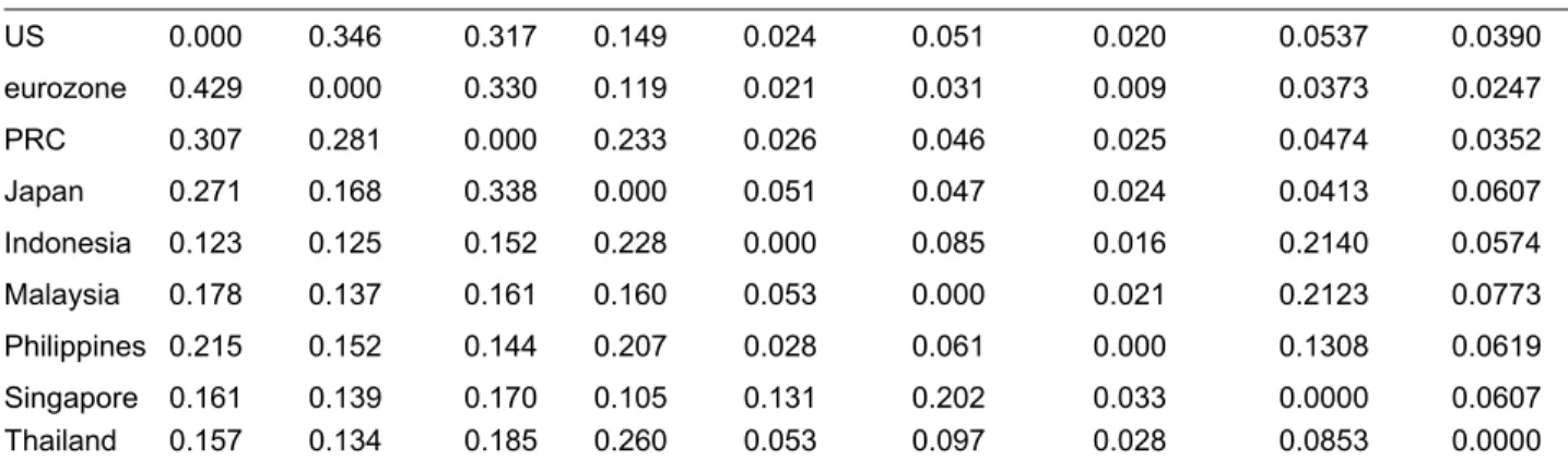
The weights wij for i,j = 0,1,…,N3 are trade weights between country i and country j

computed using the simple average of monthly total trade of a country/region during the 2007–2009 period. wii is 0 for any country i. Table 1 shows the trade weights within all

countries examined here. We use the exogenous variables in Dees et al (2007). In the country-specific model for each country or regional economy other than the US, the exogenous variables are

(

, , , , W

)

it it it it t

y∗

π

∗ r q p∗ ∗ _{, while for the US model, the exogenous}

variables are

(

y₀t,

π

₀t,e₀t

)

∗ ∗ ∗ _.4_{The inclusion of only three foreign variables in the US} model reflects the importance of US financial markets within the global financial system. Once the variables to be included in the different country models are specified, we begin

2_{See Dees et al (2007) for choice of variables. The long-term interest rate is not included in this paper as}

an endogenous variable as data for ASEAN-5 are unavailable.

3 _N

= 8, which is the number of countries/regions minus the US used in this paper.

4_{Although foreign inflation does not pass the exogeneity test within our sample period, it remains included}

(12)

the modeling following the assumptions in Dees et al. (2007)—that all the country-specific variables are I(1), the country-specific exogenous variables are weakly exogenous, and that the parameters of the country-specific models remain stable over time. These two assumptions will be tested in section 4. We then proceed to select the order of the individual country VARX*(pi, qi) models, where pi denotes the lag order of endogenous

variables (or domestic variables) and qi denotes the lag order of exogenous variables (or

foreign variables). In the empirical analysis that follows, we examine the case where pi is

selected according to the Akaike information criterion (AIC). Due to data limitations, the lag order of the foreign variables, qi, is ”1“ for all countries/regions. For the same reason,

the maximum pi is not allowed to be greater than two.

Based on the AIC values, a VARX*(2, 1) model is fitted to all 9 countries/regions except Japan, Singapore, and Thailand, where the VARX*(1, 1) model is fitted. Therefore, for all countries except those three, the country-specific VARX*(2, 1) models can be written as

0 1 1 , 1 2 , 2 0 1 , 1

it i i i i t i i t i it i i t it

X

=

h

+

h t

+ Φ

X

₋

+ Φ

X

₋

+ Ψ

X

∗

+ Ψ

X

∗₋

+

ε

(1) where t is a linear time trend, and; for the US

(

)

(

)

0t 0t

,

0t

, ,

0t 0t

,

tW

,

0t 0t

,

0t

,

0t

X

=

y

π

r q

p

′

X

∗

=

y

∗

π

∗

e

∗

′

.

For the eurozone, the People’s Republic of China (PRC), Indonesia, Malaysia, and the Philippines, it is

(

,

, , ,

)

,

(

,

, , ,

W

)

it it it it it it it it it it it t

X

₌

y

π

r e q

′

X

∗

₌

y

∗

π

∗

r q p

∗ ∗

′

_.

The VARX*(1, 1) specification is fitted to Japan, Singapore, and Thailand:

0 1 1 , 1 0 1 , 1

it i i i i t i it i i t it

X

=

h

+

h t

+ Φ

X

₋

+ Ψ

X

∗

+ Ψ

X

∗₋

+

ε

(2)

where:

(

,

, , ,

)

,

(

,

, , ,

W

)

it it it it it it it it it it it t

X

₌

y

π

r e q

′

X

∗

₌

y

∗

π

∗

r q p

∗ ∗

′

_{. It is easy to see that the}

VARX*(1, 1) specification in equation (2) can be rewritten as equation (1) with

Ψ =

_i₁

0

.

The error term

ε

_it is assumed to be a serially uncorrelated and a weak dependent process cross-sectionally, such that for each t and i, and the set of granular weights wij,

we have5 0

0, as

.

N P it ij jt j

w

N

ε

∗

ε

=

∑

⎯⎯

→

→ ∞

5_{See Pesaran et al. (2009) and Pesaran et al. (2004) for a discussion of this assumption and the definition}

(13)

2.2. Estimation Strategy

There are two main system approaches to estimate the country-specific VARX* models (1) and (2). The first uses Johansen (1988, 1992) and Pesaran, Shin, and Smith’s (2000) fully parametric approach based on a vector autoregressive error correction model. The second utilizes Phillips’ (1991, 1995) semi-parametric procedure based on a triangular formulation of a vector correction model. Although Phillips’ approach is robust to the error distribution and Pesaran et al.’s approach relies on the assumption that errors are normally distributed, Phillips’ nonparametric correction term is more data-demanding. Due to data limitations, we use Pesaran, Shin, and Smith’s (2000) approach in this paper.

Let _,

it it it

Z _{= ⎜}⎛ X_′ X ∗′⎞′

⎟

⎝ ⎠ , a vector of both exogenous and endogenous variables for country

i, and let

k

_i and k_i∗ denote the numbers of domestic and foreign variables in country i respectively. Then the error correction model for both the VARX*(2, 1) specification (1) and the VARX*(1, 1) specification (2) can be written as

0 , 1 0 , 1

it i i i i t i it i i t it

X

c

α β

′

Z

∗₋

X

∗

X

₋

ε

Δ

=

+

+ Ψ Δ

+ Γ Δ

+

(3) where

Γ =

_i

0

for the VARX*(1, 1) specification, Zit∗ =( ,t Zit′ ′) ,

α

i is a

k

i

×

r

i matrix of rank ri, and

β

i is a (ki+ki∗)×ri matrix of rank ri. By partitioning

β

i as

( , , )

i it ix _ix

β

=

β β β

′ ′ ′ ′∗ conformable to

Z

_{i t}_{, 1}

∗

− , the ri error-correction terms defined by the

above equation can be written as

β

_i

Z

_{i t}_{, 1}

β

_it

(

t

1)

β

_ix

X

_{i t}_{, 1}

β

_ix∗

X

_{i t}_{, 1}

∗ ∗

− − −

′

=

′

− +

′

+

′

, (4) which clearly allows for the possibility of co-integration both within Xit and between

X

_it

and X_it∗_{, and consequently across}_X

it and Xjt when i≠ j.

Under all assumptions described in section 2.1, the estimation of the vector error correction (VECMX*) model in equation (3) is carried out in three steps. First,

β

_i is estimated by the maximum likelihood (ML) estimator

β

ˆ

_i proposed in Case IV (unrestricted intercepts and restricted trends)6_{in Pesaran, Shin, and Smith (2000).} Second, the rank of

β

_i, ri, is determined using the maximum eigenvalue and the trace

statistics proposed in Pesaran, Shin, and Smith (2000). Third, as shown in Dees et al. (2007),

(

c

_i₀

, ,

α

_i

Ψ Γ

_i₀

,

_i

)

(

Γ =

_i

0

in VARX*(1, 1)) can be consistently estimated by ordinary least squares (OLS) regressions of

Δ

X

_it on intercepts, the estimated error-correction terms (

β

ˆ

_i

Z

_{i t}∗_{, 1}

−

′

), ΔX_it∗, and ΔX_{i t}_{, 1}₋ (no ΔX_{i t}_{, 1}₋ for VARX*(1, 1)).

(14)

The maximum eigenvalues and the trace statistics for all the country-specific models are summarized in Tables 2 and 3. It is known that both of these statistics tend to over-reject in small samples, with the extent of over-rejection being much more serious for the maximum eigenvalue as compared with trace statistics. Using Monte Carlo experiments, it has also been shown that the maximum eigenvalue test is generally less robust to departures from normal errors than trace statistics (see Cheung and Lai 1993). Therefore, we base our inference on trace statistics. Table 4 shows the lag orders and the numbers of co-integration relationships for the country-specific VARX* models.

After estimating all the coefficients in equation (3), we can transform them to obtain all the coefficient estimates in the original VARX* models. First, partition

α β

_i _i

′

as

1 2 3

(

,

)

i i

g g g

i i i

α β

′ =

conformable to 1 1 1, _t , _t t X X∗ − − ⎛ ₋ _′ ′⎞ ⎜ ⎟ ⎝ ⎠ .

7_{Second, the relationship} between the coefficients in equation (1)/(2) and those in equation (3) can be easily derived as 0 0 1 1 1 1 2 2 1 3 0 i i i i i i i k i i i i i i i

h

c

g

h

g

I

g

⎧

=

−

⎪

₌

⎪

⎪Φ = + +Γ

⎨

⎪

⎪Φ = −Γ

⎪

⎪Ψ =

− Ψ

⎩

where

Γ =

_i

0

for the VARX*(1, 1) specification.

2.3. Solution of the GVAR Model

Although estimation is done country by country, the GVAR model needs to be solved simultaneously for all endogenous variables in the global economy. Both the VARX*(2, 1) model (1) and the VARX*(1, 1) model (2) can be rewritten as:

A Z_i _it =h_i₀+h t B Z_i₁ + _i _{i t}_{, 1}₋ +C Z_i _{i t}_{, 2}₋ +

ε

_it, (5) where:

(

)

(

)

(

)

0 1 1 2

,

,0

for VARX*(2, 1), and

0 for VARX*(1, 1),

number of endogenous variables in country .

i i i i k i i i i i i k k i i

A

I

B

C

k

i

×

=

−Ψ

= Φ Ψ

= Φ

=

Note that Ai, Bi, and Ci are all ki×(ki+ki∗) matrixes.

(15)

Let Xt =

(

X₀′t,X₁′t, ,L XNt′

)

′ be the

k

×

1

global vector of endogenous variables with

0

N i i

k

=

∑

₌

k

. The key to solving the model is to note that the link between Xit and the

variables in the ith country-specific model Zit can be expressed by the identity

,

0,1, ,

it i t

Z

=

W X

i

=

_L

N

(6) where Wi is a (ki ki) ki

∗

+ × “link” matrix defined by the trade weights.8_{Then, using the} identity, equation (5) can be rewritten as

AW X

_i _i _t

=

h

_i₀

+

h t B W X

_i₁

+

_i₁ _i _t₋₁

+

B W X

_i₂ _i _t₋₂

+

ε

_it

where AiWi and Bi1Wi are both

k

i

×

k

-dimensional matrixes. Stacking these equations now yields

GX

_t

=

h

₀

+

h t H X

₁

+

₁ _t₋₁

+

H X

₂ _t₋₂

+

ε

_t (7) where: 00 01 0 0 0 01 0 02 0 10 11 1 1 1 11 1 12 1 0 1 1 2 0 1 1 2

,

.

t t t N N Nt N N N N N N

h

A W

B W

h

AW

B W

h

G

H

h

A W

B W

ε

⎛

⎞

⎛

⎞

⎛

⎞

⎛

⎞

⎛

⎞

⎛

⎞

⎜

⎟

⎜

⎟

⎜

⎟

⎜

⎟

⎜

⎟

⎜

⎟

⎜

⎟

⎜

⎟

⎜

⎟

⎜

⎟

⎜

⎟

⎜

⎟

⎜

⎟

⎜

⎟

⎜

⎟

⎜

⎟

⎜

⎟

⎜

⎟

=

⎜

⎟

⎜

⎟

⎜

⎟

⎜

⎟

⎜

⎟

⎜

⎟

⎜

⎟

⎜

⎟

⎜

⎟

⎜

⎟

⎜

⎟

⎜

⎟

⎜

⎟

⎜

⎟

⎜

⎟

⎜

⎟

⎜

⎟

_⎝

_⎠

⎜

⎟

_⎝

_⎠

_⎝

_⎠

_⎝

_⎠

⎝

⎠

⎝

⎠

M

It is easily seen that G is a

k k

×

-dimensional matrix and, in general, will be of full rank and hence invertible. Then, the GVAR model in all of the variables can be written as

X

_t

=

f

₀

+

f t F X

₁

+

₁ _t₋₁

+

F X

₂ _t₋₂

+

u

_t, (8) where: f₀ G h f1 ₀, ₁ G h F1 ₁, ₁ G H F1 ₁, ₂ G H1 ₂, and ut G 1

ε

t

− − − − −

= = = = = .

The global VAR(2) model (8) can then be solved recursively forward for forecasting or generalized impulse response analysis in the usual manner.

(16)

3. Data

The quarterly data set used for estimation and forecasting in this paper covers the period 1991Q1–2009Q4, extending the data set in Pesaran et al. (2004) four more years. More specifically, the data used for estimation cover 1991Q1–2008Q4, and the out-of-sample one quarter ahead forecasts are from 2009Q1 to 2009Q4.

The main data source is the CEIC database, which includes the International Monetary Fund’s International Financial Statistics (IFS) database and the statistics from national

central banks. The nine countries or regional economies considered in this paper are the US, eurozone (Austria, Belgium, France, Germany, Greece, Ireland, Italy, Luxembourg, Netherlands, Portugal, and Spain), the PRC, Japan, and the ASEAN-5. A detailed description of the data which include more countries/regions is provided in the Appendix.

4. Tests

4.1. Unit Root Tests

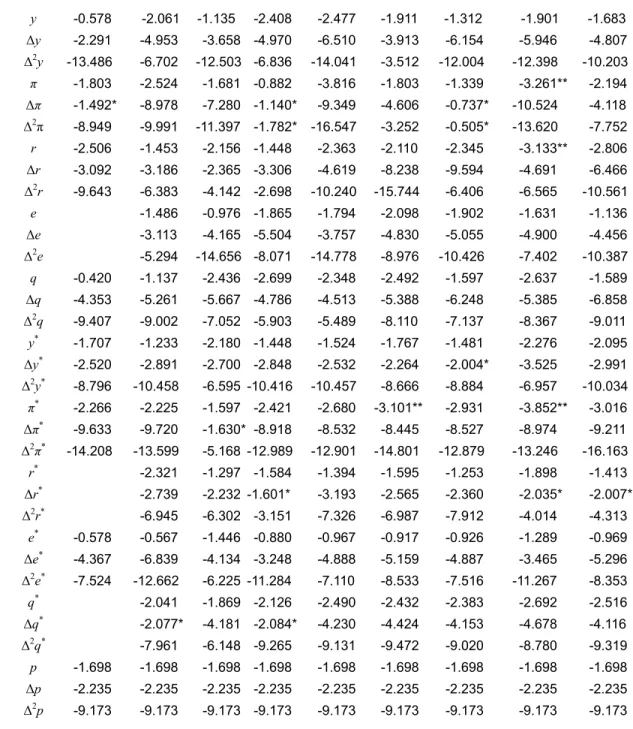
Although the GVAR methodology can be applied to stationary and/or integrated variables, the assumption that the variables included in the country-specific models are integrated of order one (or I(1))—in Pesaran et al. (2004), Dees et al. (2007), and Pesaran et al. (2009)—still plays an important role. The assumption allows us to distinguish short- and long-run relations and interpret those long-run as co-integrating. Therefore, we begin our tests by examining the integration properties of the individual series under consideration. Due to the widely accepted poor power performance of the traditional augmented Dickey-Fuller (ADF) tests, we use the ADF-GLS statistics introduced by Elliot, Rothenberg, and Stock (1996) for all series in Table 5. With only a few exceptions, the I(1) assumption cannot be rejected for most of the endogenous and exogenous variables under consideration.9

4.2. Testing Weak Exogeneity

The main assumption underlying the estimation strategy is the weak exogeneity of X_it∗

with respect to the long-run parameters of the VECMX* model defined by (3). Following Dees et al. (2007), we can check the weak exogeneity by testing the joint significance of the estimated error-correction terms defined by (4) for the country-specific foreign variables and world commodity prices. In particular, for each lth element of X_it∗_the

following regression is carried out:

_, _{, ,} _{, 1} _, _, _1, _{, 1} _, 1 1 i i r s j it l il i j l i t ik l i t k i l i t it l j k

X

∗

μ

γ

ECM

ϕ

X

υ

X

∗

ς

− − − = =

Δ

=

+

∑

+

∑

Δ

+

Δ

%

+

(9)

9_{Nevertheless, some of the variables used in the country-specific models seem to be}

I(2), for example, US inflation, and some even seem to be I(3), for example, Japanese inflation.

(17)

where j_{, 1}

, 1, 2, ,

i t i

ECM

₋

j

=

_L

r

are the estimated error-correction terms corresponding to the ri co-integrating relations found for the ith country model, si = pi (the lag order of

endogenous variables in the ith country model), and ( , , W)

it it it t X∗ X′∗ e∗ p ′

Δ% = Δ Δ Δ . Note that in the case of the US the term Δe_it∗ is implicitly included in ΔX_it∗. The test for weak exogeneity is an F-test of the joint hypothesis that

γ

i j l_{, ,} =0, j=1, 2, ,L ri in the above regression. The test results are summarized in Table 6.

As can be seen from this table, the weak exogeneity assumptions for the countries under consideration are rejected only for inflation in the US model and the short-term interest rate in the Thai model. As expected, foreign real equity prices and foreign short-term interest rates cannot be considered as weakly exogenous and have not been included in the US model, which justifies the importance of US financial markets within the global financial system.

4.3. Other Features of the Country-Specific Models

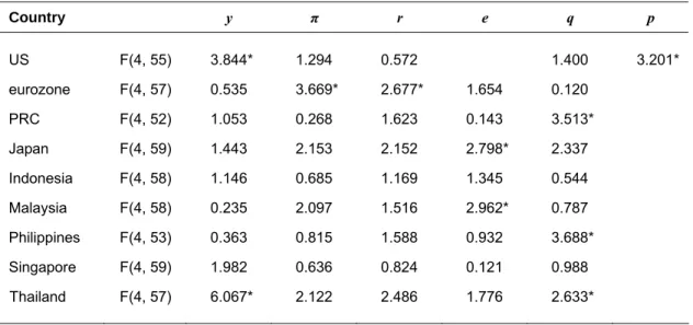
Due to data limitations and the relatively large number of endogenous and exogenous variables involved, we were forced to set the lag order of exogenous variables for all country-specific models at one. It is therefore important to check the adequacy of the country-specific models in dealing with the complex dynamic interrelationships that exist in the world economy. To this end, Table 7 provides F-statistics for Breusch-Godfrey LM tests of serial correlation of order 4 in the residuals of the error-correction regressions for all 45 endogenous variables in the GVAR model.

Considering the relative simplicity of the underlying models, it is comforting that 35 of the 45 regressions pass the residual serial correlation test at the 95% level. In particular, if we focus on ASEAN-5, only 4 out of the 20 regressions fail to pass the test at the 95% level. These test results, together with the weak exogeneity of the foreign variables, also allow consistent estimation of the contemporaneous effects of foreign-specific variables on their domestic counterparts (at least for the ones where the residual serial correlation test is not statistically significant).

4.4. Contemporaneous Effects of Foreign Variables on Domestic

Counterparts

Table 8 presents the contemporaneous effects of foreign variables on their domestic counterparts together with Newey-West heteroskedasticity and autocorrelation consistent (HAC) covariance matrix estimator. These estimates can be interpreted as impact elasticities between domestic and foreign variables. In Singapore, for example, a 1% change in foreign real GDP in a given quarter leads to an increase of 1.14% in domestic real GDP within the same quarter. Similar foreign elasticities are obtained across the different countries/regions.

Most of these elasticities are significant and have a positive sign, which are consistent with the results in Dees et al. (2007), except the foreign short-term interest rate of the

(18)

PRC and the foreign inflation of Japan. Focusing on ASEAN-5, foreign real GDP in Malaysia, Singapore, and Thailand, and foreign inflation in Malaysia, the Philippines, and Thailand have significant and positive contemporaneous effects on their domestic counterparts. In addition, the foreign equity prices in all ASEAN-5 countries have significant and positive effects on their domestic counterparts, suggesting contemporaneous financial links are likely to be very strong among ASEAN-5 economies through the equity market channel. Another interesting finding is that neither foreign real GDP nor foreign inflation has a significant effect on their domestic counterparts in the PRC and Indonesia—which may imply the two economies are not as open as the other countries/regions under consideration.

5. Forecast and Evaluation

5.1. Forecast Results

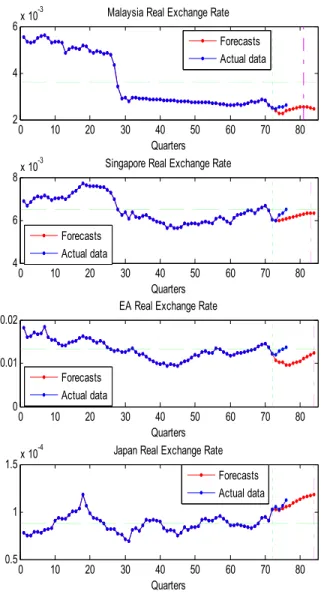
We compute the one quarter ahead forecasts for 2009Q1–2011Q4. Figure 1 presents real GDP growth forecasts for all the countries under consideration. We can see that the real GDP growth forecasts for all countries expect Thailand have a clear downward trend in 2011. Figures 2, 3, 4, and 5 present forecasts for inflation, short-term interest rates, real exchange rates, and real equity prices respectively.

It is necessary to evaluate how well these forecasts perform compared with other models. We consider two benchmark models used in the forecast evaluation. We apply the panel Diebold and Mariano (DM) test developed by Pesaran et al. (2009)—which allows us to statistically test the GVAR forecasts against our benchmark models for a given variable. Note that we have only four One quarter ahead forecasts (obtained over 2009Q1–2009Q4) for each of the variables and for each country, which is insufficient for statistical testing of forecasts for individual countries. However, by pooling forecast errors for the same variable across different countries, the panel DM test is able to take into account the panel nature of the pooled series.

5.2. Benchmark Models

We compare the forecast performance of the GVAR model with that of forecasts from country-specific VAR(2) models, with and without trend. The specifications of the two benchmark models are

1 , 1 2 , 2

Country-specific VAR(2):

Country-specific VAR(2) with trend:

it i t i t it it i t i t it X a X X X a bt X X

γ

ξ

γ

ξ

− − − − = + + + ⎧⎪ ⎨ = + + + + ⎪⎩ where i = 0, 1, 2, …, N.

VAR(2) models are chosen for two reasons: (i) they usually perform very well in forecasting; and more importantly, (ii) the only feature they don’t possess compared with the GVAR model is global interdependency. Thus, if the GVAR model outperforms these

(19)

VAR(2) models, then the global interrelationships should be considered important in forecasting. The forecast is based on the conditional expectation in the usual manner for VAR models.

5.3. Forecast Evaluation

To derive the panel DM test, we first consider the loss differential of forecasting the variable j in country i, using method A relative to method B:

( ) ( )

2 2

,

GVAR forecast,

Benchmark forecast,

A B

ijt ijt ijt

z

e

A

B

=

−

≡

for i = 1, 2, …, m; j = 1, 2, …, k; and t = 1, 2, …, n; and where m is the number of countries (m= 9), k is the number of variables, and n is the forecast sample (n = 4).

1

ˆ

1 , 1

t t t t t

e

=

y

₊

−

y

₊ ₋ is the one quarter ahead forecast error, with

y

_t₊₁ being the actual value and

y

ˆ

_t₊_{1 , 1}_{t t}₋ the corresponding forecast formed at time t.

The panel DM statistic, as developed in Pesaran et al. (2009), is defined as follows: For a given variable (say, real GDP growth), consider

₀ 1

,

:

0,

:

0, for some ,

it i it i i

z

H

i

α ε

α

=

+

=

<

suppressing the variable index j for simplicity. As shown in Pesaran et al. (2009), under the null hypothesis, and assuming that

ε

_it

~ . . .(0,1)

i i d

, then

~

(0,1)

( )

z

DM

N

V z

=

, where: 2 2

(

)

2 1 1 1 1

1

1 ,

,

( )

,

1

m n m n i i it i i it i i t j t

z

V z

z

m

=

n

=

mn

m

=

σ

n

=

⎛

⎞

⎛

⎞

=

_⎜

_⎟

_⎜

_⎟

=

−

⎝

_⎠⎝

_⎠

∑

)

∑

_.

Note that the panel DM test defined above is a one-sided test, so that the relevant 1% and 5% critical values are -2.326 and -1.645, respectively. Thus, assuming the GVAR forecast is defined as A, a positive value of the panel DM statistic presents evidence against it.

(20)

Table 9 presents the panel DM statistics for the One quarter ahead GVAR forecasts relative to the two benchmark models. We can see in the table that there is no evidence against the GVAR forecasts as the statistics for all variables are negative. In particular, the statistics for the short-term interest rate compared with both benchmarks are significantly negative at the 5% level, indicating that the GVAR forecasts are very likely to beat those from the VAR(2) models with or without trend.

6. Generalized Impulse Response Functions

To study the dynamic properties of the global model and to assess the time profile of the effects of shocks to foreign variables on ASEAN-5 economies, we investigate the implications of three different external shocks: (i) a one standard error negative shock to US real equity prices; (ii) a one standard error positive shock to US interest rates; and (iii) a one standard error positive shock to world commodity prices. Here we make use of the generalized impulse response function (GIRF), proposed in Koop et al. (1996), developed further in Pesaran and Shin (2002) for vector error-correcting models, and applied by Pesaran et al. (2004) and Dees et al. (2007) in the GVAR model. The GIRF is an alternative to the orthogonalized impulse responses (OIR) of Sims (1980). The OIR approach requires the impulse responses to be computed with respect to a set of orthogonalized shocks, while the GIRF approach considers shocks to individual errors and integrates out the effects of the other shocks using the observed distribution of all the shocks without any orthogonalization. Unlike the OIR, the GIRF is invariant to ordering variables and the countries in the GVAR model—clearly an important consideration. Even if a suitable ordering of the variables in a given country model derives from economic theory or general a priori reasoning, it is not clear how to order countries when applying the OIR to the GVAR model.10

Supplement A in Dees et al. (2007) provides a way to compute the GIRF. On the assumption that the error term

ε

_t associated with equation (7) has a multivariate normal distribution, the

k

×

1

vector of the GIRFs in the case of a one standard error shock to the jth equation corresponding to a particular shock in a particular country on Xt+n is given

by 1 , , 0,1, 2, n u j j n j u j F G l GI n l l −_Σ = = ′Σ % L (10) where l_j is a

k

×

1

selection vector with unity as its jth element,

Σ

_u is the (estimated) covariance matrix of

ε

_t estimated by

( )

0,1, , 0,1, , ˆ _i _N u ij j N

σ

= = Σ = _L L

(21)

ASEAN-5 Macroeconomic Forecasting Using a GVAR Model | 13 where 1 1

ˆ

_ij T _it _jt t

T

σ

−

ε ε

=

′

=

∑

) )

,

ε

)

_it is the residual in (3) obtained by plugging in all the coefficient estimates:

F

%

=

E FE

₁ ₁

′

, with 1 2

0

k k k

F

I

_×

⎛

⎞

= ⎜

⎟

⎝

⎠

and

E

1

=

(

I

k

0

k k×

)

. This

result also holds in non-Gaussian but linear settings, where the conditional expectations can be assumed to be linear.11

In discussing the results, we focus only on the first 3 years following the shock. Figures 6-11 present the GIRFs for shocks to US real equity prices, world commodity prices, and US short-term interest rates. The figures show that some of the GIRFs for ASEAN-5 do not settle down very quickly, suggesting that either the effects of the shocks are quite persistent or the model is a little unstable. If it were the second case, then it might be due to data limitations, or the fact that we found in the section of unit root tests, namely, some of the variables are I(2) or even I(3). As for the latter, higher differences or year-to-year changes might be able to stabilize GIRFs.

7. Conclusion

In this paper we examine and evaluate the macroeconomic forecasts for ASEAN-5 countries in the context of a global vector autoregressive (GVAR) model covering 20 countries grouped into nine country/regions. We generate 12 One quarter ahead forecasts of real GDP, inflation, short-term interest rates, real exchange rates, real equity prices, and world commodity prices over the 2009Q1–2011Q4 period—with four out-of-sample forecasts covering 2009Q1–2009Q4. The out-of-sample forecasts are compared with country-specific vector autoregressive models with and without trend. The forecast evaluation results indicate that the GVAR forecasts tend to outperform forecasts based on individual country-specific models (the VAR(2) benchmark models), especially for short-term interest rates and real equity prices, implying the importance of interdependence with global financial markets.

There are many extensions we can make in the future. One is to apply Phillips’ semi-parametric approach, the fully modified vector autoregression (FMVAR)—robust to error distributions—to estimate the country-specific VARX* models, and compare the results with the results in this paper. One extension is to include more countries in the sample as well as to extend the sample period. Another extension is to estimate different models according to pi and qi, as well as estimation windows, and use Bayesian model

averaging to integrate the uncertainties that prevail across models and across estimation windows.12_{Note that these three extensions can be made simultaneously.}

11_{See Supplement A in Dees et al. (2007).} 12_{See Pesaran et al. (2009) for details.}

(22)

Table 1: Trade Weights Based on Direction of Trade Statistics

US = United States; PRC = People’s Republic of China.

Note: Trade weights are computed as shares of exports and imports, displayed in rows by region (such that a row, but not a column, sum to 1).

Source: Direction of Trade Statistics, 2007–2009, International Monetary Fund.

Table 2: Co-Integration Rank Statistics for the US Model (3 exogenous variables)

Critical Values1

H0 H1 US

95% 90%

Maximum Eigenvalue Statistics

r = 0 _{r = 1} _72.107 _46.84 _43.92 r = 1 _{r = 2} _48.937 _40.98 _38.04 r = 2 _{r = 3} 24.807 34.65 31.89 r = 3 _{r = 4} _19.088 _27.80 _25.28 r = 4 _{r = 5} _8.9249 _20.47 _18.19 Trace Statistics r = 0 _r_≥₁ _173.87 _120.0 _114.7 r = 1 _r_≥₂ _101.76 _90.02 _85.59 r = 2 _r_≥₃ _52.82 _{63.54 59.39} r = 3 _r_≥₄ _28.013 _40.37 _37.07 r = 4 r ≥ 5 8.9249 20.47 18.19

Note: The critical values are from Table 6 (d) in Pesaran et al (2000) as the country-specific models belong to

case IV in their paper.

US eurozone PRC Japan Indonesia Malaysia Philippines Singapore Thailand

US 0.000 0.346 0.317 0.149 0.024 0.051 0.020 0.0537 0.0390 eurozone 0.429 0.000 0.330 0.119 0.021 0.031 0.009 0.0373 0.0247 PRC 0.307 0.281 0.000 0.233 0.026 0.046 0.025 0.0474 0.0352 Japan 0.271 0.168 0.338 0.000 0.051 0.047 0.024 0.0413 0.0607 Indonesia 0.123 0.125 0.152 0.228 0.000 0.085 0.016 0.2140 0.0574 Malaysia 0.178 0.137 0.161 0.160 0.053 0.000 0.021 0.2123 0.0773 Philippines 0.215 0.152 0.144 0.207 0.028 0.061 0.000 0.1308 0.0619 Singapore 0.161 0.139 0.170 0.105 0.131 0.202 0.033 0.0000 0.0607 Thailand 0.157 0.134 0.185 0.260 0.053 0.097 0.028 0.0853 0.0000

(23)

Table 3: Co-Integration Rank Statistics for Non-US Countries/East Asia (5 exogenous variables)

Critical

Values1

H0 H1 eurozone PRC Japan Indonesia Malaysia Philippines Singapore Thailand

95% 90%

Maximum Eigenvalue Statistics

r = 0 r = 1 89.797 85.204 104.2 77.736 72.905 74.647 53.8 77.919 52.63 49.59 r = 1 r = 2 52.58 54.632 85.791 53.022 53.07 50.001 44.526 58.726 46.66 43.66 r = 2 r = 3 43.286 33.154 30.35 43.84 38.918 28.4 35.158 40.488 40.12 37.28 r = 3 r = 4 27.448 24.168 28.031 34.791 27.72 23.794 28.316 38.261 33.26 30.54 r = 4 r = 5 21.106 20.296 17.813 26.484 19.397 18.548 11.074 20.394 25.70 23.11 Trace Statistics r = 0 r ≥1 234.22 217.45 266.18 235.87 212.01 195.39 172.87 235.79 141.2 135.8 r = 1 r ≥2 144.42 132.25 161.99 158.14 139.11 120.74 119.07 157.87 107.6 102.5 r = 2 r ≥3 91.84 77.618 76.195 105.11 86.035 70.742 74.547 99.143 76.82 72.33 r = 3 r ≥4 48.554 44.464 45.845 61.275 47.117 42.342 39.389 58.655 49.52 46.10 r = 4 r ≥5 21.106 20.296 17.813 26.484 19.397 18.548 11.074 20.394 25.70 23.11

PRC= People’s Republic of China.

Note: The critical values are from Table 6(d) in Pesaran et al (2000) since the country-specific models belong to case IV in

their paper.

Table 4: VARX* Order and Number of Co-Integration Relationships in the Country-Specific Models Country/Region VARX*(pi, qi) # Co-integrating relationships pi qi US 2 1 2 Eurozone 2 1 3 PRC 2 1 3 Japan 1 1 2 Indonesia 2 1 4 Malaysia 2 1 3 Philippines 2 1 2 Singapore 1 1 2 Thailand 1 1 4

(24)

Table 5: ADF-GLS Unit Root Test Statistics (based on MAIC order selection)

Domestic

Variables US eurozone PRC Japan Indonesia Malaysia Philippines Singapore Thailand

y -0.578 -2.061 -1.135 -2.408 -2.477 -1.911 -1.312 -1.901 -1.683 Δy -2.291 -4.953 -3.658 -4.970 -6.510 -3.913 -6.154 -5.946 -4.807 Δ2_y _{-13.486 -6.702 -12.503 -6.836 -14.041 -3.512 -12.004 -12.398 -10.203} π -1.803 -2.524 -1.681 -0.882 -3.816 -1.803 -1.339 -3.261** -2.194 Δπ -1.492* -8.978 -7.280 -1.140* -9.349 -4.606 -0.737* -10.524 -4.118 Δ2_π _{-8.949 -9.991 -11.397 -1.782* -16.547 -3.252 -0.505* -13.620 -7.752} r -2.506 -1.453 -2.156 -1.448 -2.363 -2.110 -2.345 -3.133** -2.806 Δr -3.092 -3.186 -2.365 -3.306 -4.619 -8.238 -9.594 -4.691 -6.466 Δ2_r _{-9.643 -6.383 -4.142 -2.698 -10.240 -15.744 -6.406} _{-6.565 -10.561} e -1.486 -0.976 -1.865 -1.794 -2.098 -1.902 -1.631 -1.136 Δe -3.113 -4.165 -5.504 -3.757 -4.830 -5.055 -4.900 -4.456 Δ2_e _{-5.294 -14.656 -8.071 -14.778 -8.976 -10.426 -7.402 -10.387} q -0.420 -1.137 -2.436 -2.699 -2.348 -2.492 -1.597 -2.637 -1.589 Δq -4.353 -5.261 -5.667 -4.786 -4.513 -5.388 -6.248 -5.385 -6.858 Δ2_q _{-9.407 -9.002 -7.052 -5.903 -5.489 -8.110 -7.137} _{-8.367 -9.011} y* _{-1.707 -1.233 -2.180 -1.448 -1.524 -1.767 -1.481} _{-2.276 -2.095} Δy* _{-2.520 -2.891 -2.700 -2.848 -2.532 -2.264 -2.004* -3.525 -2.991} Δ2_y* _{-8.796 -10.458 -6.595 -10.416 -10.457 -8.666 -8.884} _{-6.957 -10.034} π* _{-2.266 -2.225 -1.597 -2.421 -2.680 -3.101** -2.931} _{-3.852** -3.016} Δπ* _{-9.633 -9.720 -1.630* -8.918 -8.532 -8.445 -8.527} _{-8.974 -9.211} Δ2_π* _{-14.208 -13.599}_{-5.168 -12.989 -12.901 -14.801 -12.879 -13.246 -16.163} r* _{-2.321 -1.297 -1.584 -1.394 -1.595 -1.253} _{-1.898 -1.413} Δr* _{-2.739 -2.232 -1.601* -3.193 -2.565 -2.360} _{-2.035* -2.007*} Δ2_r* _{-6.945 -6.302 -3.151 -7.326 -6.987 -7.912} _{-4.014 -4.313} e* _{-0.578 -0.567 -1.446 -0.880 -0.967 -0.917 -0.926} _{-1.289 -0.969} Δe* _{-4.367 -6.839 -4.134 -3.248 -4.888 -5.159 -4.887} _{-3.465 -5.296} Δ2_e* _{-7.524 -12.662 -6.225 -11.284 -7.110 -8.533 -7.516} _{-11.267 -8.353} q* _{-2.041 -1.869 -2.126 -2.490 -2.432 -2.383} _{-2.692 -2.516} Δq* _{-2.077* -4.181 -2.084* -4.230 -4.424 -4.153} _{-4.678 -4.116} Δ2_q* _{-7.961 -6.148 -9.265 -9.131 -9.472 -9.020} _{-8.780 -9.319} p -1.698 -1.698 -1.698 -1.698 -1.698 -1.698 -1.698 -1.698 -1.698 Δp -2.235 -2.235 -2.235 -2.235 -2.235 -2.235 -2.235 -2.235 -2.235 Δ2_p _{-9.173 -9.173 -9.173 -9.173 -9.173 -9.173 -9.173} _{-9.173 -9.173}

Note: * denotes fail to reject the null hypothesis of unit root at 5% level. ** denotes reject the null hypothesis of unit root at 5% level.

(25)

Table 6: F-statistics for Testing the Weak Exogeneity of the Country-Specific Foreign Variables and Commodity Prices

Foreign variables Country y* _π* _r* _e* _q* _P US F(2, 53) 0.72 3.86* 0.93 eurozone F(4, 54) 1.24 0.39 1.08 0.67 0.52 PRC F(3, 49) 0.56 1.90 0.87 1.01 0.95 Japan F(3, 55) 1.93 1.19 0.22 0.68 0.10 Indonesia F(3, 55) 0.82 0.23 1.15 0.49 0.14 Malaysia F(3, 55) 1.53 0.62 1.16 2.65 1.76 Philippines F(2, 50) 0.53 0.80 2.41 0.16 0.27 Singapore F(2, 56) 0.05 0.33 0.15 0.96 1.39 Thailand F(4, 54) 1.12 2.22 3.85* 0.87 2.03

US = United States; PRC = People’s Republic of China. Note: * denotes statistical significance at the 5% level.

Table 7: F-statistics for Tests of Residual Serial Correlation for Country-Specific VARX* Models

Country y π r e q p US F(4, 55) 3.844* 1.294 0.572 1.400 3.201* eurozone F(4, 57) 0.535 3.669* 2.677* 1.654 0.120 PRC F(4, 52) 1.053 0.268 1.623 0.143 3.513* Japan F(4, 59) 1.443 2.153 2.152 2.798* 2.337 Indonesia F(4, 58) 1.146 0.685 1.169 1.345 0.544 Malaysia F(4, 58) 0.235 2.097 1.516 2.962* 0.787 Philippines F(4, 53) 0.363 0.815 1.588 0.932 3.688* Singapore F(4, 59) 1.982 0.636 0.824 0.121 0.988 Thailand F(4, 57) 6.067* 2.122 2.486 1.776 2.633*

US = United States; PRC = People’s Republic of China. Note: * denotes statistical significance at the 5% level.

(26)

Table 8: Contemporaneous Effects of Foreign Variables on their Domestic Counterparts

Domestic variables Country y π r q US 0.488*** _(0.15) 0.224*** _(0.081) eurozone 0.195 _(0.148) 0.291*** _(.0432) 0.451*** _(0.157) 0.447*** _(.1661612) PRC -0.094 _(0.177) 0.139 _(0.335) -0.156** _(0.077) -0.136 _(0.286) Japan 0.399* _(0.223) -0.144** _(0.059) -0.036 _(0.054) 0.066 _(0.179) Indonesia -0.164 _(0.541) 1.143 _(0.770) 5.256** _(2.574) 1.327** _(0.162) Malaysia 1.313*** _(0.211) 0.938*** _(0.257) 0.206 _(0.151) 0.716*** _(0.186) Philippines 0.112 _(0.250) 1.376*** _(0.295) 2.761*** _(0.923) 1.243*** _(0.138) Singapore 1.137*** _(0.307) 0.038 _(0.093) 0.127 _(0.110) 0.925*** _(0.119) Thailand 1.015** _(0.459) 0.310** _(0.146) 3.766*** _(0.502) 1.186*** _(0.258)

Note: Newey-West HAC standard errors are given in parentheses. * denotes statistical significance at the 10% level, ** denotes statistical significance at the 5% level, and *** denotes statistical significance at the 1% level.

Table 9: Panel DM Statistics for GVAR Forecasts Relative to the Benchmark Model, 2009Q1–2009Q4

Benchmark Model

Real GDP

Growth Rate Inflation

Short-Term Interest Rate Real Exchange Rate Real Equity Price Country-specific VAR(2) -0.291 -0.210 -2.093* -0.480 -0.961 Country-specific

VAR(2) with trend -0.253 -0.815 -2.199* -0.599 -1.113

Notes: * denotes statistical significance at the 5% level. A positive value of the panel DM statistic represents evidence against the GVAR forecasts.

(27)

ASEAN-5 Macroeconomic Forecasting Using a GVAR Model | 19 0 20 40 60 80 -20 -10 0 10 20 Quarters

Indonesia Real GDP Growth Rate (%)

0 20 40 60 80 -10 -5 0 5 10 Quarters

Malaysia Real GDP Growth Rate (%)

0 20 40 60 80

-5 0 5

Quarters

Philippines Real GDP Growth Rate (%)

0 20 40 60 80 -10 -5 0 5 10 Quarters

Singapore Real GDP Growth Rate (%)

0 20 40 60 80 -10 -5 0 5 10 Quarters

Thailand Real GDP Growth Rate (%)

0 20 40 60 80 -2 -1 0 1 2 Quarters

US Real GDP Growth Rate (%)

0 20 40 60 80

-5 0 5

Quarters

EA Real GDP Growth Rate (%)

0 20 40 60 80 0 2 4 6 8 10 Quarters

PRC Real GDP Growth Rate (%)

0 20 40 60 80

-5 0 5

Quarters

Japan Real GDP Growth Rate (%)

Forecasts Actual data Forecasts Actual data Forecasts Actual data Forecasts Actual data Forecasts Actual data Forecasts Actual data Forecasts Actual data Forecasts Actual data Forecasts Actual data

Figure 1: One Quarter Ahead Forecasts for Real GDP Growth

(28)

Figure 2: One Quarter Ahead Forecasts for Inflation

EA= Euro Area, PRC= People’s Republic of China.

0 20 40 60 80 -50 0 50 Quarters Indonesia Inflation (%) 0 20 40 60 80 -5 0 5 Quarters Malaysia Inflation (%) 0 20 40 60 80 -10 -5 0 5 10 Quarters Philippines Inflation (%) 0 20 40 60 80 -5 0 5 Quarters Singapore Inflation (%) 0 20 40 60 80 -5 0 5 Quarters Thailand Inflation (%) 0 20 40 60 80 -5 0 5 Quarters US Inflation (%) 0 20 40 60 80 -2 -1 0 1 2 Quarters EA Inflation (%) 0 20 40 60 80 -10 -5 0 5 10 Quarters PRC Inflation (%) 0 20 40 60 80 -2 -1 0 1 2 Quarters Japan Inflation (%) Forecasts Actual data Forecasts Actual data Forecasts Actual data Forecasts Actual data Forecasts Actual data Forecasts Actual data Forecasts Actual data Forecasts Actual data Forecasts Actual data

(29)

Figure 3: One Quarter Ahead Forecasts for Short-Term Interest Rate

EA= Euro Area, PRC= People’s Republic of China.

0 20 40 60 80 0 20 40 60 80 100 Quarters

Indonesia Short-Term Interest Rate (%)

0 20 40 60 80 0 2 4 6 8 10 Quarters

Malaysia Short-Term Interest Rate (%)

0 20 40 60 80

-50 0 50

Quarters

Philippines Short-Term Interest Rate (%)

0 20 40 60 80 -10 -5 0 5 10 Quarters

Singapore Short-Term Interest Rate (%)

0 20 40 60 80 0 10 20 30 40 Quarters

Thailand Short-Term Interest Rate (%)

0 20 40 60 80 -10 -5 0 5 10 Quarters

US Short-Term Interest Rate (%)

0 20 40 60 80 -20 -10 0 10 20 Quarters

EA Short-Term Interest Rate (%)

0 20 40 60 80 0 2 4 6 8 10 Quarters

PRC Short-Term Interest Rate (%)

0 20 40 60 80 -10 -5 0 5 10 Quarters

Japan Short-Term Interest Rate (%)

Forecasts Actual data Forecasts Actual data Forecasts Actual data Forecasts Actual data Forecasts Actual data Forecasts Actual data Forecasts Actual data Forecasts Actual data Forecasts Actual data

ASEAN-5 Macroeconomic Forecasting Using a GVAR Model