Multi-Telescope Radio Observations for Low Frequency Gravitational Wave Astrophysics

(1)

Graduate Theses, Dissertations, and Problem Reports 2018

Multi-Telescope Radio Observations for Low Frequency

Gravitational Wave Astrophysics

Megan L. Jones

West Virginia University, mljones1@mix.wvu.edu

Follow this and additional works at: https://researchrepository.wvu.edu/etd

Part of the Cosmology, Relativity, and Gravity Commons, and the Stars, Interstellar Medium and the Galaxy Commons

Recommended Citation Recommended Citation

Jones, Megan L., "Multi-Telescope Radio Observations for Low Frequency Gravitational Wave Astrophysics" (2018). Graduate Theses, Dissertations, and Problem Reports. 3723.

https://researchrepository.wvu.edu/etd/3723

This Dissertation is protected by copyright and/or related rights. It has been brought to you by the The Research Repository @ WVU with permission from the rights-holder(s). You are free to use this Dissertation in any way that is permitted by the copyright and related rights legislation that applies to your use. For other uses you must obtain permission from the rights-holder(s) directly, unless additional rights are indicated by a Creative Commons license in the record and/ or on the work itself. This Dissertation has been accepted for inclusion in WVU Graduate Theses, Dissertations, and Problem Reports collection by an authorized administrator of The Research Repository @ WVU.

(2)

Multi-Telescope Radio Observations for

Low Frequency Gravitational Wave

Astrophysics

Megan L. Jones

Dissertation Submitted to

The Eberly College of Arts and Sciences at West Virginia University in partial fulfillment of the requirements

for the degree of

Doctor of Philosophy in

Physics

Maura McLaughlin, Ph.D., Chair James M. Cordes, Ph.D. Sarah Burke-Spolaor, Ph.D. Kathryn Williamson, Ph.D.

Morgantown, West Virginia, USA 2018

(3)

Abstract

Multi-Telescope Radio Observations for Low Frequency Gravitational Wave Astrophysics

Megan L. Jones

The North American Nanohertz Observatory for Gravitational Waves (NANOGrav) has the principal goal of detecting gravitational waves (GWs) in the nanohertz part of the spectrum using pulsar timing. This thesis presents results from radio campaigns at frequencies from 322 MHz to 10 GHz aimed at both multi-messenger constraints on GW sources and improving the timing sensitivity. The primary expected source of GWs at the nanohertz frequen-cies to which pulsar timing is sensitive are supermassive black hole (SMBH) binaries. We investigate a purported SMBH displaced from the galactic pho-tocenter in NGC 3115. We explore the possibilities that the source is a SMBH binary or a post-merger recoiling SMBH. We place constraints on a possible SMBH companion using observations taken with the NRAO Very Large Ar-ray. If a companion SMBH can be confirmed, this system could be a future GW source detectable with pulsar timing.

In order to detect such sources, our pulsar timing array must be as sensitive as possible, requiring the mitigation of all other astrophysical delays, including those from the interstellar medium (ISM). Using NANOGrav wideband multi-frequency observations obtained with the Green Bank Telescope and Arecibo Observatory, we characterize frequency-dependent dispersion. This effect is quantified by the dispersion measure (DM). We analyze trends in the DM time series, propose sources of these trends, and identify timescales over which the DM varies beyond measurement errors and therefore can no longer be modeled as constant in timing. Analyzing DM variations aids in characterizing properties of the ISM and informs our timing observation strategy.

Multi-telescope observations around the globe and at complementary fre-quencies can be used to more sensitively constrain DMs. We compare DMs measured with dual-frequency observations obtained using the Giant Metre-wave Radio Telescope (GMRT) to those calculated in the NANOGrav 11-year data release to assess the possible precision of frequency-dependent noise mea-surements with the GMRT. We discuss the possibility of incorporating the GMRT into international pulsar timing efforts and anticipated challenges in future data combination.

(4)

Acknowledgements

First, I would like to thank Maura McLaughlin for all of her guidance over the past five years, and for telling me time and time again that everything was going to be alright. I cannot imagine a better or more supportive advisor. I would also like to thank my committee members for their investment in my doctoral success: Jim Cordes for his seemingly infinite wisdom and willingness to share it, Sarah Burke-Spolaor for being so cool and sharing her data wizardry with me, and Kathryn Williamson for helping me build my confidence in front of a crowd and in life.

I would like to thank my undergraduate advisor Eric Wilcots for giving me my start in astronomy research as a plucky teenager, and for helping me find my way both in undergrad and after. Thank you for always giving me good advice, and for guiding me when I could not see the forest through the trees.

Thank you to my numerous colleagues in the NANOGrav collaboration. Among you are my friends, mentors, and role models; it takes a village, and you all are my village. Thank you also to my friends and fellow graduate students at WVU. Grad school would not have been surmountable without our camaraderie and beer ther-apy. Particular thanks to my best friend Tom, who is always up for long chats, late night proofreading, and who always makes me laugh. A huge thank you to Michael Lam for being my professional and emotional co-pilot, and for keeping me fueled with the best ramen ever while writing this thesis.

Above all, I would like to thank my parents, Gail and Richard, for their unceas-ing, unwaverunceas-ing, and unconditional support. They taught me to see no limitations and that the stars were (literally) the limit. I would not be the person I am today without their care and guidance.

(5)

4 Evaluating Low Frequency Observations at the GMRT 89 4.1 Abstract . . . 89 4.2 Introduction . . . 90 4.3 Data . . . 99 4.4 Comparison of DM measurements . . . 101 4.4.1 PSR J0030+0451 . . . 105 4.4.2 PSR J1640+2224 . . . 105 4.4.3 PSR J1713+0747 . . . 106 4.4.4 PSR J2145–0750 . . . 107 4.5 Conclusions . . . 108 5 Conclusion 111 5.1 Importance of DM characterization and understanding the ISM . . . 111

5.2 Investigating a potential SMBH binary candidate . . . 112

5.2.1 Data combination and PTA data standards . . . 113

(7)

List of Tables

2.1 Properties of NANOGrav MSPs in the 9-Year Data Release. . . 34

2.2 Fitted Trends in the DM Time Series for MSPs in the 9-Year Release 35 2.3 Diffractive timescales for 18 MSPs . . . 56

2.4 Positions and Corrected Velocities For Three MSPs . . . 58

2.5 Significance of DM peaks for MSPs within 10◦ of the ecliptic . . . 62

3.1 Astrometric Position Comparison of Sources at Other Frequencies . . 80

4.1 NANOGrav Observing Frequencies . . . 98

4.2 GMRT observation lengths . . . 100

4.3 DM estimates using low frequency GMRT data . . . 102

(8)

List of Figures

1.1 Coverage of experiments across the GW spectrum. . . 2

1.2 Polarization of a GW. . . 6

1.3 Small galaxies merge to form larger galaxies. . . 8

1.4 The P- ˙P diagram. . . 12

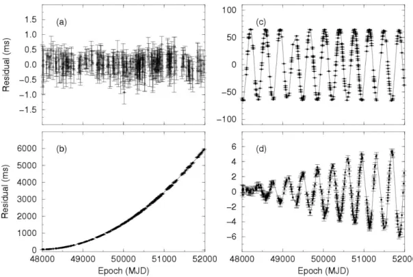
1.5 Effects on timing residuals due to errors in the timing model. . . 13

1.6 Jitter in simulated pulse profiles. . . 15

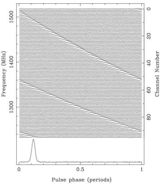
1.7 Pulse profiles for PSR J1713+0747. . . 16

1.8 The Hellings-Downs curve. . . 18

1.9 Frequency-dependent dispersion. . . 20

1.10 DM variations. . . 22

1.11 Pulse scattering. . . 23

2.1 DM time series for eight pulsars. . . 38

2.2 DM time series for eight more pulsars. . . 39

2.5 DM time series for five more pulsars. . . 42

2.6 MSP positions with respect to the ecliptic. . . 44

2.7 DM variations with respect to the solar position angle. . . 45

2.8 MSP trajectories plotted with DM color mapping at each epoch. . . . 47

2.12 Structure functions for the DM variations. . . 51

2.13 Structure functions for the DM variations. . . 52

2.14 Lomb-Scargle periodogram for PSR J0645+5158. . . 58

3.1 Contours of the 10-GHz emission from NGC 3115. . . 77

3.2 StokesIemission centered on a background source with an X-ray and ugi counterpart. . . 79

3.3 Flux density with different frequencies. . . 81

3.4 The relative positions of the data listed in Table 3.1, with our 10 GHz radio image shown in greyscale. . . 84

4.1 DM affecting the pulse arrival time for different frequencies. . . 95

(9)

Chapter 1 Introduction

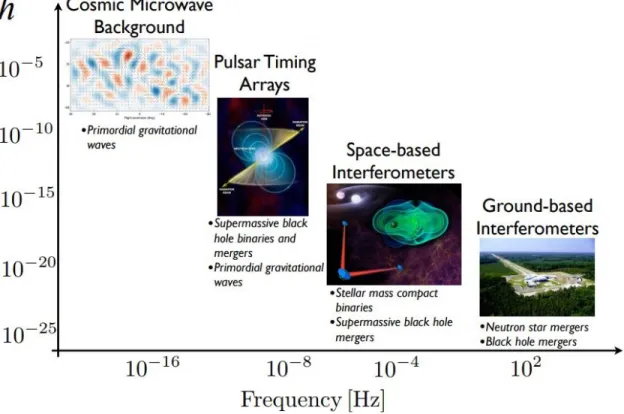
With the detection of gravitational waves (GWs) by the Laser Interferometer Gravitational-Wave Observatory (LIGO), we have entered a new era in GW as-tronomy. GW astronomy is necessary for studying phenomena only visible through gravitational dynamics and provides a multi-messenger view of processes in the Uni-verse, like supermassive black hole (SMBH) binary mergers. GW frequencies are determined by their sources; for example, SMBH binaries in ∼year orbits emit low-frequency GWs, while binaries nearing mergers emit much higher low-frequency GWs. A variety of experiments and observatories are needed to provide coverage across the GW spectrum, seen in Figure 1.1. GW detections in lower frequency regions would be complementary to those already achieved by LIGO and would offer characteriza-tion of the GW universe through the observacharacteriza-tion of a diverse populacharacteriza-tion of sources. A pulsar timing array (PTA), which is made up of an accurately timed network of precise stellar rotators called pulsars, is a low-frequency GW experiment which can be used to look for a correlated signal across multiple pulsars in the network. PTAs are formed by observing pulsars using radio telescopes here on Earth, creating a Galactic scale interferometer.

In this chapter, we will give a brief description of GWs, their detection, sources, as well as pulsar timing and the effects of the interstellar medium.

(10)

Figure 1.1 Coverage of experiments across the GW spectrum and the detectable sources in each regime. Image credit: NANOGrav.

(11)

1.1 Gravitational waves

The need for an improved gravitational theory over the Newtonian description can be seen from looking at how classical mechanics deals with gravitational force

F = Gm1m2

r2 (1.1)

where G is the gravitational constant, m1 and m2 are two masses, and r is the

distance between them. Nothing travels faster than light and information is no exception; as can be seen in Eq. 1.1, Newtonian gravity does not incorporate an explicit time dependence and therefore does not account for the time it takes for information to travel. What if the Sun’s mass was increasing over time? Equation 1.1 would go from F ∝ m toF(t) ∝ m(t), which suggests that the planets would feel this change in gravitational force at the same timet(i.e. instantaneously). This would require a speed faster than light and would violate the laws of physics.

The existence of GWs was posited by Einstein in his general theory of relativity (henceforth GR; Einstein, 1915). Contrary to Newton’s description of gravity as a force between two objects, Einstein described the influence of gravity as curvature of 4-dimensional spacetime (three spatial dimensions, and one in time); as masses move, the curvature of spacetime changes. GWs are perturbations in spacetime that propagate outward from their source at the speed of light, carrying away energy from the source system along with them.

(12)

of spacetime by contracting or elongating space. If two masses are separated by a distance L, the fractional positional perturbation they experience due to a passing GW can be described as

h= δL

L , (1.2)

where δL is the change in L due to the warping of spacetime. This fractional change h is referred to as the GW strain. GW experiments must be able to very accurately measure Lin order to detect the immensely smallδL produced by GWs. The detection of δL and the precision of that measurement are determined by the noise both intrinsic and extrinsic to the detector. It is therefore paramount for GW experiments to characterize sources of noise that may be present in the data.

1.1.1 Gravitational multipoles

While any object with mass will have a gravitational field (and will therefore warp spacetime), only certain kinds of systems will emit GWs. In order to determine which systems will be GW emitters, we must be able to characterize gravitational systems, how their mass is distributed, and how they move. It is useful to make a comparison to electromagnetism in order to describe the different properties of massive systems.

The gravitational monopole (the zeroth order term in the gravitational mul-tipole expansion) describes the total mass in a system and does not determine the emission of gravitational waves. A gravitational dipole describes how the mass is distributed. Similar to the electric dipole, the gravitational dipole can be described

(13)

as

d=X

i

mixi . (1.3)

where xi is the position vector between the two ends of the dipole. When taking the first derivative of this moment, we get the momentum

p= ˙d=X i

mix˙i , (1.4)

GWs carry energy away from the system and momentum must be conserved, there-fore gravitational dipoles also do not emit gravitational waves.

The gravitational quadrupole moment describes how masses move; it can be calculated as

q=X

i,j

(mi+mj)xixj (1.5)

For instance, a perfect non-rotating sphere moving through space has a constant quadrupole moment because from the object’s reference frame, it is at rest. In the case of a binary neutron star system however, regardless of which reference frame is used at least one of the stars is always going to be moving, giving the system a quadrupole moment that changes in time. Therefore the gravitational quadrupole is the first possible nonzero response and is the lowest order contributor to gravitational radiation.

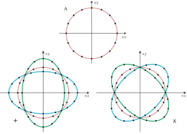
The quadrupolar nature of GWs also determines the shape of the perturbation. A GW affects spacetime by contracting or lengthening space; the directions along which space is affected in either direction depend on the polarization of the GW.

(14)

Figure 1.2 A GW affects spacetime by contracting or lengthening space; the direc-tions along which space is affected in either direction depends on the polarization of the GW. Plot A on top shows a ring of test particles unaffected by a GW. The two plots on the bottom show how the ring of test particles will behave if a GW goes through the paper. The ring of test particles initially are perturbed into stretching along the y-axis and contracting along the x-axis (shown in green), then lengthens and contracts in the other directions a half cycle later (shown in blue). Image from Wheeler (2013).

An example of GW polarizations can be seen in Figure 1.2.

1.1.2 Sources of gravitational waves

With a decade length data span and weekly to monthly observations, PTAs are sensitive to GW frequencies in the nanohertz to microhertz part of the spectrum. This portion of the GW spectrum includes continuous waves due to supermassive black hole (SMBH) binaries, the stochastic GW background made from many GW

(15)

sources in the Universe, cosmic strings, and maybe even early Universe inflation (shown in Figure 1.1). Unlike electromagnetic radiation, GWs propagate through the Universe virtually unimpeded by matter, rippling the space around them as they pass.

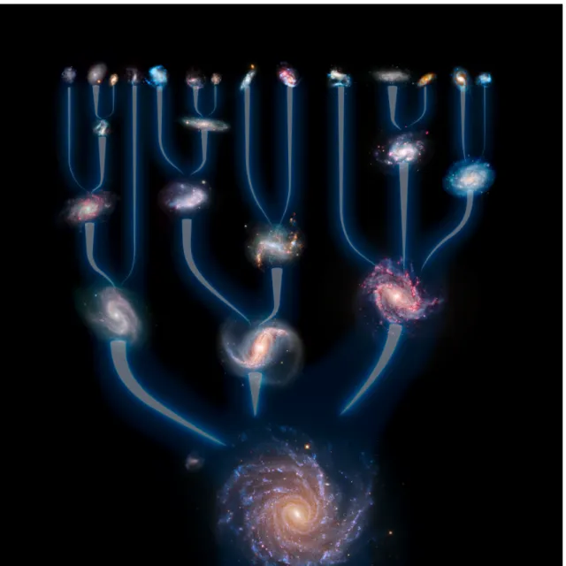
It is widely thought that most galaxies (if not all) host a SMBH at their cores; even our own Milky Way is host to a SMBH. There are several theories on the formation of SMBHs; they are even seen in the somewhat early universe (Volonteri, 2010). Galaxies grow when smaller galaxies merge and form larger galaxies; galaxy mergers also trigger large amounts of star formation. Once black holes are formed through the death of high mass stars, they grow via accretion of matter. As a black hole grows and interacts with more matter in the galaxy, it will move towards the center of the gravitational potential well (i.e. the galactic center). SMBH binaries form following major galaxy mergers. When two galaxies merge, the central SMBHs are brought together into a binary orbit through dynamical friction; as more material is consumed or ejected from the environment around this system, the binary becomes tighter and tighter.

It is at this distance that now, due to the lack of available matter left to interact with, the merging pair can stall. This is known as the final parsec problem. At first glance, the emission of GWs may appear to be a solution to this problem; GW emission results in energy being carried out of the binary system, and with this energy loss, the potential energy of the system decreases, causing the binary orbit to decay and the orbital distance to decrease. However, GW emission does not

(16)

Figure 1.3 Many smaller galaxies merge to form larger, more organized galaxies. This process continues, forming larger, more massive galaxies. Through merger dynamics, the central black holes in these galaxies grow as they absorb newly nearby material as well as other black holes. Image credit: ESO/L. Calada.

(17)

large amount of uncertainty regarding the SMBH merger rate due to the last parsec problem.

The expected strain from a SMBH binary in a circular orbit is

h'10−17M₈5/3f_yr2/−31D

−1

Gly q

(1 +q)2 , (1.6)

where M is the mass of the binary in units of 108 _M

, D is the distance to the binary, f is the frequency of the gravitational waves, and q is the mass ratio of the binary. As can be seen from Eq. 1.6, given a detectable threshold value for h, then the detection of lower frequency GWs requires higher mass black holes and/or binaries that are closer to the Earth. The detection of GWs produced by SMBH mergers will inform on the percentage of galaxy mergers that eventually produce SMBH mergers, as well as provide conclusive evidence that the final parsec problem can indeed be solved.

The time to merger for a SMBH binary is

τ = 106M₈−5/3f_yr−8−/13

(1 +q)2

q yr . (1.7)

The stochastic background spectrum is expected to follow an f−2/3 _{power law in the}

case of GW-only driven mergers. SMBH binaries with lower frequencies take more time to merge than those at higher frequencies, therefore low-frequency SMBH bina-ries have longer lifetimes. Because of this, the gravitational stochastic background is dominated by SMBH binaries with low orbital frequencies.

(18)

1.2 Pulsars

The first pulsar was discovered by graduate student Jocelyn Bell Burnell in 1967 (Hewish et al., 1968). Formed as leftover stellar cores following supernovae, pulsars are highly magnetized, rapidly rotating neutron stars. Charged particles are accelerated along the magnetic field lines of the neutron star; these particles create a beam of electromagnetic radiation as the pulsar spins. As the beam sweeps through space, scientists can detect the beam as a pulse of radiation (hence the name pulsar). The Nobel Prize was later awarded in 1974 (but not to Bell Burnell) for the discovery of pulsars.

Pulsar studies have made their way to the forefront of some of the most ground-breaking astrophysical science. The first exoplanets were discovered orbiting a pul-sar, with the Wolszczan & Frail (1992) discovery of a multi-planet system around the millisecond pulsar PSR 1257+12. The first binary pulsar PSR B1913+16 dis-covered by Hulse & Taylor (1975) earned them a Nobel Prize in 1993. It was found that over time, this binary is losing angular momentum and the orbital separation is shrinking (reviewed in Weisberg et al., 2010). This loss is consistent with predictions from general relativity (GR), providing indirect evidence of GW emission.

1.2.1 Millisecond pulsars

Pulsars spin with periods ranging from a few tens of seconds to∼1 millisecond. The first millisecond pulsar (MSP) B1937+21 was detected by Backer et al. (1982) and was determined to have a period of 1.558 ms. MSPs are defined as having

(19)

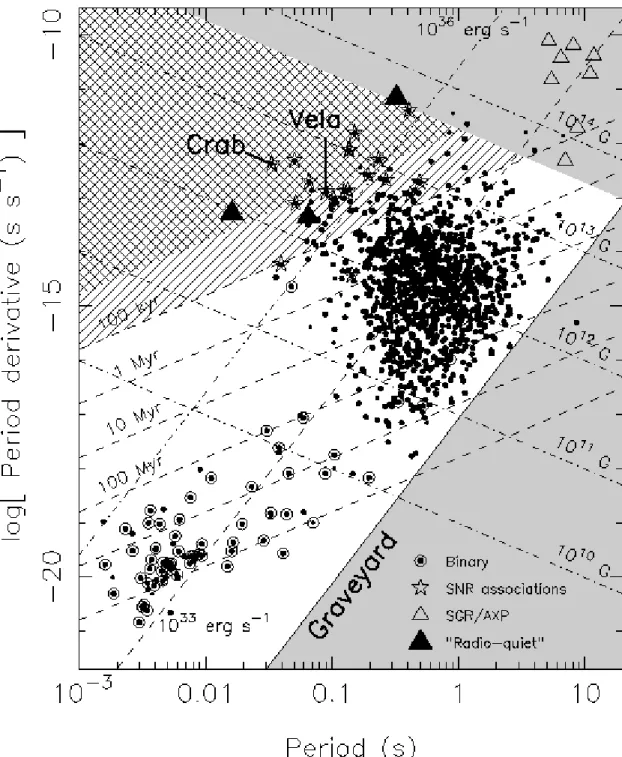
rotational periods less than ∼30 ms; these short periods are a result of the pulsars having been “recycled” or spun up after accreting material from a binary companion. As a result of this recycling, MSPs have lower magnetic fields and are more precise rotators than their slower canonical counterparts due to their lower spin-down rates, making them excellent tools for precision timing. Properties of different types of pulsars can be seen in the P −P˙ diagram in Figure 1.4. According to the ATNF Pulsar Catalogue (PSRCAT1), ∼2600 pulsars have been found to date, of which ∼350 are MSPs (Manchester et al., 2005).

1.2.2 Pulsar timing

As mentioned earlier, a GW causes a change in the length of the detector (in this case, the light travel time of the pulse). This difference in light travel time causes a change in the time of arrival (TOA) of the pulse, as a different distance means a different light travel time. GWs of the amplitude expected from SMBH binaries likely cause the TOA to vary by a few tens of nanoseconds. As a result, high precision timing is necessary in order to detect this incredibly small change in light travel time.

Due to the stability of MSP rotation periods, pulse TOAs can be predicted through pulsar timing and the determination of a timing model. A basic timing model consists of a Taylor expansion of the rotation phase φ around some initial

(20)

Figure 1.4 The P- ˙P diagram. Lines indicate constant characteristic ages, magnetic fields, and spin-down luminosity. The grey region shows forbidden regions for the pulsar population. Most of the MSPs plotted above are in binary orbits; the short periods of these pulsars are a result of them having been spun up after accreting material from their binary companion. The MSP population has smaller period derivatives compared to their spin period, and therefore make more stable rotators than canonical pulsars. Plot taken from Handbook of Pulsar Astronomy (Lorimer & Kramer, 2012).

(21)

Figure 1.5 Effects on timing residuals for PSR B1133+16 due to errors in the timing model. Plots show (a) a good timing fit, where residuals are not structured and are randomly distributed around zero, (b) an incorrect pulse spin down in the timing model, causing pulses to arrive later and later over time, (c) an error in position which causes the Earth’s motion around the Sun to be apparent in the residuals, (d) and an error in proper motion, causes an error in position that grows over time. All parameters but be fit as accurately as possible to achieve high precision in timing. Image taken from Handbook of Pulsar Astronomy (Lorimer & Kramer, 2012).

(22)

value of φo at a time to φ(t) = φo+f(t−to) + 1 2 ˙ f(t−to)2+ . . . (1.8)

where f is the pulse frequency. There are corrections for known effects that must be made before φ(t) can be predicted, making a more complex timing model. For example, effects from other planets in our Solar System, observatory clock correc-tions, and the difference in light travel time for different points in Earth’s orbit all need to be accounted for in timing. Timing models also includes a variety of spin, astrometric, and binary (where applicable) parameters that can be fit for in order to minimize the difference between our model predicted TOAs and measured TOAs. This difference in arrival time is called the residual. These parameters characterize properties both intrinsic to the pulsar as well as extrinsic, like effects on the pulse arrival time due to the ISM. Timing is done using the TEMPO2 _{software package,}

which applies a least-squares timing model fit. Errors on parameters are determined from the timing parameter covariance matrix after the least-squares fit.

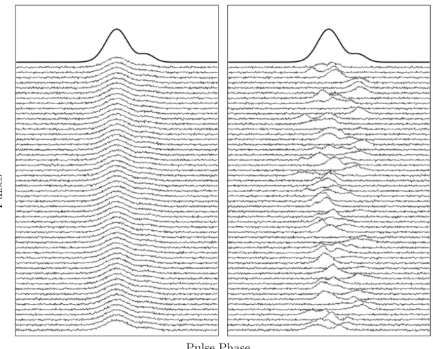
Radio emission detected from pulsars is very weak; single pulses from MSPs are often too faint to detect over the noise. In addition, the pulse shape varies between pulses. As a result, pulses need to be summed in order to construct a stable average pulse profile to be used in the timing. Jitter, intrinsic variations in the pulse shape, causes the underlying pulse to vary from the summed template and introduces noise; an example of these pulse variations can be seen in Figure 1.2.2.

(23)

Pulses

Pulse Phase

Figure 1.6 Simulated pulse data showing variations in pulse profile that cause jitter, with the summed profile appearing at the top. The simulated data on the left shows pulses that are fairly identical over time, while the pulses on the right show shape variations between pulses (i.e. jitter). Both sets of pulses results in the same averaged pulse profile.

(24)

Time (ms)

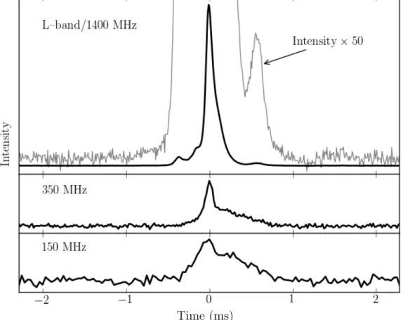
Figure 1.7 Pulse profile shapes for PSR J1713+0747 at different frequencies. The exponential tail visible at 150 and 350 MHz is caused by scattering. Plot from Dolch et al. (2014).

(25)

1.2.3 Pulsar timing array

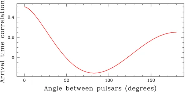
In a PTA, the Earth and a pulsar each make up an end of our GW detector; the effects of a GW on each can be described by the “Earth term” and “pulsar term” respectively. While estimates of the pulsar distance may be known, they are not precise enough to enable detection of the change in distance due a GW perturbation. As a result, the pulsar term will not be correlated between pulsars. The Earth term will show a correlation between MSPs that is related to the angular separation between pulsars. This correlation function was calculated by Hellings & Downs (1983) αij = (1−cosγij) 2 ln 1−cosγij 2 − 1 6 (1−cosγij) 2 + 1 3 , (1.9)

where γij is the angle between two pulsars (i and j) in the network. Due to the quadrupolar nature of GWs, pulsars in the same or opposite directions will show a correlated signal, while the residuals for pulsars at 90◦ angles from each other will be anti-correlated. The correlation function is illustrated by the Hellings-Downs curve, seen in Figure 1.8.

There are currently three global PTA efforts: the North American Nanohertz Observatory for Gravitational waves (NANOGrav; Arzoumanian et al., 2015), the European Pulsar Timing Array (EPTA; Desvignes et al., 2016), and the Parkes Pulsar Timing Array (PPTA; Manchester et al., 2013). These three experiments make up the International Pulsar Timing Array (IPTA; Manchester & IPTA, 2013). Other telescopes like MeerKAT and the Giant Metre-Wave Telescope (GMRT) are

(26)

Figure 1.8 The Hellings-Downs curve based on Equation 1.9. Image credit: NANOGrav.

also being used for pulsar timing, and may also be associated with future PTAs incorporated in the IPTA as well. This will be discussed more in Chapter 4.

Timing multiple pulsars forms a network of high precision Galactic clocks; this network is the PTA. The average signal-to-noise of a PTA in the intermediate GW signal limit is S/N ∝NMSPT1/2 c σ2 RM S 3/26 , (1.10)

whereNMSP is the number of MSPs in the data set,T is the length of the data span,

σ is the average rms and cis the average cadence of observations. Sensitivity of a PTA improves as more MSPs are added to the network; it is therefore essential to add as many well-timed MSPs as possible. A perturbation due to a passing GW at the Earth would create a correlated signal across the multi-pulsar network.

(27)

of observation time. Using current estimates of merger rates, the probability of a GW detection by PTAs in the next 6 years is ∼80%. PTAs will expand the range of GW astrophysics by offering constraints of the galaxy merger process, including eccentricity and stellar densities. The most recent NANOGrav limit on the GW stochastic background ish= 1.45×10−15_{at a frequency of f = 1 yr}−1 _(Arzoumanian

et al., 2018a).

1.3 The interstellar medium

Radio waves propagating through the interstellar medium (ISM) interact with this plasma in space, causing a variety of effects. The ISM is predominantly made up of hydrogen and helium that was created during the Big Bang. There is roughly one free electron for every 10 neutral hydrogen atoms (He et al., 2013).

1.3.1 Dispersion

Free electrons cause frequency-dependent dispersion of the pulse, which can be quantified by the dispersion measure (DM). The DM is the integrated column density of free electrons along the line of sight (LOS) to a pulsar

DM =

Z d

0

ne(l)dl , (1.11)

where ne is the free electron density along a LOS l and d is the pulsar distance. By assuming a model for the Galactic electron density (Cordes & Lazio, 2002, i.e.

(28)

Figure 1.9 Frequency-dependent dispersion due to free electrons in the ISM. Plot taken from Handbook of Pulsar Astronomy (Lorimer & Kramer, 2012).

(29)

Dispersion causes a frequency-dependent time delay with pulses at lower fre-quency arriving later than those at higher frequencies. Because of the long distances these pulses are traveling, even a very smallne can result in a measurable change in the pulse arrival time. In order to correct for the time delay caused by DM, timing observations must be done at multiple frequencies to quantify the DM and calculate the difference in arrival times between frequencies

∆t'4.15×106 ms×DM 1 ν2 1 − 1 ν2 2 , (1.12)

where the DM is in pc cm−3 _{and observing frequencies} _ν

1 and ν2 are in MHz. For

example, PSR J1713+0747 has a pulse period of 4.57 ms and a DM of 15.9 pc cm−3_;

if observed at ν1 = 820 MHz and ν2 = 2300 MHz (Arzoumanian et al., 2018b, as it

is for NANOGrav;), the time delay due to DM would be 86 ms, roughly 19 times larger than the pulse period. The DM varies with time and needs to be fit at each observing epoch. When timing, observations at different frequencies can be timed together to estimate DM for that epoch; any TOAs within that bin are considered to have the same DM. DM is then fit over multiple windows over the data set to characterize any variations and get the clearest picture of the DM for a particular epoch.

For most pulsars, variations in DM exhibit structure over time. DMs can monotonically increase or decrease due to an increasing distance between the Earth and the pulsar, or due to stochastic variations in the ISM. Periodic variations in the form of a smooth sinusoid occur due to the Earth’s motion around the Sun,

(30)

/,&

∆

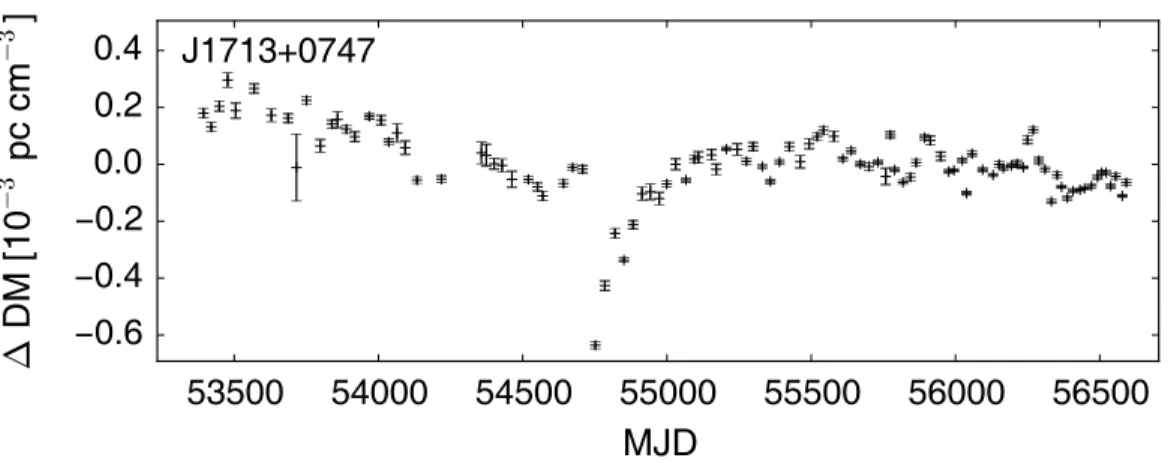
& / = − 3 R E E O − 3 ? ,

Figure 1.10 DM variations for PSR J1713+0747. Not only does the DM exhibit periodic structure, a significant dip in DM can be seen near the end of 2008 (MJD ∼54700). DM variations are discussed more throughly in Chapter 2. Data taken from the NANOGrav 9-year data release (Arzoumanian et al., 2015).

or in sharp peaks as the LOS crosses the solar ionosphere. Studying structure can determine whether a DM trend is due to a real astrophysical effect or due to some other noise processes. Variations can occur on timescales of a few hours to years. Accounting for this DM variation timescale is important when determining DM windows for DM correction. Knowledge of such structure is helpful in understanding the ISM. Characterizing the structure seen in these variations along with possible explanations of them are laid out in Chapter 2.

1.3.2 Scattering

Pulses are scattered by irregularities in the ISM, causing variable path lengths and therefore varying time delays. This results in a scatter-broadened pulse. As seen with DM, lower frequencies are more affected by the turbulent plasma in the ISM, and so low frequencies experience more scattering than higher frequencies

(31)

(scatter-Figure 1.11 Scattering of the pulse by a turbulent plasma screen sitting between the Earth and the pulsar. Image taken from Cordes (2002).

ing scales as ν−4_{, where} _ν _{is the observing frequency). Because DM and scattering}

are both frequency dependent, some scattering effects can be absorbed when fitting for DM. Low frequency observations can be used to disentangle scattering contribu-tions from DM. The same irregularities in the ISM that cause scattering also cause scintillation. As the pulse propagation paths change with time, so does the phase of the pulse when it reaches the Earth (i.e. constructive/destructive interference of the pulse). Similar to how stars twinkle when viewed from Earth, the pulse brightness will vary with the modulation of the pulse phase. The effects of scattering in pulsar timing are discussed more in Chapter 4.

1.4 Using multiple radio telescopes for GW astrophysics

There are many radio telescopes currently being used for GW detection by PTAs as well as other PTA science. Observing with multiple telescopes improves

(32)

sky coverage and cadence as multiple telescopes can observe the same source. The EPTA utilizes the Effelsberg 100-m Radio Telescope in Germany, the Lovell Telescope at Jodrell Bank in the UK, the Nan¸cay decimetric radio telescope in France, and the Westerbork Synthesis Radio Telescope in the Netherlands. When the Sardinia Radio Telescope in Italy comes fully online, it will also be used in EPTA science (Desvignes et al., 2016). This group of telescopes has the advantage of providing wide frequency coverage, high cadence, and a long timing baseline for many pulsars.

The PPTA uses the Parkes Observatory in Australia. Parkes is equipped with a 64-m dish and also has a long timing baseline for many pulsars. Parkes is able to observe MSPs in the Southern Hemisphere that are not visible to the other PTAs; this coverage is useful for the IPTA.

NANOGrav observes with the Arecibo Observatory in Puerto Rico and the Green Bank Observatory in West Virginia. The Arecibo Observatory hosts a 305-m dish; due to this large collecting area, Arecibo is extremely sensitive. Because of this size, the dish cannot move and therefore has limited range on the sky that it can observe. The Green Bank Observatory on the other hand can see ∼85% of the sky; at 100-m, it is the largest steerable object on land. Both Arecibo and Green Bank are capable of observing large bandwidths, providing the highest precision TOAs.

(33)

1.4.1 Telescopes starting to do PTA science

The Giant Metrewave Radio Telescope (GMRT) and Ooty Radio Telescope (ORT) are both part of the National Centre for Radio Astrophysics (NCRA) in India. The ORT is a 530-m long and 30-m cylindrical parabolic antenna. The GMRT is made up of 30 45-m dishes and offers frequency coverage from 150 to 1500 MHz. This lower coverage will make the GMRT useful for noise and ISM studies. The Very Large Array (VLA) in New Mexico is comprised of 27 25-m dishes. Pulsar timing has been done at the VLA for the past few years; the VLA can observe PSR J0437–4715 in the south, which is a particularly bright MSP with high timing precision. The array can also observe at high frequencies (2 to 4 GHz) which is useful for ISM mitigation. The MeerKAT radio telescope is currently operating and will be made up of 64 dishes that are each comprised of a 13.5-m reflector and 3.8-m subreflector. MeerKAT will make very sensitive TOA measurements, and will be capable of forming sub-arrays to observe multiple pulsars at once.

The Canadian Hydrogen Intensity Mapping Experiment (CHIME) telescope and Five-hundred-meter Aperture Spherical radio Telescope (FAST) are both in the commissioning phase and will be used to time pulsars once completed. CHIME con-sists of 4 100-m by 20-m semi-cylinders in British Columbia. The telescope cannot be steered, it observes the sky overhead as the Earth turns. CHIME can observe up to 10 pulsars simultaneously (observation duration depends on declination, MSPs may be visible for ∼10 minutes or less; Ng, 2017). CHIME will observe frequencies from 400 to 800 MHz. Daily observations with CHIME will be very useful for DM

(34)

correction and characterization. FAST in China is very similar to the Arecibo Ob-servatory, only much bigger (500-m) and can observe a larger range in declination. FAST will achieve incredibly sensitive observations of MSPs (Hobbs et al., 2014).

1.4.2 Combining timing data

There can be many difficulties in combining data from multiple telescopes as each telescope has its own aspects that may need to be taken into account. Telescope backends are also individual to the telescope and are replaced/upgraded over time, which needs to be accounted for when incorporating older data. Different obser-vatories may use different file formats, header information, and hardware/software for data acquisition. Data processing is done differently in each PTA, and timing models can vary between PTAs. For example, DM is corrected for by a different method, different timing parameters (e.g. using a solar wind model) may be used, among other others.

1.5 Astrophysics across a wide frequency range

In this thesis multiple radio observations at various frequencies between 322 MHz and 10 GHz are used to conduct astrophysical research related to GW detec-tion using PTAs. In Chapter 2, we discuss DM variadetec-tions seen in the NANOGrav 9-year data release using wideband multi-frequency observations. Specifically, we measure and analyze trends seen in the DM time series, propose sources of these trends, and identify timescales over which the DM varies beyond measurement

(35)

er-rors and therefore can no longer be considered constant. In Chapter 3, we analyze a previously published work that identifies the galaxy NGC 3115 as being an AGN potentially situated outside of the galactic photocenter. We investigate the pos-sibilities that the source is a SMBH binary or a post-merger recoiling SMBH. In Chapter 4, we compare DM measurements obtained with dual-frequency GMRT observations to those calculated in the NANOGrav 11-year data release and assess the relative precision of the GMRT DM measurements. We also examine data taken with the GMRT to identify its potential for inclusion in the IPTA. In Chapter 5, conclusions are put forth based on the works presented here and discuss avenues for future works.

(36)

Chapter 2 The NANOGrav Nine-Year Data Set:

Measurement and Analysis of Variations in Dispersion Measures

2.1 Abstract

We analyze dispersion measure (DM) variations of 37 millisecond pulsars in the nine-year North American Nanohertz Observatory for Gravitational Waves (NANOGrav) data release and constrain the sources of these variations. DM vari-ations can result from a changing distance between Earth and the pulsar, inhomo-geneities in the interstellar medium, and solar effects. Variations are signicant for nearly all pulsars, with characteristic timescales comparable to or even shorter than the average spacing between observations. Five pulsars have periodic annual varia-tions, 14 pulsars have monotonically increasing or decreasing trends, and 14 pulsars show both effects. Of the four pulsars with linear trends that have line-of-sight ve-locity measurements, three are consistent with a changing distance and require an overdensity of free electrons local to the pulsar. Several pulsars show correlations

Published as M. L . Jones et al. 2017, ApJ, 841, 125.

Contributing authors: M. A. McLaughlin, M. T. Lam, J. M. Cordes, L. Levin, S. Chatter-jee, Z. Arzoumanian, K. Crowter, P. B. Demorest, T. Dolch, J. A Ellis, R. D. Ferdman, E. Fonseca, M. E. Gonzalez, G. Jones, T. J. W. Lazio, D. J. Nice, T. T. Pennucci, S. M. Ransom, D. R. Stinebring, I. H. Stairs, K. Stovall, J. K. Swiggum, W. W. Zhu

(37)

between DM excesses and lines of sight that pass close to the Sun. Mapping of the DM variations as a function of the pulsar trajectory can identify localized interstel-lar medium features and, in one case, an upper limit to the size of the dispersing region of 4 AU. Four pulsars show roughly Kolmogorov structure functions(SFs), and another four show SFs less steep than Kolmogorov. One pulsar has too large an uncertainty to allow comparisons. We discuss explanations for apparent depar-tures from a Kolmogorov-like spectrum, and we show that the presence of other trends and localized features or gradients in the interstellar medium is the most likely cause.

2.2 Introduction

The principal goal of the North American Nanohertz Observatory for Grav-itational Waves (NANOGrav; McLaughlin, 2013) is to detect gravGrav-itational waves in the nanohertz regime of the gravitational wave spectrum using a pulsar timing array (PTA). Sensitivity improves as more millisecond pulsars (MSPs) are added to the PTA, and therefore it is essential to have as many well-timed MSPs as pos-sible (Siemens et al., 2013; Vigeland & Siemens, 2016). For every MSP, we must construct an accurate timing model that accounts for all known effects on the pul-sar times-of-arrival (TOAs) over decade timescales (Jenet et al., 2005; Cordes & Shannon, 2010). One of the parameters that must be fit in the timing model is the dispersion measure (DM; Lorimer & Kramer, 2012). As the pulsar signal travels through the interstellar medium (ISM), it encounters ionized plasma and electron

(38)

density variations along the way. The DM is the integrated column density of free electrons along the line of sight to a pulsar

DM =

Z d

0

ne(l)dl , (2.1)

where ne is the free electron density along a line of sight l and d is the pulsar distance. When the pulsar signal propagates through the ISM, interactions with these free electrons cause dispersion that is characterized by a frequency dependent time delay ∆t'4.15×106 ms×DM 1 ν2 1 − 1 ν2 2 , (2.2)

where ν1 and ν2 are two different frequencies in MHz and DM is in pc cm−3.

Ob-serving at least two frequencies is necessary to solve for the DM for a measured time delay. This time delay can be significant when compared to the pulsar period, and therefore the DM must be fit when creating a timing model and corrected for at each epoch (e.g. Demorest et al., 2013; Arzoumanian et al., 2015).

Inhomogeneities in the ISM, solar wind, and differences in the relative velocity of the pulsar and the Earth can change the free electron density along the line of sight (LOS; Lam et al., 2016). The result is a DM that varies with time, changing on timescales of hours to years. In this paper we discuss the variations seen in the NANOGrav 9-year data release (Arzoumanian et al., 2015), constrain the possible sources of these variations, and use these constraints to characterize the ISM along the LOS.

(39)

In §2, we discuss the data used for this analysis. In§3, we discuss the signifi-cance and trends seen in the DM time series. In §4, we perform a structure function (SF) analysis on select MSPs and put the results in the context of a Kolmogorov spectrum. In §5, we discuss the results of these analyses and in §6 we present conclusions.

2.3 The NANOGrav 9-year data set

Our analysis uses data from the NANOGrav 9-year data set (Arzoumanian et al., 2015). Pulsars were included in the data set based on the anticipated stability of their timing, their TOA precision, and their detection over a wide frequency range. Of the 37 MSPs included in the data release, 17 were reported on in Demorest et al. (2013). Observations took place roughly once a month between 2004 and 2013 with observing time spans of individual pulsars ranging from 0.6 to 9.0 years. Those MSPs with declinations between 0 and 39◦ were observed with the 305-m William E. Gordon Telescope at the Arecibo Observatory, and the rest were observed with the 100-m Robert C. Byrd Green Bank Telescope (GBT) of the National Radio Astronomy Observatory (NRAO); PSRs J1713+0747 and B1937+21 were observed with both telescopes. Every MSP was observed at multiple frequencies to account for frequency-dependent dispersion effects. Dual frequency observations occurred within ∼1 hour at Arecibo and within several days at the GBT. The typical length of an observation was ∼25 minutes. A more detailed and thorough description of these observations can be found in Arzoumanian et al. (2015).

(40)

For each pulsar, the DM was measured at nearly every observing epoch and recorded using the DMX parameter as part of the TEMPO software package1_{, where}

DMX models DM as constant over a chosen time window (14 days in this case). The ∆DM, an offset from a globally fixed fiducial DM, is fit as a free parameter in the timing model. The possible errors in DM(t) estimation using this method are discussed in Lam et al. (2015). Errors on DM are 1σ and are determined from the timing-parameter covariance matrix after the least-squares timing model fit. Data from early single-receiver observations were omitted for PSRs J1741+1351, J1853+1303, J1910+1256, J1944+0907, and B1953+29 as it was not possible to independently measure DM and other timing properties. We plot DMs vs time (i.e., DM(t)) for all of the pulsars in Figures 2.1 through 2.5. Values from the 9-year data release used in this analysis can be seen in Table 2.1. Partial DM(t) data spans have already been published for 15 pulsars (PSRs J0340+4130, J0613–0200, J1614– 2230, J1713+0747, J1738+0333, J1741+1351, J1744–1134, B1855+09, J1909–3744, J1910+1256, J1918–0642, B1937+21, J1944+0907, J2010–1323, and J2302+4442) in Levin et al. (2016).

2.4 Determining significance and trends in the variations

Variability in the DM timeseries can be seen for many pulsars; it has been a long known effect. The first detection of temporal variations was for the Crab pulsar (Rankin & Roberts, 1971). These variations were later determined to be most likely due to variations in the surrounding nebula (Isaacman & Rankin, 1977). The Vela

(41)

pulsar exhibits a decreasing time-dependent DM attributed to the pulsar motion through the enveloping supernova remnant (Hamilton et al., 1985).

We first determine whether the DM variations we see are significant or if they are consistent (within errors) with a constant DM value. We calculate the reduced χ2 _{for each pulsar as}

χ2_r = 1

NDOF

X(DM(t)−DM)2

σ(t)2 , (2.3)

where NDOF is the number of degrees of freedom, DM is the average DM value for

the data span for a pulsar (in this model), and σ(t) is the error associated with each DM(t) value. All but two of the pulsars (PSRs J1923+2515 and J2214+3000) haveχ2_r ≥1. Of these, we identify 15 pulsars as showing moderate variations (those with 1 ≤ χ2

r ≤ 10), and 20 pulsars with significant variations (χ2r ≥ 10). We therefore conclude that the DMs are intrinsically variable for all of the MSPs in our sample with the possible exceptions of J1923+2515 and J2214+3000, which both show visible variation at a low level despite the statistical test. Both of these pulsars have short data sets (2.2 and 2.1 years, respectively).

2.4.1 Systematic variations

DMs can vary in many ways, with components that appear linear, periodic, or random. Here we consider systematic DM variations such as linear trends and periodicities. Stochastic contributions are discussed in Section 2.5. Sources of linear trends and periodicities include a changing distance between the Earth and the

(42)

Table 2.1 Properties of NANOGrav MSPs in the 9-Year Data Release.

PSR µλ µβ µα µδ DM dDM dPX χ2r vT

(mas yr−1₎ _{(mas yr}−1₎ _{(mas yr}−1₎ _{(mas yr}−1₎ _{(pc cm}−3₎ _(kpc) _(kpc) _{(km s}−1₎

J0023+0923 –13.9(2) –1(1) –12.3(6) –6.7(9) 14.3 0.7(2) — 4.2 46(13) J0030+0451 –5.52(1) 3.0(5) –6.3(2) 0.6(5) 4.3 0.3(1) 0.30(2) 11 8.9(7) J0340+4130 –2.4(8) –4(1) –1.3(7) –5(1) 49.6 1.7(4) — 6.8 38(12) J0613–0200 2.12(2) –10.34(4) 1.85(2) –10.39(4) 38.8 1.7(4) 1.1(2) 70 55(10) J0645+5158 2.1(1) –7.3(2) 1.4(1) –7.5(2) 18.2 0.7(2) 0.8(3) 2.7 29(11) J0931–1902 — — — — 41.5 1.8(5) — 2.2 — J1012+5307 13.9(1) –21.7(3) 2.5(2) –25.6(2) 9.0 0.4(1) — 1.8 49(12) J1024–0719 –14.36(6) –57.8(3) –35.2(1) –48.0(2) 6.5 0.4(1) — 15 113(28) J1455–3330 8.16(7) 0.5(3) 7.9(1) –2.0(3) 13.6 0.5(1) — 2.4 19(4) J1600–3053 0.47(2) –7.0(1) –0.95(3) –7.0(1) 52.3 1.6(4) 3.0(8) 42 100(27) J1614–2230 9.46(2) –31(1) 3.8(2) –32(1) 34.5 1.3(3) 0.65(5) 20 100(8) J1640+2224 4.20(1) –10.73(2) 2.09(1) –11.33(2) 18.5 1.2(3) — 295 66(16) J1643–1224 5.56(8) 5.3(5) 6.2(1) 4.5(5) 62.4 2.3(6) — 112 84(22) J1713+0747 5.260(2) –3.442(5) 4.918(2) –3.914(5) 16.0 0.9(2) 1.18(4) 29 35(1) J1738+0333 6.6(2) 6.0(4) 6.9(2) 5.8(4) 33.8 1.4(4) — 5.0 59(17) J1741+1351 –8.8(1) –7.6(2) –9.1(1) –7.2(2) 24.2 0.9(2) — 4.7 50(11) J1744–1134 19.01(2) –8.68(8) 18.76(2) –9.20(8) 3.1 0.4(1) 0.41(2) 17 41(2) J1747–4036 0.1(8) –6(1) 0(1) –6(1) 153.0 3.3(8) — 133 — J1832–0836 — — — — 28.2 1.1(3) — 16 — J1853+1303 –1.8(2) –2.9(4) –1.48(2) –3.1(4) 30.6 2.0(5) — 5.8 32(9) B1855+09 –3.27(1) –5.10(3) –2.651(15) –5.45(3) 13.3 1.2(3) — 1335 34(9) J1903+0327 –3.5(3) –6.2(9) –2.7(3) –6.5(9) 297.6 6(2) — 27 202(71) J1909–3744 –13.868(4) –34.34(2) –9.518(4) –35.79(2) 10.4 0.5(1) 1.07(4) 1375 188(7) J1910+1256 –0.7(1) –7.2(2) 0.3(1) –7.2(2) 38.1 2.3(6) — 2.7 79(21) J1918–0642 –7.93(2) –4.85(9) –7.18(3) –5.90(9) 26.6 1.2(3) 0.9(2) 171 40(9) J1923+2515 –9.5(2) –12.8(5) –6.6(2) –14.5(5) 18.9 1.6(4) — 0.9 121(30) B1937+21 –0.02(1) –0.41(2) 0.07(1) –0.40(2) 71.0 3.6(7) — 1162 7(1) J1944+0907 9.4(1) –25.5(4) 14.37(11) –23.1(4) 24.3 1.8(5) — 147 232(64) J1949+3106 13(15) 10(13) 10(11) 13(16) 164.1 3.6(9) — 1.4 — B1953+29 –1.8(9) –4.4(14) –0.4(12) –5(1) 104.5 5(1) — 6.6 113(24) J2010–1323 1.16(4) –7.3(4) 2.71(9) –6.9(4) 22.2 1.0(3) — 70 35(11) J2017+0603 2.3(6) –0.1(7) 2.2(7) 0.5(6) 23.9 1.6(4) — 2.8 — J2043+1711 –8.97(7) –8.5(1) –5.85(7) –10.9(1) 20.7 1.7(4) 1.3(4) 6.3 100(23) J2145–0750 –12.04(4) –3.7(4) –10.1(1) –7.5(4) 9.0 0.6(2) 0.8(2) 24 48(12) J2214+3000 17.1(5) –10.5(9) 20.0(6) –1.7(8) 22.6 1.5(4) — 1.0 143(38) J2302+4442 –3.3(6) –1(2) –2(1) –3(2) 13.7 1.1(3) — 1.5 — J2317+1439 0.19(2) 3.80(7) –1.39(3) 3.55(6) 21.9 0.8(2) 1.3(4) 18732 14(4)

Notes. Columns are pulsar name, ecliptic proper motion (longitude and latitude), proper motion in RA and Dec, the DM, the DM-derived distance, the parallax-derived distance, the reduced chi-squared of the DM time series prior to any fitting, and the transverse velocity. The ecliptic proper motions and DMs were calculated for the 9-year data release (Arzoumanian et al., 2015). Proper motion in RA and Dec as well as parallax distances were calculated through timing observations and discussed in Matthews et al. (2016). The DM derived distances were calculated from the NE2001 model assuming 20% error

(Cordes & Lazio 2002). The value for χ2_r was calculated using Equation 2.3. Dashes

(43)

Table 2.2 Fitted Trends in the DM Time Series for MSPs in the 9-Year Release

PSR Trend dDM/dt Amplitude Period χ2

r PLS FAP Length δt

(10−3_{pc cm}−3_yr−1₎ ₍₁₀−4_{pc cm}−3₎ _(days) _(days) _(%) _(days) _(days)

J0023+0923 None — — — — — — 841 — J0030+0451 Periodic — 1.2(3) 373(5) 9.2 371 6.3 3204 33 J0340+4130 Linear 0.88(9) — — 1.7 241 6.3 613 73 J0645+5158 Periodic — 0.9(3) 377(29) 2.6 199 0.54 881 78 J0931–1902 None — — — — — — 235 — J1012+5307 Linear 0.11(2) — — 0.94 — — 3368 2286 J1024–0719 Linear 0.39(2) — — 2.7 — — 1467 148 J1455–3330 Linear 0.15(2) — — 1.0 361 7.3 3368 904 J1614–2230 Periodic — 3.1(5) 370(9) 11 370 0.17 1860 14 J1643–1224 Both –1.02(3) 8(1) 387(4) 10 387 0.01 3293 104 J1738+0333 Linear –0.8(2) — — 1.4 — — 1456 213 J1741+1351 Linear –0.12(4) — — 1.9 — — 1224 287 J1744–1134 Both –0.069(7) 0.4(2) 383(16) 8.0 — — 3369 66 J1747–4036 Linear –7.3(4) — — 10.0 459 6.7 608 16 J1832–0836 None — — — — — — 231 — J1853+1303 Linear 0.12(9) — — 5.2 — — 1468 361 B1855+09 Both 0.382(7) 0.5(3) 364(11) 15.7 — — 3240 27 J1903+0327 Both –3.0(4) 31(6) 375(11) 12 371 1.0 1456 99 J1909–3744 Both –0.239(4) 0.7(1) 366(5) 28 366 0.25 3306 9 J1910+1256 Linear 0.51(6) — — 0.90 404 2.9 2574 443 J1923+2515 None — — — — — — 803 — J1944+0907 Linear 1.3(2) — — 44 — — 1467 43 J1949+3106 Periodic — 10(3) 391(37) 1.0 — — 455 51 B1953+29 Both –1.3(3) 3(2) 356(72) 2.1 — — 1967 136 J2010–1323 Both 0.38(2) 2.2(4) 372(9) 14 372 0.56 1490 16 J2017+0603 Both 0.23(7) 2.3(5) 440(37) 0.94 — — 609 38 J2043+1711 Both –0.12(4) 1.0(4) 390(38) 3.7 — — 834 189 J2145–0750 Linear 0.08(2) — — 18 — — 3318 568 J2214+3000 Periodic — 4(1) 319(25) 0.83 — — 755 17 J2302+4442 Linear –0.6(2) — — 1.5 — — 613 202 J2317+1439 Both –0.550(9) 0.9(3) 311(6) 321 — — 3243 5

PSR Trend dDM/dt Amplitude Period χ2

r Start End Length δt

(10−3_{pc cm}−3_yr−1₎ ₍₁₀−4_{pc cm}−3₎ _(days) _(days) _(days)

J0613–0200 Both 0.066(7) 1.8(1) 358(4) 0.72 53448 54970 3137 18 Both 0.161(7) 1.2(2) 352(5) 3.5 54970 56380 — 23 J1600–3053 Linear –0.73(4) — — 2.8 54400 55300 2184 40 None — — — — 55300 56585 — — J1640+2224 Linear 0.145(3) — — 7.0 53344 55850 3254 78 None — — — — 55850 56599 — — J1713+0747 Both –0.066(8) 0.5(1) 400(16) 2.0 53393 54730 3199 38 None — — — — 54730 54900 — — Both –0.015(5) 0.52(9) 369(7) 5.5 54900 56592 — 26 J1918–0642 Both –0.49(1) 1.2(4) 385(11) 4.3 53292 56000 3293 24 Both 0.23(3) 1.2(3) 541(47) 2.9 56000 56585 — 31 B1937+21 Both –0.34(3) 3.2(4) 395(11) 28 53267 54550 3327 5 None — — — — 54550 55970 — — Both 0.050(3) 3.7(2) 469(14) 10 55970 56594 — 5

Notes. Results of fitting periodic and linear trends to the DM variations, where 1σ

uncertainty in the last significant digit is expressed in parentheses. The upper section lists pulsars where a single fit was applied; columns are the detected trend, the slope, the amplitude of the periodic fit, the period of the fit, the reduced chi-squared after the fitting, the period found by the Lomb-Scargle periodogram, the false alarm probability for that period, the length of the data span for that pulsar, and the average time it takes

(44)

pulsar, a wedge with linear density changes in the ISM or the orbital motion of the Earth, among others; the possible geometries from which these trends arise are explained in detail in Lam et al. (2016). Both linear and periodic trends have been seen in Parkes Pulsar Timing Array (PPTA) data (You et al., 2007; Keith et al., 2013; Petroff et al., 2013; Reardon et al., 2016). Petroff et al. (2013) determine the significance of a linear trend by calculating the error of a fit to the slope; linear trends were deemed significant if the errors are less than 35% of the slope value and highly significant if the errors on the slope measurement are less than 20%. This method is not applicable for the NANOGrav 9-year data set as a large number of pulsars exhibit sinusoidal trends without linear trends.

In order to determine the scale and structure of the variations, the options being linear, periodic, both, or variations consistent with stochastic noise, we applied a non-linear least squares fit to the data using three functions,

DM1(t) =mt +b,

DM2(t) =Acos(ωt+φ) +b,

DM3(t) =Acos(ωt+φ) +mt +b,

(2.4)

with the χ2_r calculated for the time series after each of these fits was individually subtracted off. For each fit, NDOF ≈ N − Np, where N is the number of DM measurements and Np is the number of free parameters being fit in that function (Np = 1 when DM(t) is a constant value). The threeχ2r values were then compared to the original value; the result producing the lowest χ2

(45)

The results of these fits can be seen in Table 2.2. There is a known complication when estimating the number of degrees of freedom for a non-linear model (Andrae et al., 2010). The χ2

r is only used as a metric to compare the fits of models we know to be incomplete; as stated earlier, the ISM is more complicated than a purely linear trend plus annual component. The fitting routine incorporates a non-linear least squares fit which is locally linearized around the minimum χ2

r. Later on, we describeχ2_r surfaces in the full parameter space and analyze the degree of covariance between fit parameters, finding it agrees with this fitting routine.

The periodic term in the function was fit using an initial guess of 365 days. Due to a change in sign of dDM/dt or the appearance/disappearance of a trend partway through the data span, PSRs J0613–0200, J1600–3053, J1640+2224, J1918–0642, and B1937+21 are not well characterized by a single fit. These MSPs were fit using piecewise functions, using the χ2_r of the fit to identify the applicable MJD range for each fit. The results of this partial fitting can be seen in Table 2.2. The fits can be seen in Figures 2.1 through 2.5. The χ2_r values listed in Table 2.2 are for the individual fit regions; these differ from the values shown in Figures 2.1 through 2.5 because those values incorporate both fits as well as any regions excluded from the fit.

We applied a Lomb-Scargle periodogram analysis to corroborate the best-fit periods, as an annual period was suggested during the trend fitting routine. The periodogram is also useful in possibly identifying non-annual periodicities (also seen in Table 2.2). This analysis is able to detect periodicities in unevenly sampled data

(46)

/,& ∆ & / = − 3R E E O − 3? ;GCT ∆ & / − D M = − 3R E E O − 3? , χ2 r /,& ∆ & / = − 3R E E O − 3? ;GCT ∆ & / − D M = − 3R E E O − 3? , χ2 r χ2 r /,& ∆ & / = − 3R E E O − 3? ;GCT ∆ & / − D M = − 3R E E O − 3? , χ2 r χ2 r /,& ∆ & / = − 3RE E O − 3? ;GCT ∆ & / − D M = − 3R E E O − 3? ,− χ2 r χ2 r /,& ∆ & / = − 3R E E O − 3? ;GCT ∆ & / − D M = − 3R E E O − 3? , χ2 r χ2 r /,& ∆ & / = − 3R E E O − 3? ;GCT ∆ & / − D M = − 3R E E O − 3? ,− χ2 r /,& ∆ & / = − 3R E E O − 3? ;GCT ∆ & / − D M = − 3R E E O − 3? , χ2 r χ2 r /,& ∆ & / = − 3R E E O − 3? ;GCT ∆ & / − D M = − 3R E E O − 3? ,− χ2 r χ2 r

Figure 2.1 The top panel shows the DM time series with the best fit function (if applicable) in blue. The bottom panel shows the DM residuals after the trend has been removed from the time series; an empty panel means no trend was found. The χ2

r values before and after these fits for each pulsar appear in the top and bottom panels respectively, as well as in Tables 2.1 and 2.2. PSR J0931–1902 has too short a data span for a trend to be determined.

(47)

/,& ∆ & / = − 3R E E O − 3? ;GCT ∆ & / − D M = − 3R E E O − 3? ,− χ2 r χ2 r /,& ∆ & / = − 3R E E O − 3? ;GCT ∆ & / − D M = − 3R E E O − 3? ,− χ2 r χ2 r /,& ∆ & / = − 3R E E O − 3? ;GCT ∆ & / − D M = − 3R E E O − 3? ,− χ2 r χ2 r /,& ∆ & / = − 3R E E O − 3? ;GCT ∆ & / − D M = − 3R E E O − 3? , χ2 r χ2 r /,& ∆ & / = − 3R E E O − 3? ;GCT ∆ & / − D M = − 3R E E O − 3? ,− χ2 r χ2 r /,& ∆ & / = − 3RE E O − 3? ;GCT ∆ & / − D M = − 3R E E O − 3? , χ2 r χ2 r /,& ∆ & / = − 3R E E O − 3? ;GCT ∆ & / − D M = − 3R E E O − 3? , χ2 r χ2 r /,& ∆ & / = − 3R E E O − 3? ;GCT ∆ & / − D M = − 3R E E O − 3? , χ2 r χ2 r

Figure 2.2 The top panel shows the DM time series with the best fit function (if applicable) in blue. The bottom panel shows the DM residuals after the trend has been removed from the time series; an empty panel means no trend was found. PSRs J1600–3053 and J1640+2224 were not found to have significant trends in the later parts of the DM time series.

(48)

/,& ∆ & / = − 3R E E O − 3? ;GCT ∆ & / − D M = − 3R E E O − 3? ,− χ2 r χ2 r /,& ∆ & / = − 3R E E O − 3? ;GCT ∆ & / − D M = − 3R E E O − 3? ,− χ2 r χ2 r /,& ∆ & / = − 3R E E O − 3? ;GCT ∆ & / − D M = − 3R E E O − 3? ,− χ2 r /,& ∆ & / = − 3R E E O − 3? ;GCT ∆ & / − D M = − 3R E E O − 3? , χ2 r χ2 r /,& ∆ & / = − 3R E E O − 3? ;GCT ∆ & / − D M = − 3R E E O − 3? $ χ2 r χ2 r /,& ∆ & / = − 3R E E O − 3? ;GCT ∆ & / − D M = − 3R E E O − 3? , χ2 r χ2 r /,& ∆ & / = − 3R E E O − 3? ;GCT ∆ & / − D M = − 3R E E O − 3? ,− χ2 r χ2 r /,& ∆ & / = − 3R E E O − 3? ;GCT ∆ & / − D M = − 3R E E O − 3? , χ2 r χ2 r

Figure 2.3 The top panel shows the DM time series with the best fit function (if applicable) in blue. The bottom panel shows the DM residuals after the trend has been removed from the time series; an empty panel means no trend was found. PSR J1832–0836 has too short a data span for a trend to be determined.

(49)

/,& ∆ & / = − 3R E E O − 3? ;GCT ∆ & / − D M = − 3RE E O − 3? ,− χ2 r χ2 r /,& ∆ & / = − 3R E E O − 3? ;GCT ∆ & / − D M = − 3R E E O − 3? , χ2 r /,& ∆ & / = − 3R E E O − 3? ;GCT ∆ & / − D M = − 3R E E O − 3? $ χ2 r χ2 r /,& ∆ & / = − 3R E E O − 3? ;GCT ∆ & / − D M = − 3R E E O − 3? , χ2 r χ2 r /,& ∆ & / = − 3R E E O − 3? ;GCT ∆ & / − D M = − 3R E E O − 3? , χ2 r χ2 r /,& ∆ & / = − 3R E E O − 3? ;GCT ∆ & / − D M = − 3R E E O − 3? $ χ2 r χ2 r /,& ∆ & / = − 3R E E O − 3? ;GCT ∆ & / − D M = − 3R E E O − 3? ,− χ2 r χ2 r /,& ∆ & / = − 3R E E O − 3? ;GCT ∆ & / − D M = − 3R E E O − 3? , χ2 r χ2 r

Figure 2.4 The top panel shows the DM time series with the best fit function (if applicable) in blue. The bottom panel shows the DM residuals after the trend has been removed from the time series; an empty panel means no trend was found. PSR B1937+21 could not be fit with a periodic trend throughout the data set.

(50)

/,& ∆ & / = − 3R E E O − 3? ;GCT ∆ & / − D M = − 3R E E O − 3? , χ2 r χ2 r /,& ∆ & / = − 3R E E O − 3? ;GCT ∆ & / − D M = − 3R E E O − 3? ,− χ2 r χ2 r /,& ∆ & / = − 3R E E O − 3? ;GCT ∆ & / − D M = − 3R E E O − 3? , χ2 r χ2 r /,& ∆ & / = − 3R E E O − 3? ;GCT ∆ & / − D M = − 3R E E O − 3? , χ2 r χ2 r /,& ∆ & / = − 3R E E O − 3? ;GCT ∆ & / − D M = − 3R E E O − 3? , χ2 r χ2 r

Figure 2.5 The top panel shows the DM time series with the best fit function (if applicable) in blue. The bottom panel shows the DM residuals after the trend has been removed from the time series; an empty panel means no trend was found.

(51)

FAP is the likelihood that these periods would occur as a result of random white noise. We ignored periods found by the periodogram that coincided with either the length of the data set or the observing cadence. The resolution of the analysis is equal to the cadence of the observations. Any linear trend in the DM variations will mask the periodic effect, and therefore was removed from those identified to have linear effects before applying the periodogram analysis.

2.4.2 DM variation timescale

The DM value can vary on timescales of years, days, or even hours. Therefore it is important to know on what timescale this DM is accurate. The time δt for DM to change by σDM, the rms DM in the DM time series (prior to fitting any DM

trends), gives us a rough estimate for how long a single DM estimation is valid. For a linear trend σDM δt = dDM dt =m −→δt= σDM m , (2.5)

where m is the slope of the linear trend, seen also in Equation 2.4. The time associated with a periodic trend

σDM δt = dDM dt ≈Aω −→δt= σDM Aω , (2.6)

where A and ω are the amplitude and angular frequency of the periodic trend respectively. The variation time for a DM time series showing both trends combines

(52)

4#=JTU? &'%=FGI? MSPs within 10◦ 'ENKRVKENQPIKVWFG=FGI? 'ENKRVKENCVKVWFG=FGI? MSPs within 10◦

Figure 2.6 MSP positions with respect to the ecliptic, shown in RA and Dec (left) as well as ecliptic coordinates (right). In the left plot, the ecliptic is depicted by the dashed line. Sources that lie within ∼10◦ of the ecliptic are signified by triangles.

the dDM/dt components from both the periodic and linear components

σDM

δt ≈m+Aω −→δt≈

σDM

m+Aω . (2.7)

The δt values for the MSPs showing trends are seen in Tables 2.2. This δt can inform on what timescale our DM measurement is constant and the importance of observing at epochs with spacing smaller than this timescale.

2.4.3 Solar-angle correlation

Pulsars that lie close to the ecliptic (within approximately 10◦) will have their LOS pass near the Sun during Earth’s orbit. This proximity can cause a sinusoidal trend in DM variations due to the variation in ne along the LOS from the solar wind.

(53)

5WPUGRCTCVKQP=FGI? , 5WPUGRCTCVKQP=FGI? , 5WPUGRCTCVKQP=FGI? ,− 5WPUGRCTCVKQP=FGI? ,− ∆DM [10 − 3 p c cm − 3 ]

Solar Elongation (degrees)

Figure 2.7 DM variations with respect to the solar position angle. The linear trend identified for PSR J2010–1323 has been subtracted in order to better identify any correlation in the DM as a function of solar angle. Note that the two highest DM points seen for PSR J0030+0451 were omitted from the 9-year data set as outliers and are not plotted in Figure 2.1 (discussed in Section 2.4.3).

PSRs J0023+0923, J0030+0451, J1614–2230, and J2010–1323 reside close (within approximately 6.3◦, 1.5◦, 6.8◦, and 6.5◦ respectively on closest approach in the data set) to the ecliptic. The DM as a function of solar elongation angle can be seen in Figure 2.4.3. PSRs J0023+0923 and J2010–1323 show a slight peak in DM at the smallest pulsar-Sun angles. PSRs J0030+0451 and J1614–2230 show significant peaks at the minimal solar elongation angle. It should be noted that the two highest DM points for J0030+0451 were omitted from Arzoumanian et al. (2015) as outliers but were included for this portion of the analysis.

2.4.4 Pulsar trajectories

We have plotted the pulsar trajectories through the ISM as seen from Earth, color coded to signify the DM value at each epoch (Figures 2.8 through 2.11). For this, we assumed that all of the free electrons along the line of sight are sitting in

(54)

a stationary phase screen located halfway between the Earth and the pulsar. The trajectories are the projected motions of the pulsar as seen on this phase screen. Using proper motion and distance estimates with errors from the NE2001 model (Cordes & Lazio, 2002), the transverse velocity can be calculated and used to track the pulsar’s trajectory in the sky. Proper motions were taken from the data release (seen in Table 2.1). These trajectory maps can be useful in isolating features in the ISM as well as visualizing trends in the DM time series.

2.5 Structure functions

Turbulence in the ISM is typically described as having a Kolmogorov power spectrum, meaning we expect to find larger variations over longer timescales. The power spectrum used to derive the structure function has the form

P(q)∝q−β , qouter≤q ≤qinner (2.8)

where q is the reciprocal of the size scale, and β is the power spectrum exponent. A Kolmogorov medium corresponds to a β value of 11/3, while the highest value expected for turbulence in the ISM (for an inner scale shorter than 109_{m) is} _β _{= 4}

(Rickett, 1990). The outer scale is described as the size at which the ISM ceases to be homogeneous, and the inner scale is the point at which dissipation occurs in the material along the line of sight.

The DM structure function (SF) is an effective analytic tool for characterizing interstellar turbulence over various time and size scales (Rickett, 1990; Cordes et al.,

Multi-Telescope Radio Observations for Low Frequency Gravitational Wave Astrophysics

Multi-Telescope Radio Observations for Low Frequency

Multi-Telescope Radio Observations for Low Frequency

Gravitational Wave Astrophysics

Gravitational Wave Astrophysics

Multi-Telescope Radio Observations for

Low Frequency Gravitational Wave

Astrophysics

Megan L. Jones

Acknowledgements

Table of Contents

List of Tables

List of Figures

Chapter 1

Introduction

1.1

Gravitational waves

1.1.1

Gravitational multipoles

1.1.2

Sources of gravitational waves

1.2

Pulsars

1.2.1

Millisecond pulsars

1.2.2

Pulsar timing

1.2.3

Pulsar timing array

1.3

The interstellar medium

1.3.1

Dispersion

∆

1.3.2

Scattering

1.4

Using multiple radio telescopes for GW astrophysics

1.4.1

Telescopes starting to do PTA science

1.4.2

Combining timing data

1.5

Astrophysics across a wide frequency range

Chapter 2

The NANOGrav Nine-Year Data Set:

Measurement and Analysis of Variations in Dispersion Measures

2.1

Abstract

2.2

Introduction

2.3

The NANOGrav 9-year data set

2.4

Determining significance and trends in the variations

2.4.1

Systematic variations

2.4.2

DM variation timescale

2.4.3

Solar-angle correlation

2.4.4

Pulsar trajectories

2.5

Structure functions