Should Bitcoin Be Considered a Complementary Asset in a Long-Term Investment Portfolio?

(1)

Assignment name: Essay upload May_June Name: Kasper Ahnhem

Handed in: 2017-05-24 16:17 Generated at: 2017-05-29 11:07

(2)

Department of Economics

Master’s Thesis in Economics, 15 ECTS Date of seminar: 2017-05-31

Should Bitcoin Be Considered a

Complementary Asset in a Long-Term

Investment Portfolio?

Authors

Kasper Ahnhem

Linus Lindberg

Supervisor

Dag Rydorff

(3)

2

Abstract

This thesis is set out to examine the risk-adjusted performance impact of including Bitcoin in a Swedish investor’s portfolio, how the allocation of a Swedish investor’s portfolio changes

by the inclusion of Bitcoin, and if Bitcoin should be part of a Swedish investor’s portfolio

under pessimistic views. To examine these questions, we use the Sharpe ratio, Sortino ratio, Omega ratio and the Black-Litterman model. When maximizing the Sharpe ratio, Sortino ratio and Omega ratio, Bitcoin is included in the portfolio. However, Bitcoin is not part of the new portfolio suggested by the Black-Litterman model for 50 % and 35 % expected downfall, but a part of the portfolio for 10 % expected downfall.

Keywords: Bitcoin, digital currency, Sharpe ratio, Sortino ratio, Omega ratio, Black-Litterman Model, portfolio allocation

(4)

3

Acknowledgment

We wrote this thesis during the spring term of 2017 at the Economics department at Lund University. Our goal with this thesis is to contribute to the research about Bitcoin, as an asset in portfolio management.

We want to thank our supervisor Dag Rydorff, who has always been available and provided valuable feedback when we needed it the most.

2017-05-24 Lund University

(5)

4

1. Introduction

In this chapter, we present the thesis background, research questions, research question discussion, purpose, and disposition. This chapter should give the reader an insight in how the thesis is structured, what questions we want to have answered, and why our subject is of interest.

October the 31: st, 2008, a programmer or group of programmers using the pseudonym Satoshi Nakamoto posted a paper on an online discussion forum dedicated to cryptography. The paper was titled “Bitcoin P2P e-cash paper”. Three months later, the open source code that Bitcoin is based on was released, and the first decentralized digital currency had been born (Pagliery, 2014). Ever since, Bitcoin has been a hot topic in the media and investment circles; it has frequently been reported about the controversies surrounding the digital currency, but also the exceptional value increase and the following success stories (The Telegraph, 2013). Since Bitcoin started trading in 2010, the price has increased from 0.07 USD/BTC to 1 800 USD/BTC. In Sweden, Bitcoin is relatively unknown, and the trading volume is relatively low compared to other markets, like the US and the UK (Segendorf, 2014). The scope of the thesis is to investigate if Bitcoin can be a good asset for a Swedish investor to hold in his or her portfolio.

Bitcoin is described as a virtual currency scheme based on a peer-to-peer network designed similarly to the torrent client, BitTorrent (ECB, 2012). A virtual currency is a medium of exchange but intended to be used in a specific virtual community or a network of users with specific software to handle the transactions. The issuer of a virtual currency can be a non-financial corporation or a private individual, as mentioned above Bitcoin was created and is issued by, Satoshi Nakamoto. Since Bitcoin is decentralized, it is not controlled by any country or organization nor pegged to any currency. Bitcoins can be bought on special websites and are stored in a wallet (a digital wallet), and all transactions can be done anonymously (Segendorf, 2014). The price of Bitcoin is determined by supply and demand, and Bitcoin is traded 24 hours per day, and every day of the year (The Economist, 2011). In May 2017, approximately 16.4 million Bitcoins were in circulation, and the price of one Bitcoin was approximately 1800 USD, which valued the digital currency to about 29.5 billion USD (Blockchain, 2017). The Bitcoin framework is programmed so new Bitcoins are created

(8)

7 at a diminishing rate until the total amount of Bitcoins reaches 21 million in the year 2040. Bitcoins are distributed to so-called miners, who connect their computers and servers to the Bitcoin framework and thereby verify the transactions done in Bitcoin. If more people start to mine, the mathematical problems become more advanced (ECB, 2012).

An ongoing discussion is if Bitcoin is supposed to be viewed as an asset or a currency from an investor’s perspective. In the article Bitcoin, gold and the dollar – A GARCH volatility analysis written by Dyhrberg (2016 a), the author discusses the matter. Bitcoin has by economists been compared to gold, due to its many resemblances:

Firstly, even though gold has some intrinsic value, it does not justify the 1245 USD/Ounce it is valued at today. According to Dyhrberg (2016 a), Bitcoin also has some intrinsic value, but it does not justify the price of 240.5 USD/BTC, which was the value when Dyhrberg published her article.

Secondly, Bitcoin and gold are both scarce and expensive to extract, and neither of them has a nationality nor is controlled by a government. Both are mined by independent people or companies.

Thirdly, gold was also used as a medium of exchange during the gold standard (Dyhrberg, 2016 a).

Fourthly, according to Dyhrberg (2016 a) is that Bitcoin can be used as a hedge against market risk, like gold, since good and bad news does not have an asymmetric impact on the volatility of the Bitcoin returns.

On the opposite side, Whelan (2013) has argued that Bitcoin is more similar to the US dollar. According to Whelan (2013), both the dollar and Bitcoin have no, or at least limited, intrinsic value and both are used primarily as a medium of exchange. In the report by ECB (2012), they also make the argument that today it is possible to buy both virtual and real goods and services with Bitcoin, thereby it is competing with standard currencies such as the Euro, American Dollar, and Chinese Yuan.

The price of Bitcoin is extremely volatile and therefore possesses a great risk from an investment standpoint. The price fluctuations can be linked to controversies but also political decisions. In 2013, the largest Bitcoin exchange at that time, Mt. Gox, which was handling

(9)

8 over 70 % of all Bitcoin transactions abruptly closed, due to financial problems (Villar, Knight, & Wolf, 2014). It was revealed that customers had lost 750 000 Bitcoins and Mt. Gox had lost 100 000 BTC, during the time this amounted to 6 % of all the Bitcoins in circulation (Villar, Knight, & Wolf, 2014). This event caused a lot of bad press, and the price of Bitcoin crashed. Another event in 2013 which made the Bitcoin price take a big hit was when the

People’s Bank of China stopped financial institutions from handling Bitcoin. This event caused a downfall of 30 % in a couple of hours for Bitcoin (Financial Times, 2013). Bitcoin has also been linked to criminal activity due to the anonymity of Bitcoin (Segendorf, 2014).

Bitcoin is a new phenomenon, and thereby the previous research done in the area is limited. Since Bitcoin is seen as a controversial type of asset or currency, it is often overlooked in portfolio theory. The conducted research has not been focused on how the inclusion of Bitcoin will affect a portfolio, especially a general Swedish portfolio. Due to this reason, we want to investigate further how and if Bitcoin can be included in the portfolio of a Swedish investor and how the inclusion of Bitcoin would affect the allocation of the portfolio. We investigate this by utilizing different risk-adjusted methods and building portfolios.

Main research question:

“How does the inclusion of Bitcoin in the portfolio of a Swedish investor affect the portfolio’s

risk-adjusted performance?”

Sub research questions:

“How does the inclusion of Bitcoin in the Swedish portfolio affect the allocation of the assets

in the portfolio”?

“Should Bitcoin be included in the portfolio of a Swedish investor under pessimistic investor views about Bitcoin’s future value”?

The purpose of this thesis is to analyze how the inclusion of Bitcoin affects the risk-adjusted portfolio performance and how the inclusion of Bitcoin in a general Swedish portfolio affects

(10)

9 the allocation of assets. To do so, we create portfolios consisting of Bitcoin together with other different asset classes such as stocks, bonds, real estate and commodities. Based on historical returns, we then optimize these portfolios with respect to different risk-adjusted performance measures and observe the optimal allocation of assets. If Bitcoin is in the optimal portfolio, we also optimize another portfolio excluding Bitcoin and compare the characteristics of the two portfolios. We also use the Black-Litterman model to obtain the optimal portfolio allocation under pessimistic views about the future value of Bitcoin. Our main results are that Bitcoin is included in the optimum portfolios for the Sharpe, Sortino, and Omega ratios, but it is too volatile to be included in the minimum variance portfolio. Furthermore, Bitcoin does not remain in the suggested portfolio after incorporating

pessimistic views about Bitcoin’s future value using the Black-Litterman model.

The target audience for our thesis is first and foremost students studying economics and business, who are interested in receiving a deeper knowledge about Bitcoin as an investment, but also to gain a greater general knowledge about Bitcoin. Investors and people interested in financial technology could also find our thesis to be of interest.

The thesis is structured as follows. Chapter 2 describes the previous research done within Bitcoin, Chapter 3 describes the data in the thesis, Chapter 4 presents the theoretical framework and methodology, Chapter 5 gives the main results, Chapter 6 gives the analysis and Chapter 7 gives the conclusion and recommended further research.

(11)

10

2. Previous Research

In this chapter, we present previous research about the performance of Bitcoin as a financial asset.

As stated in Chapter 1, Bitcoin is a relatively new phenomenon. This is illustrated by the fact that the price data available from Coindesk, which is one of the most frequently used database in research about the price of Bitcoin, begins first in July 2010 (Coindesk, 2017). This may be one reason for the quite scarce available research about Bitcoin as an investment. Another explanation suggested by Lee (2013) is the worldview of the most enthusiastic advocates of Bitcoin being unpopular among professional economists. The small volume and value of Bitcoin in relation to the global economy is another suggested explanation (Velde, 2013) (Wu & Pandey, 2014). However, since the spike in the Bitcoin price 2013 there has been a rising interest in the Bitcoin market, and since then more studies have been conducted (Wu & Pandey, 2014). Below is a summary of the existing research that is closest to our thesis. However, these studies all have in common the perspective of an investor holding American or global assets and data beginning in 2010 when both the price of Bitcoin and the trading volume was relatively low.

Briére et. al. (2013) use a mean-variance approach to investigate the benefits from including Bitcoin in a portfolio. They add Bitcoin into portfolios with global indexes representing traditional assets such as stocks, bonds and currencies, and alternative assets such as commodities, real estate, and hedge funds. They then perform mean-variance spanning tests as proposed by Huberman and Kandel (1987) and Ferson et. al. (1993). They conclude that Bitcoin in both tests significantly spans all categories for all portfolios which implies that portfolios containing Bitcoin deliver superior mean-variance trade-offs to portfolios not including Bitcoin. When comparing equally weighted well-diversified portfolios, they find a higher Sharpe ratio and positive asymmetry in the returns in the portfolio containing Bitcoin. They also draw mean-variance frontiers with and without Bitcoin. The frontier with Bitcoin is much steeper, but the minimum variance portfolio does not include Bitcoin. This implies that the diversification potential of Bitcoin is not high enough to compensate for its high volatility to be included in the minimum variance portfolio.

(12)

11 Dyhrberg (2016 b) explores the hedging capabilities of Bitcoin against the Financial Times Stock Exchange (FTSE) index and the dollar-euro and dollar-sterling exchange rates. First, she identifies that the Bitcoin return follows an AR (1) process and that there are ARCH-effects in the residuals. To capture leverage ARCH-effects, she uses asymmetric GARCH to model the variance. To investigate the hedging capability of Bitcoin against the FTSE index, she includes current and lagged values of the FTSE index in the mean equation and draws conclusions from the sign and significance of the coefficient for the contemporaneous effect. The author uses the same approach for the exchange rates. The results indicate that Bitcoin is not correlated with the FTSE index and can therefore be used by investors to hedge some of the market risk. For the exchange rates, the estimated correlations indicate that the exchange rates positively lead the return of Bitcoin. The contemporaneous effects are positive but very small. From the GARCH model, the author concludes that Bitcoin can be used as a short-term hedge against the dollar since the contemporaneous effects on both exchange rates are insignificant but the lagged effects are positive and significant.

Wu and Pandey (2014) use data from the U.S. between 2010 and 2013 to examine how Bitcoin correlates with different asset classes and whether Bitcoin can increase the efficiency of an investor’s portfolio. They use indexes as representations for various asset classes such

as stocks, bonds, currencies, commodities, and real estate, and combine them into a portfolio together with Bitcoin. Wu and Pandey (2014) then compute optimal portfolios based on criteria such as minimum variance and maximum Sharpe, Sortino and Omega ratios and investigate the weight of Bitcoin in these optimal portfolios. They also use the Black-Litterman model to test if Bitcoin enters the optimal portfolios given pessimistic views of the future value of Bitcoin. They conclude that Bitcoin has very low or insignificant correlation with the other investment classes and therefore could serve as a potent diversifier for an investment portfolio. Furthermore, for all the optimization measures investigated, portfolio returns are higher, and the risk of incurring a loss is lower when Bitcoin is added to the portfolio. Finally, the Black-Litterman model shows that Bitcoin remains in the optimal portfolio with a weight of roughly 1,7 % even after incorporating investor views of 50 % absolute or relative underperformance of Bitcoin in the next period.

(13)

12 Eisl et. al. (2015) adopt a Conditional Value-at-Risk framework to evaluate the impact an investment in Bitcoin can have on a well-diversified portfolio. They motivate the approach with the signs of non-normality (excess kurtosis and positive skewness) observed in Bitcoin returns. By referring to Jorion (2001) and McNeil et. al. (2005), they argue that Conditional Value-at-Risk has better properties than the classic mean-variance approach when asset returns are non-normally distributed, specifically that variance is likely to underestimate potential loss resulting from additional tail risk. They assume the position of a US investor holding an internationally diversified portfolio and use data between July 2010 and April 2015 for their analysis. Based on Conditional Value-at-Risk, they compute a risk-return ratio and use this as a performance indicator, the same way the Sharpe ratio is used. Over a rolling estimation period, the authors optimize portfolios with Bitcoin and other asset classes based on this performance indicator under different constraints on the weights such as long-only, in the interval (-100 %; 100 %) or equally weighted. The performance of these portfolios over a test period is then compared to other optimized portfolios when Bitcoin is excluded. They find the mean optimal Bitcoin weight to be positive for all portfolios, and between 1,65 % and 6,65 % depending on the constraints. The risk-return ratios are higher for the portfolios including Bitcoin under all restrictions, even the equally weighted. Based on these tests, the authors conclude that Bitcoin increase both the return and the risk of a well-diversified portfolio, but its return contribution outweigh the additional risk.

(14)

13

3. Data

In this chapter, we describe how we collect the data used in the thesis. The purpose of this chapter is to give the reader an understanding of how we have collected our data, how we use the data and where the reader can retract the data used.

3.1. Assets

The data in our thesis consist of secondary data, which we gather from the software program Thomson Reuters Datastream, and later import to Excel. We use monthly data and monthly returns, by doing this we have the same time interval for all asset returns.

Our portfolios consist of the following assets:

Bitcoin: Coindesk – USD to Bitcoin (exchange rate)

The price of one Bitcoin in US Dollar obtained from Coindesk (www.coindesk.com).

Gold: Gold Bullion LBM U$/Troy Ounce

The price of one troy ounce of gold in US Dollar.

Commodities: S&P GSCI Commodity Spot

Standard and Poor’s Goldman Sachs Commodity Index is an index containing the most liquid commodity futures, making it a good proxy for a diversified commodity portfolio. (Goldman Sachs, 2017)

Real estate: NASDAQ OMX Valueguard-KTH Housing Index Sweden (HOX)

HOX is an index constructed to be a benchmark for the housing price for the private real estate house and apartment markets in Sweden. (Valueguard, 2017)

Bonds: Sweden, Government Bond Yield Index; 1-3 years and 5+ years maturities.

OMX Nordic Exchange Stockholm’s interest-rate indexes (OMRX) is a bundle of indexes constructed to show the value growth trend for a passively managed portfolio of liquid interest-bearing Swedish securities. We use two different indexes from OMRX for short bonds (1-3 years maturities) and longer bonds (5+years maturities). (Nasdaq, 2017 a)

OMXS30 (TRI): Nasdaq OMX – OMX Stockholm 30 (OMXS30)

Total Return Index for OMX Stockholm 30. OMXS30 is an index constructed of the 30 most liquid stocks on the Swedish stock exchange. (Nasdaq, 2017 b)

(15)

14 We construct portfolios based on how a Swedish private investor’s portfolio could be allocated with the assets stated above. The allocation of assets is conducted by analyzing Sparbarometern, presented by Statistics Sweden (2017) and the assets included in "The Value of Bitcoin in Enhancing the Efficiency of an Investor's portfolio” by Wu & Pandey (2014). Bitcoin, gold, and commodities are priced in USD, but real estate, bonds, and OMXS30 are priced in SEK. Since our investment perspective is from a Swedish investor, we recalculate the return for the assets priced in USD to SEK. We recalculate the assets by using the exchange rate, SEK/USD, for every monthly return. After the recalculation, all assets are priced in SEK.

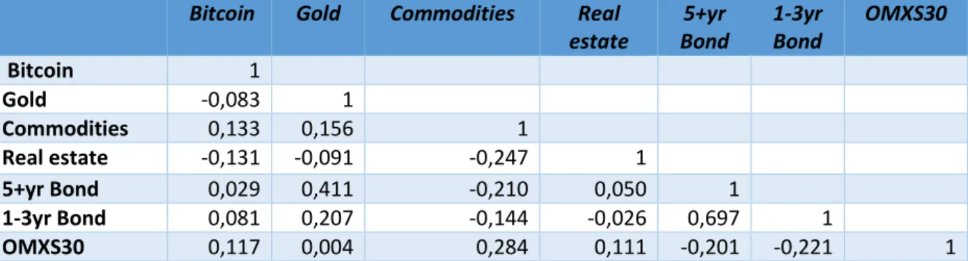
In Table 3.1 we show how the assets we choose for our portfolios correlate. Bitcoin correlates negatively with both gold and real estate, and positively with the other assets. For the assets in our sample Bitcoin correlates mostly with commodities and OMXS30.

Bitcoin Gold Commodities Real estate 5+yr Bond 1-3yr Bond OMXS30 Bitcoin 1 Gold -0,083 1 Commodities 0,133 0,156 1 Real estate -0,131 -0,091 -0,247 1 5+yr Bond 0,029 0,411 -0,210 0,050 1 1-3yr Bond 0,081 0,207 -0,144 -0,026 0,697 1 OMXS30 0,117 0,004 0,284 0,111 -0,201 -0,221 1

Table 3.1 Correlation matrix for the monthly returns of the assets used in the study

3.2. Volume

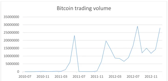
Bitcoin has actively been trading since July 2010. However, during the period between July 2010 and December 2011, the mean trading volume in Bitcoins was relatively low compared to January 2012 until April 2017. During the first period, the mean monthly trading volume was 2 155 842 Bitcoins and the second period 709 445 032 Bitcoins (Blockchain, 2017). Due to this reason, we choose to use data from January 2012 until April 2017. We base this decision on all other assets in our portfolio being liquid and the low volume in the beginning reflects that few people were buying Bitcoin. In Figure 3.1, the Bitcoin trading volume from July 2010 until January 2013 is presented to show the significant increase in volume. Due to the high price increase in Bitcoin, the actual monetary volume has also increased significantly during the period.

(16)

15

Figure 3.1 Monthly trading volume of Bitcoin between 2010-07-01 and 2013-01-01. Data source: Coindesk.com

3.3. Returns

3.3.1.Bitcoin Return

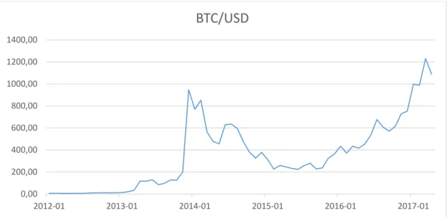
In Figure 3.2 below we present the price of Bitcoin in USD during 2012-01-01 until 2017-04-01. Since January 2012 Bitcoin has had a remarkable return, a percentage gain of 20574 %. Since the returns have been exceptionally high, we choose to separate the Bitcoin graph from the other assets. The other assets are shown in Figure 3.3. The price of Bitcoin increased substantially during the year 2013, the sudden increase in price can be linked to the banking crisis in Cyprus. When the government of Cyprus announced a bail-in for the banks, people in Cyprus ended up withdrawing funds and buying Bitcoin, which the government of Cyprus could not touch (Christensen, 2013). As shown in Figure 3.2 the Bitcoin price is extremely volatile. 0 5000000 10000000 15000000 20000000 25000000 30000000 35000000 2010-07 2010-11 2011-03 2011-07 2011-11 2012-03 2012-07 2012-11

Bitcoin trading volume

(17)

16

Figure 3.2 Bitcoin price in USD between 2012-01-01 and 2017-04-01.

3.3.2.Total Return Index

In the Figure 3.3 we compare the different assets which we use in our portfolio allocation. The comparison is made by analyzing the returns from 2012-01-01 to 2017-04-01. During this period, commodities has had the lowest return, and real estate has had the highest return of the assets excluding Bitcoin.

Figure 3.3 Total return index for Gold, Commodities, Real estate, Bonds, Stocks (left graph). Total return index for Bitcoin (right graph) 0,00 200,00 400,00 600,00 800,00 1000,00 1200,00 1400,00 2012-01 2013-01 2014-01 2015-01 2016-01 2017-01

BTC/USD

(18)

17 The data in Table 3.2 below is monthly return data for Bitcoin, gold, commodities, real estate, 1-3year bond, 5-year bond and OMXS30 from the period 2012-01-01 to 2017-04-01. We observe that Bitcoin has the highest mean, median and maximum monthly returns, but also the lowest minimum monthly return, and highest standard deviation, skewness, and kurtosis.

Bitcoin Gold Commodities Real

estate 1-3yr Bond 5+yr Bond OMXS30 Mean 0.1738 0.0007 -0.0026 0.0086 0.0008 0.0035 0.0083 Median 0.0671 -0.0014 0.0037 0.0072 0.0007 0.0028 0.0133 Maximum 3.7776 0.1351 0.1014 0.0562 0.0086 0.0504 0.0761 Minimum -0.3475 -0.1078 -0.1166 -0.0168 -0.0053 -0.0353 -0.0971 Std. Dev. 0.5910 0.0537 0.0495 0.0145 0.0024 0.0176 0.0372 Skewness 4.5048 0.2494 -0.2637 0.9882 0.1550 0.1117 -0.5378 Kurtosis 25.8871 2.7285 2.8148 4.2682 4.0544 3.0527 3.5219

(19)

18

4. Theoretical Framework and Methodology

In this chapter, we present the theoretical models and methods we use in our thesis and explain their relevance to our research questions.

4.1. Optimization Problems

To evaluate whether it is a good investment strategy to include Bitcoin in a portfolio with other asset classes, we optimize portfolios with different performance measures as targets. We then investigate if Bitcoin remains in the portfolio after the optimization procedure. If it is, we compare that portfolio with another optimized portfolio excluding Bitcoin. We rebalance the portfolio each month and restrict the portfolios to be fully invested (the asset weights sum to one) and only include long positions (all asset weights are nonnegative). We solve these optimization problems numerically using the Solver function in Excel. To reduce the risk of finding local maximum or minimum points, which are not global, we repeat the optimizations with different initial values of the weights.

4.1.1.Sharpe Ratio

The first performance measure we use to optimize the portfolio is the Sharpe ratio, a risk-adjusted performance measure developed by the Nobel Prize winner William F. Sharpe (1966). It measures the expected excess return of a portfolio or an asset per unit of risk, defined as the standard deviation.

𝑠𝑟_𝑝 =𝐸(𝑟𝑝) − 𝑟𝑓 𝜎_𝑝

Equation 1

Since the expected return is unknown, we estimate the Sharpe ratios using historical data for the portfolios: 𝑠𝑟̂ =𝑝 𝑚_𝑝 𝑠𝑝 Equation 2 where:

(20)

19 𝑚_𝑝 = 1 𝑇∑ 𝑑𝑝𝑡 𝑇 𝑡=1 𝑠𝑝= √ 1 𝑇∑(𝑑𝑝𝑡− 𝑚𝑝)2 𝑇 𝑡=1 𝑑_𝑝𝑡 = 𝑟_𝑝𝑡− 𝑟_𝑓 𝑟_𝑝𝑡= 𝑟𝑒𝑡𝑢𝑟𝑛 𝑜𝑓 𝑝𝑜𝑟𝑡𝑓𝑜𝑙𝑖𝑜 𝑝, 𝑝𝑒𝑟𝑖𝑜𝑑 𝑡 𝑟𝑓= 𝑟𝑖𝑠𝑘 𝑓𝑟𝑒𝑒 𝑟𝑒𝑡𝑢𝑟𝑛

(Jobson & Korkie, 1981)

We then solve the following maximization problem to obtain the optimal weights of the assets: max 𝑤𝑖 𝑠𝑟̂𝑝| { ∑ 𝑤𝑖 = 1 𝑤𝑖 ≥ 0 ∀ 𝑖 Equation 3

To statistically test the Sharpe ratios, we use the methods developed by Jobson and Korkie (1981). Firstly, we test if the Sharpe ratios for the optimized portfolios are significantly different from zero. A Sharpe ratio which is positive and significantly different from zero implies that investors receive compensation when taking on additional risk. We choose a one-sided alternative hypothesis since a significant negative Sharpe ratio would imply that investors pay to take on larger risks, which seems unreasonable. The assumptions behind the tests are that the portfolio returns are independent and identically distributed.

𝐻₀: 𝑠𝑟 = 0 𝐻1: 𝑠𝑟 > 0

(21)

20

𝑠𝑟̂ ~𝑁(0,1 + 1 2 𝑠𝑟̂2

𝑇 )

The test statistic is given by the estimated Sharpe ratio divided by the ratio of its standard deviation and the square root of the number of observations:

𝑧 = 𝑠𝑟̂

𝜎/√𝑇~𝑁(0,1)

Equation 4

We also examine if the difference between the Sharpe ratios of the portfolio containing Bitcoin and the portfolio excluding Bitcoin is significant. Since the portfolio excluding Bitcoin cannot have a larger Sharpe ratio (it contains the same assets but with the restriction that the Bitcoin weight is zero), the alternative hypothesis is one-sided.

𝐻0: 𝑠𝑟𝑖𝑗 ≡ 𝑠𝑟𝑖− 𝑠𝑟𝑗 = 0 𝐻₁: 𝑠𝑟_𝑖𝑗 > 0

Under H0, the difference can be transformed as follows:

𝑠𝑟̂𝑖𝑗 = 𝑠𝑟̂𝑖 − 𝑠𝑟̂𝑗 = 𝑚𝑖 𝑠𝑖 − 𝑚_𝑗 𝑠𝑗 = 𝑠𝑗𝑚𝑖 − 𝑠𝑖𝑚𝑗 Equation 5

The asymptotic distribution of the transformed difference statistic is normal with mean 𝑠𝑟_𝑖𝑗

and variance θ. 𝜃 =1 𝑇[2𝑠𝑖2𝑠𝑗2 − 2𝑠𝑖𝑠𝑗𝑠𝑖𝑗+ 1 2𝑚𝑖2𝑠𝑗2+ 1 2𝑚𝑗2𝑠𝑖2− 𝑚_𝑖𝑚_𝑗 2𝑠_𝑖𝑠_𝑗 [𝑠𝑖𝑗2 + 𝑠𝑖2𝑠𝑗2]] Equation 6

Where sij is the estimated covariance between the risk premiums of the portfolios:

𝑠_𝑖𝑗 =∑(𝑑𝑖− 𝑚𝑖) ∗ (𝑑𝑗− 𝑚𝑗) 𝑇

Equation 7

The test statistic is the estimated difference between the Sharpe ratios divided by the square root of its variance:

(22)

21

𝑧(𝑠𝑟_𝑖𝑗) =𝑠𝑟̂𝑖𝑗

√𝜃 ~𝑁(0, 1)

Equation 8

(Jobson & Korkie, 1981)

4.1.2.Sortino Ratio

The second performance measure we use to evaluate if Bitcoin should be included in an

investor’s portfolio is the Sortino ratio, introduced by Sortino and Van der Meer (1991) and Sortino and Price (1994). It measures the expected return in excess of some target rate chosen by the investor per unit of downside risk. The intuition for defining risk as the downside deviation is that if there is a minimum acceptable return (MAR), any return above the MAR is a favorable outcome. Risk is associated with bad outcomes, so volatility above the MAR should not be included in the risk measure (Sortino & van der Meer, 1991). In this subsection, we use the approach and notation described by De Capitani (2014). The formula for the Sortino ratio is given byEquation 9:

𝜐 =𝜇𝑥− 𝑘 𝜎_𝑥−_(𝑘) Equation 9 𝜎_𝑥−_{(𝑘) = (∫ (𝑥 − 𝑘)}2_𝑓 𝑥(𝑥)𝑑𝑥 𝑘 −∞ ) 1 2 where: υ = Sortino ratio

k = target return. We set this to be equal to the risk-free rate, as in Wu and Pandey (2014).

X = log-returns of the portfolio

fx = density function of X

µx = expected value of X

𝜎𝑥−(𝑘) = downside deviation

Since the expected return is unknown, we use historical data to compute the following estimator of the Sortino ratio:

(23)

22 𝜐̂ = 𝑋̅ − 𝑘 𝜎̂_𝑥−_(𝑘) Equation 10 𝑋̅ = 1 𝑛∑ 𝑋𝑖 𝑛 𝑖=1 𝜎̂𝑥−(𝑘) = ( 1 𝑛∑(𝑋𝑖 − 𝑘)2𝕀𝑘(𝑋𝑖) 𝑛 𝑖=1 ) 1 2 𝕀_𝑘(𝑋_𝑖) = { 1 𝑖𝑓 𝑋𝑖 ≤ 𝑘 0 𝑜𝑡ℎ𝑒𝑟𝑤𝑖𝑠𝑒

We then solve the following maximization problem to obtain the optimal weights of the assets: max 𝑤𝑖 𝜐̂𝑝| { ∑ 𝑤_𝑖 = 1 𝑤𝑖 ≥ 0 ∀ 𝑖 Equation 11

De Capitani (2014) presents an approach to estimate an asymptotic confidence interval for the Sortino ratio under the assumptions that the excess returns are independent and identically distributed and have a finite fourth moment. The asymptotic (1-α)-confidence interval for υ is given by Equation 12: (υ̂ − 𝑧₁₋𝛼 2 √𝑉̂𝜐 𝑛 ; υ̂ + 𝑧1−𝛼₂√𝑉 ̂_𝜐 𝑛 ) Equation 12

A consistent estimator for the variance, Vυ, is:

𝑉̂𝜐 = 𝑠2 𝜇̂₂−− ( (𝜇̂₃−_{− 𝑌̅𝜇̂} 2 −₎ (𝜇̂₂−₎3₂ ) υ̂ + ( 𝜇̂₄−_{− (𝜇̂} 2 −₎2 4(𝜇̂₂−₎2 ) υ̂2 Equation 13 where:

𝑌̅ = 𝑋̅ − 𝑘 = Average excess return

𝑠2 ₌ 1

𝑛 − 1∑(𝑌𝑖 − 𝑌̅)2 𝑛

(24)

23 𝜇_𝑗− ₌ 1 𝑛∑ 𝑌𝑖 𝑗_𝕀 0(𝑌𝑖) 𝑛 𝑖=1 with j = 2, 3, 4 𝕀₀(𝑌_𝑖) = { 1 𝑖𝑓 𝑌𝑖 ≤ 0 0 𝑜𝑡ℎ𝑒𝑟𝑤𝑖𝑠𝑒 4.1.3.Omega Ratio

The third performance measure we use is the Omega measure which was introduced by Keating and Shadwick (2002). It incorporates all higher moments of a return distribution and provides a full characterization of the risk-reward characteristics of the distribution. The only assumption behind the Omega ratio is non-satiation, which means that the investor prefers more to less. The investor must also specify a loss threshold, that is a minimum acceptable return. The Omega ratio measures the probability-weighted ratio of gains to losses relative to the minimum acceptable return, and its formula is shown in Equation 14. De Capitani (2014) shows that the Omega ratio can be rewritten as one plus the expected excess return divided by the downside mean absolute deviation, δ-.

Ω =∫ (1 − 𝐹𝑥(𝑥))𝑑𝑥 ∞ 𝑘 ∫ 𝐹_−∞𝑘 𝑥(𝑥)𝑑𝑥 = 1 +𝜇𝑥− 𝑘 𝛿𝑥−(𝑘) Equation 14 𝛿_𝑥−_{(𝑘) = ∫ |𝑥 − 𝑘|}𝑘 −∞ 𝑓_𝑥(𝑥)𝑑𝑥 Where: Ω = Omega function

X = log-returns of the portfolio

fx = density function of X

Fx = distribution function of X

µx= expected value of X

k = target return

𝛿_𝑥−_(𝑘)_{= downside mean absolute deviation (MAD)}

De Capitani (2014) derives an asymptotic confidence interval for ω, which is equal to the

Omega ratio minus one. Therefore ω is the measure we will use as well. ω can be interpreted as the downside counterpart of the MAD-ratio, as presented by Konno and Yamazaki (1991),

(25)

24 which measures the excess return per unit of risk when risk is defined as the mean absolute deviation.

𝜔 = Ω − 1 =𝜇𝑥− 𝑘 𝛿_𝑥−_(𝑘)

Equation 15

We use the following estimator of ω:

ω̂ = 𝑋̅ − 𝑘 𝛿̂_𝑥−_(𝑘) Equation 16 𝑋̅ = 1 𝑛∑ 𝑋𝑖 𝑛 𝑖=1 𝛿̂𝑥− = 1 𝑛∑(𝑘 − 𝑋𝑖)𝕀𝑘(𝑋𝑖) 𝑛 𝑖=1 𝕀_𝑘(𝑋_𝑖) = { 1 𝑖𝑓 𝑋𝑖 ≤ 𝑘 0 𝑜𝑡ℎ𝑒𝑟𝑤𝑖𝑠𝑒

We then solve the following maximization problem to obtain the optimal weights of the assets: max 𝑤𝑖 𝜔̂𝑝| { ∑ 𝑤_𝑖 = 1 𝑤_𝑖 ≥ 0 ∀ 𝑖 Equation 17

The asymptotic (1-α)-confidence interval for ω under the assumption of independently and identically distributed returns:

(ω̂ − 𝑧₁₋𝛼 2

√𝑉̂𝜔

𝑛 ; ω̂ + 𝑧1−𝛼₂√𝑉̂𝜔/𝑛)

Equation 18

(26)

25 𝑉̂𝜔 = 𝑠2 (𝜇−₎2− 2 ( 𝑌̅𝜇̂−_{− 𝜇̂} 2− (𝜇−₎2 ) 𝜔̂ + ( 𝜇̂₂−_{− (𝜇}−₎2 (𝜇−₎2 ) 𝜔̂2 Equation 19 where

𝑌̅ = 𝑋̅ − 𝑘 = Average excess return

𝜇̂− _{= −𝛿} 𝑌−(0) = −𝛿𝑋−(𝑘) 𝑠2 ₌ 1 𝑛 − 1∑(𝑌𝑖 − 𝑌̅)2 𝑛 𝑖=1 𝜇−_𝑗 = 1_𝑛∑𝑛𝑖=1𝑌_𝑖𝑗𝕀0(𝑌𝑖) with j = 2, 3, 4 𝕀0(𝑌𝑖) = { 1 𝑖𝑓 𝑌_{0 𝑜𝑡ℎ𝑒𝑟𝑤𝑖𝑠𝑒}𝑖 ≤ 0

4.1.4.Minimum Variance and Minimum Downside Variance

Finally, we follow Briére et. al. (2013) and Wu and Pandey (2014) and optimize portfolios based on risk only. As discussed in Chapter 1 and Chapter 2, Bitcoin has low correlation with both stocks and other traditional hedging assets, so as pointed out by Briére et. al (2013) and Dyhrberg (2016 b), it has high diversification potential. Therefore, it is interesting to explore if this diversification potential is enough to compensate for the high volatility by testing if Bitcoin enters the minimum variance or downside variance portfolios. To obtain the weights of the minimum variance and minimum downside variance portfolios, we solve the two minimization problems illustrated in Equation 20 and Equation 21.

min 𝑤𝑖 𝜎̂𝑝 2_{| {}∑ 𝑤𝑖 = 1 𝑤𝑖 ≥ 0 ∀ 𝑖 𝜎̂𝑝2 = 1 𝑛 − 1∑(𝑟𝑝,𝑖− 𝑟̅𝑝)2 𝑛 𝑖=1 Equation 20 min 𝑤𝑖 (𝜎̂𝑝 −_(𝑘))2_{| {}∑ 𝑤𝑖 = 1 𝑤_𝑖 ≥ 0 ∀ 𝑖

(27)

26 (𝜎̂_𝑝−_(𝑘))2 ₌ 1 𝑛 − 1∑(𝑟𝑝,𝑖− 𝑘) 2 𝕀_𝑘(𝑟_𝑝) 𝑛 𝑖=1 𝕀_𝑘(𝑟_𝑝) = { 1 𝑖𝑓 𝑟𝑝 ≤ 𝑘 0 𝑜𝑡ℎ𝑒𝑟𝑤𝑖𝑠𝑒 Equation 21

Where k is the minimum acceptable return which we set as the risk-free rate, and n is the number of observations.

(Bodie, Kane, & Marcus, 2014, ss. 132-140)

4.2. The Black-Litterman Model

Even though the historical Bitcoin returns have been high, as seen in Figure 3.3, there is no guarantee that its value will continue to increase. Following Wu and Pandey (2014), we therefore complement the backward-looking portfolio evaluation measures in Chapter 4.1 with the more forward-looking Black-Litterman model. This allows us to incorporate views of the future value of Bitcoin into a mean-variance portfolio selection model, and we can then investigate if Bitcoin remains in the portfolio even though the forecasts of its future return are more pessimistic than the historical returns.

The Black-Litterman model was introduced by Black and Litterman (1991) and expanded in Black and Litterman (1992). Its purpose is to combine a global CAPM equilibrium with views of the investor about the future returns of some of the asset classes in the portfolio. They argue that its advantages compared to standard mean-variance optimization models is that it overcomes the problems of large short position in many assets with unconstrained optimization, or corner solutions with zero weights in many assets if constraints rule out short positions. Another problem with standard asset allocation models is that they are sensitive to the expected return assumptions. Black and Litterman (1991) therefore use equilibrium risk premiums as a neutral reference point, which generates better-behaved portfolios.

The first step of the Black-Litterman model is to define a neutral reference portfolio. Black and Litterman suggest starting with the equilibrium market capitalization weighted portfolio.

(28)

27 Wu and Pandey (2014) follow their recommendation and use exchange traded funds to capture market capitalization data for the asset classes. However, Meucci (2009) states that the initial portfolio can be any reference portfolio, such as the investor’s starting portfolio or

an index. Since we in this thesis adopt the perspective of a Swedish private investor, we aim to weight the assets accordingly. To obtain these portfolio weights, we use data from Statistics Sweden (2017), which report the allocation of savings among Swedish citizens. Since Bitcoin and commodities are not included there and using the global market caps together with the allocation of the savings of only Swedish investors would be misleading, we start by using the same initial weights for those assets as Wu and Pandey (2014). These are 2,83 % for Bitcoin and 0,03 % for commodities. We then test with smaller weights for Bitcoin and observe how the results are affected.

Below we will describe how we implement the model using the approach and notation described by Idzorek (2007). N will represent the number of assets K the number of views. We only test views about Bitcoin, either absolute or relative to another asset, and we test the views separately, one view at a time. We do not incorporate any views about the individual performance of the other assets. Therefore, K is equal to one in all our tests. The equilibrium returns used in the model are obtained by a reverse optimization method in which the vector of implied excess equilibrium returns is calculated from the initial weights, the risk aversion coefficient and the covariance matrix of the returns:

Π = 𝜆Σw

Equation 22

Where Π is the implied excess equilibrium Nx1 return vector. λ is the risk aversion coefficient which characterizes the expected risk-return trade-off, that is the rate at which investors will forego expected returns for less variance. It is obtained by dividing the risk

premium by the variance of the market excess returns. Σ is the NxN covariance matrix of excess returns, which is estimated from historical returns, and w is the Nx1 vector of weights in our initial portfolio.

The Black-Litterman formula in Equation 23 generates the Nx1 vector of new combined returns, E[R]:

(29)

28

𝐸[𝑅] = [(𝜏Σ)−1_{+ 𝑃}′_Ω−1_𝑃]−1_[(𝜏Σ)−1_{Π + 𝑃}′_Ω−1_𝑄]

Equation 23

Where τ is a scalar representing the weight on views and takes on a value between 0 and 1. Meucci (2010) suggests setting τ set to 1/T, where T is the number of observations. The intuition behind this is that the views will have a higher influence when data is scarce. Π is

the Nx1 implied equilibrium return vector and Σ is the NxN covariance matrix of excess returns as described above. P is a KxN matrix that identifies the assets involved in the views. Depending on the nature of the views, the rows (each representing a view) will sum to zero if views are relative or one if views are absolute. Q is a Kx1 vector of views. We test investor views of 50 % absolute and relative underperformance, like Wu and Pandey (2014), but also with 35 %, which is the largest historical downfall in our sample period, and 10 %, which is a more likely downfall. Ω is aKxK covariance matrix of error terms from the expressed views representing the uncertainty in each view. The variance of each view is given by 𝜔_𝑘 = 𝑝_𝑘Σ𝑝_𝑘′_{, where}_p

k is the k:th row vector in the pick matrix P. If multiple views are tested

simultaneously, the model assumes that the views are independent so all off-diagonal

elements in the Ω-matrix are zero.

Ω = (

𝜔1 ⋯ 0

⋮ ⋱ ⋮

0 ⋯ 𝜔_𝑘)

The variance of the new combined return distribution is given by:

Σ_𝐵𝐿E[R] = [(𝜏Σ)−1_{+ (𝑃}′_Ω−1_𝑃)]−1

Equation 24

Σ_BL = Σ + Σ_𝐵𝐿𝐸[𝑅]

The new recommended weights in the absence of constraints are given by:

𝑤𝐵𝐿 = (𝜆ΣBL)−1Π𝐵𝐿

Equation 25

Which is the analytical solution to the following maximization problem:

max

𝑤 [𝑤´𝐸[𝑅] − 𝜆𝑤´ΣBL𝑤/2]

(30)

29 Since we want to impose short-selling constraints, we obtain the new recommended weights by solving this maximization problem numerically under long-only restrictions.

(31)

30

5. Results

In this chapter, we present the results of our portfolio optimizations described in Chapter 4 together with portfolio characteristics and the results of our statistical tests. We also present the suggested weights from the Black-Litterman model after incorporating pessimistic views about the future return of Bitcoin.

5.1. Optimization Problems

In this subsection, we describe the investor portfolios containing Bitcoin which are optimized with respect to various risk-adjusted performance measures such as the Sharpe ratio, Sortino ratio, and Omega ratio. We also provide a comparison of these portfolios with other optimized portfolios in which the Bitcoin weights are restricted to be zero. All portfolios are optimized with a short-selling constraint, and we have only considered fully invested portfolios. This means that all weights are nonnegative and the weights in all portfolios sum to one. All portfolio characteristics presented in this subsection, such as average return and volatility, are calculated on a monthly basis.

5.1.1.Sharpe Ratio

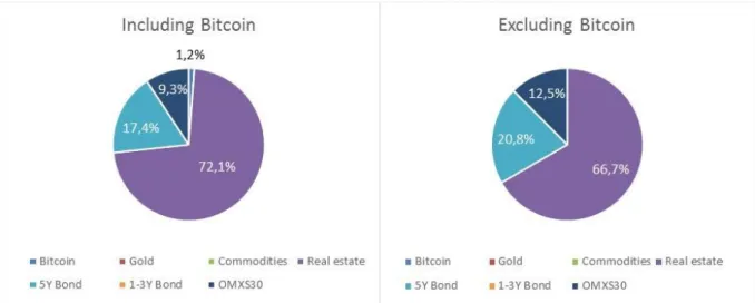
The optimal portfolio allocation with the Sharpe ratio as optimum criterion is shown in Figure 5.1 and Table 5.1.

(32)

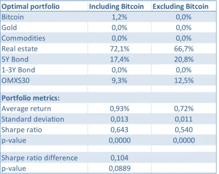
31 When we allow Bitcoin in the portfolio, its weight is 1,2 %. Gold, 1-3 year bonds, and commodities are not in the portfolio, while the weight of real estate is 72,1 %, the weight of 5-year bonds is 17,4 %, and the weight of stocks is 9,3 %. The average monthly return of this portfolio is 0,93 %, and its standard deviation is 0,013. The Sharpe ratio is 0,643 and is significantly different from zero. When we restrict the Bitcoin weight to be zero, the weight of real estate decreases to 66,7 % while the weights of 5-year bonds and stocks increase to 20,8 % and 12,5 % respectively. The weights of gold, commodities and 1-3 year bonds are still zero. The average return of this portfolio is 0,72 %, and its standard deviation is 0,011. The Sharpe ratio is 0,540 and significantly different from zero. The difference between the Sharpe ratios of the portfolios are 0,104, and the p-value of the difference is 0,0889 which is not quite significant at the five percent level.

Table 5.1 Optimal weights for portfolios with and without Bitcoin. Average monthly returns, standard deviation, Sharpe ratios and p-value for the Sharpe ratios. Difference between the Sharpe ratios of the portfolios and p-value for the difference.

Optimal portfolio Including Bitcoin Excluding Bitcoin

Bitcoin 1,2% 0,0% Gold 0,0% 0,0% Commodities 0,0% 0,0% Real estate 72,1% 66,7% 5Y Bond 17,4% 20,8% 1-3Y Bond 0,0% 0,0% OMXS30 9,3% 12,5% Portfolio metrics: Average return 0,93% 0,72% Standard deviation 0,013 0,011 Sharpe ratio 0,643 0,540 p-value 0,0000 0,0000

Sharpe ratio difference 0,104

(33)

32

5.1.2.Sortino Ratio

Figure 5.2 and Table 5.2 presents the optimal portfolios when we maximize the Sortino ratio, which is excess return per unit of downside risk.

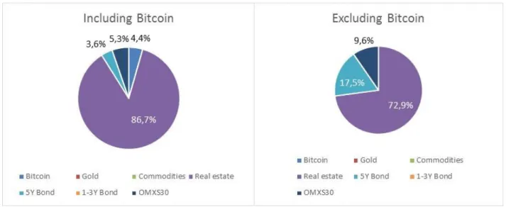
Figure 5.2 Allocation of the portfolios that maximize the Sortino ratio.

The optimal weight of Bitcoin is 4,4 %, the weight of real estate is 86,7 % the weight of 5-year bonds is 3,6 %, and the weight of stocks is 5,3 %. Commodities, Gold and 1-3 5-year bonds are not in the optimal portfolio. The average return of this portfolio is 1,48 %, and its downside deviation is 0,005. The estimated Sortino ratio is 2,89 and its 95 % confidence interval is (0,732; 5,038). When we exclude Bitcoin from the optimization, the real estate weight decrease to 72,9 % and the weight of 5-year bonds increase to 17,5 % and the weight of stocks increase to 9,6 %. Gold, commodities and 1-3 year bonds are not in this portfolio either. The average monthly return is 0,72 %, and the downside deviation is 0,004. The estimated Sortino ratio is 1,5 and its 95 % confidence interval is (0,420; 2,581). Although the point estimate of the Sortino ratio is higher when we include Bitcoin, the confidence intervals for the portfolios overlap.

(34)

33

Table 5.2 Optimal weights for portfolios with and without Bitcoin. Average monthly returns, downside deviation, Sortino ratios and 95 % confidence intervals for the Sortino ratios.

5.1.3.Omega Ratio

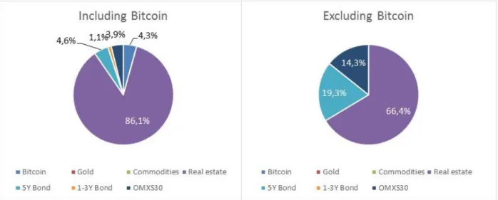
The portfolios that maximize the Omega ratio are presented in Figure 5.3 and Table 5.3.

Figure 5.3 Allocation of the portfolios that maximize the Omega ratio.

When Bitcoin is considered, its weight is 4,3 %. As in the cases when the Sharpe and Sortino ratios are maximized, gold and commodities are not in the optimal portfolio. However, 1-3 year bonds enter when we maximize the Omega ratio; its weight is 1,1 %. The weight of real estate is 86,1 %, the weight of 5-year bonds is 4,6 %, and the weight of stocks is 3,9 %. The average return of the portfolio is 1,44 %, and its downside mean absolute deviation is 0,002.

Bitcoin 4,4% 0,0% Gold 0,0% 0,0% Commodities 0,0% 0,0% Real estate 86,7% 72,9% 5Y Bond 3,6% 17,5% 1-3Y Bond 0,0% 0,0% OMXS30 5,3% 9,6% Portfolio metrics Average return 1,48% 0,72% Downside deviation 0,005 0,004 Sortino ratio 2,89 1,50 Lower CI 0,732 0,420 Upper CI 5,038 2,581

(35)

34 The point estimate of the Omega ratio is 8,783, and the 95 % confidence interval is (0,188; 17,378). Gold and commodities are not in the optimal portfolio when we exclude Bitcoin either, and the 1-3 year bonds also drops out. The weight of real estate decrease to 66,4 % and the weights of 5-year bonds and stocks increase to 19,3 % and 14,3 % respectively. The average return is 0,72 %, and the downside mean absolute deviation is 0,002. The estimated Omega ratio is 3,721 which is clearly lower than in the case when we have Bitcoin in the portfolio. However, the 95 % confidence interval is (0,239; 7,202), which is inside the confidence interval for the Bitcoin portfolio.

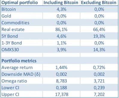
Table 5.3 Optimal weights for portfolios with and without Bitcoin. Average monthly returns, downside mean absolute deviation (MAD), Omega ratios and 95 % confidence intervals for the Omega ratios.

Optimal portfolio Including Bitcoin Excluding Bitcoin

Bitcoin 4,3% 0,0% Gold 0,0% 0,0% Commodities 0,0% 0,0% Real estate 86,1% 66,4% 5Y Bond 4,6% 19,3% 1-3Y Bond 1,1% 0,0% OMXS30 3,9% 14,3% Portfolio metrics Average return 1,44% 0,72% Downside MAD (δ) 0,002 0,002 Omega ratio 8,783 3,721 Lower CI 0,188 0,239 Upper CI 17,378 7,202

(36)

35

5.1.4.Minimum Variance and Minimum Downside Variance

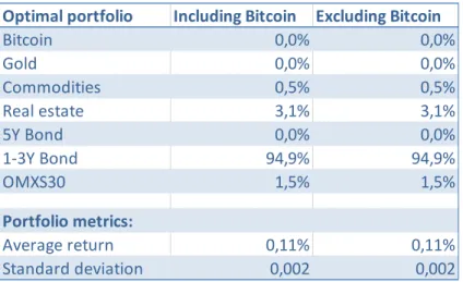
As shown in Figure 5.4 and Table 5.4, the minimum variance portfolio does not contain Bitcoin, so the two portfolios are identical in this case.

Figure 5.4 Allocation of the minimum variance portfolio.

Gold and 5-year bonds are not in the minimum variance portfolio either. The minimum variance portfolio mainly consists of 1-3 year bonds (94,9 %). The weight of commodities is 0,5 %, the weight of real estate is 3,1 %, and the weight of stocks is 1,5 %. The average return of the portfolio is 0,11 %, and its standard deviation is 0,002.

Table 5.4 Portfolio weights that minimize the variance with and without Bitcoin, average monthly return and standard deviation.

Bitcoin 0,0% 0,0% Gold 0,0% 0,0% Commodities 0,5% 0,5% Real estate 3,1% 3,1% 5Y Bond 0,0% 0,0% 1-3Y Bond 94,9% 94,9% OMXS30 1,5% 1,5% Portfolio metrics: Average return 0,11% 0,11% Standard deviation 0,002 0,002

(37)

36

Figure 5.5 Allocation of the minimum downside variance portfolios.

The minimum downside variance portfolio, on the other hand, has a small share of Bitcoin, 0,4 %, as shown in Figure 5.5 and Table 5.5. The portfolio also contains real estate (14,5 %), 1-3 year bonds (84 %) and stocks (1,1 %). Gold, commodities and 5-year bonds are not included in the portfolio. The average return of the minimum downside variance portfolio is 0,26 %, and the downside deviation is 0,0013. When we exclude Bitcoin from the portfolio, the weight of real estate decrease to 12,8 % while the weight of 1-3 year bonds increases to 85,4 % and the weight of stocks increase to 1,8 %. The average return of the portfolio is 0,18 %, and the downside deviation is 0,0014.

Table 5.5 Portfolio weights that minimize the downside variance with and without Bitcoin, average monthly return and downside deviation.

Bitcoin 0,4% 0,0% Gold 0,0% 0,0% Commodities 0,0% 0,0% Real estate 14,5% 12,8% 5Y Bond 0,0% 0,0% 1-3Y Bond 84,0% 85,4% OMXS30 1,1% 1,8% Portfolio metrics: Average return 0,26% 0,18% Downside deviation 0,0013 0,0014

(38)

37

5.1.5.Change in Weights

Figure 5.6 and Table 5.6 shows the change in the allocation of each optimum portfolio when Bitcoin is added.

Figure 5.6 Change in portfolio weights when Bitcoin is added to the portfolios.

Comparing the optimized portfolios allows us to investigate how the allocation of assets change when Bitcoin is added to the portfolio. Looking at the portfolio optimized with respect to the Sharpe ratio, we see that the weight of real estate increases to 72,1 % from 66,7 % (+5,4 %-p) when Bitcoin is added, while the weight of 5 year bonds decreases to 17,4 % from 20,8% (-3,4 %-p) and the weight of stocks decreases to 9,3 % from 12,5 % (-3,2 %-p). When the Sortino ratio is used, the weight of real estate increases to 86,7 % from 72,9 % (+13,8 %-p). The weight of 5 year bonds decreases to 3,6 % from 17,5 % (-13,9 %-p) and the weight of stocks decreases to 5,3 % from 9,6 % (-4,3 %-p). In the Bitcoin portfolio which maximizes the Omega ratio, we have 1,1 % 1-3 year bonds. They are not in the optimum portfolio without Bitcoin. For the other asset classes, we observe similar changes as when the Sharpe and Sortino ratios are used. The weight of real estate increases to 86,1 % from 66,4 % (+19,7 %-p), the weight of 5-year bonds decreases to 4,6 % from 19,3 % (-14,7 %-p) and the weight of stocks decreases to 3,9 % from 14,3 % (-10,4 %-p). Since Bitcoin is not in the minimum variance portfolio, there are no changes to that portfolio when we restrict the Bitcoin weight to be zero. In the minimum downside variance portfolio, the weight of real estate increases by 1,7 %-p from 12,8 % to 14,5 %, the weight of 1-3 year bonds decreases by 1,4 %-p from 85,4 % to 84,0 % and the weight of stocks decreases by 0,7 %-p from 1,8 % to 1,1 %.

(39)

38

Table 5.6 The change in optimal weights in percentage points when Bitcoin is included for all performance measures.

5.2. The Black-Litterman Model

In this subsection, we present the results from the forward-looking Black-Litterman model after incorporating various pessimistic views about the future return of Bitcoin. The weights are calculated under short-selling constraints and with the restriction of fully invested portfolios.

Table 5.7 shows the new recommended weights generated by the Black-Litterman model with absolute and relative views of 50 % underperformance of Bitcoin. The interpretation of the absolute view is that Bitcoin is expected to lose 50 % of its value in the next period. The interpretation of the relative views is that Bitcoin is expected to underperform with 50 % compared to some other asset in the portfolio.

Table 5.7 Initial weights and new weights suggested by the Black-Litterman model with absolute and relative views of 50 % underperformance.

Bitcoin is not included in the new recommended portfolio with the absolute view or any of the relative views of underperformance of 50 %. Using smaller initial weight for Bitcoin does not affect the results.

Real estate 5Y Bond 1-3Y Bond OMXS30

Sharpe 5,4% -3,4% 0,0% -3,2%

Sortino 13,8% -13,9% 0,0% -4,3%

Omega 19,7% -14,7% 1,1% -10,4%

Min variance 0,0% 0,0% 0,0% 0,0%

Min downside var. 1,7% 0,0% -1,4% -0,7% Change in weights (%-p)

Performance measure

Commodities Real estate 5Y Bond 1-3Y Bond OMXS30

Bitcoin 2,83% 0,00% 0,00% 0,00% 0,00% 0,00% 0,00% Commodities 0,03% 0,00% 1,63% 0,00% 0,00% 0,00% 0,00% Real estate 32,72% 50,69% 51,51% 55,45% 50,56% 50,54% 50,32% 5Y Bond 3,33% 0,00% 0,00% 0,00% 5,14% 0,00% 0,00% 1-3Y Bond 21,94% 15,94% 12,18% 11,17% 11,06% 16,19% 11,01% OMXS30 39,15% 33,37% 34,68% 33,38% 33,24% 33,27% 38,67% Initial weights

Absolute view: The value of Bitcoin decrease by 50 %

Relative view: Bitcoin will underperform the following asset class by 50 %: Optimal portfolio

(40)

39 Table 5.8 shows the new recommended weights under absolute and relative views of 35 % underperformance of Bitcoin.

Bitcoin is still not included in the new recommended portfolio with the absolute view or any of the relative views of underperformance of 35 %. Using a smaller initial weight for Bitcoin does not affect the results.

Altering the views to 10 % underperformance of Bitcoin in the next period gives the portfolios shown in Table 5.9:

In this case, a relatively small weight of Bitcoin remains in the portfolio, 0,54 % – 0,6 % depending on which asset we consider. Using a smaller initial weight for Bitcoin affects the

results in this case. With an initial equilibrium weight less than ≈1 %, Bitcoin drops out of the

portfolio. We can also see that all asset classes have weights that are closer to the initial portfolio when we have less extreme views. This is mainly because the short selling constraints do not apply in this case (all weights are positive). Relaxing these constraints with 50 % and 35 % underperformance generates portfolios that are closer to the initial portfolio but with a short position in Bitcoin.

Bitcoin 2,83% 0,00% 0,00% 0,00% 0,00% 0,00% 0,00% Commodities 0,03% 0,00% 2,07% 0,00% 0,00% 0,00% 0,00% Real estate 32,72% 42,35% 42,72% 45,42% 42,29% 42,26% 41,95% 5Y Bond 3,33% 0,95% 0,01% 0,70% 5,49% 1,29% 1,35% 1-3Y Bond 21,94% 21,00% 18,86% 18,24% 16,57% 20,79% 16,79% OMXS30 39,15% 35,70% 36,34% 35,64% 35,65% 35,66% 39,91%

Optimal portfolio Initial weights

Relative view: Bitcoin will underperform the following asset class by 35 %:

Bitcoin 2,83% 0,54% 0,55% 0,57% 0,54% 0,54% 0,60% Commodities 0,03% 0,03% 2,27% 0,03% 0,02% 0,03% 0,00% Real estate 32,72% 32,32% 32,26% 34,52% 32,27% 32,27% 32,06% 5Y Bond 3,33% 2,96% 3,15% 3,27% 5,38% 3,12% 3,13% 1-3Y Bond 21,94% 25,57% 23,22% 23,03% 23,21% 25,48% 23,46% OMXS30 39,15% 38,58% 38,55% 38,58% 38,58% 38,56% 40,75%

Optimal portfolio Initial weights

(41)

40

6. Analysis

In this chapter, we answer our research question and sub research questions by analyzing the results presented in Chapter 5. We will also embed the previous research in Chapter 2 with our results and discuss how our results cohere with the previous research about the performance of Bitcoin as a financial asset.

6.1. Main Research Question

“How does the inclusion of Bitcoin in the portfolio of a Swedish investor affect the

risk-adjusted performance?”

In the first test, we use the Sharpe ratio to obtain optimal weights, which was 1,2 % for Bitcoin. The Sharpe ratio of the portfolio is 0,643. This can be compared to 0,540 when Bitcoin is excluded. The p-value for the difference is 0,09, which is not significant at the 5 % level, but fairly close. The result implies that a Swedish investor can achieve a higher reward for taking on additional risk, defined as standard deviation, when adding Bitcoin to the portfolio. The result supports the conclusions that Bitcoin can increase portfolio efficiency by Briére et. al. (2013), but is not as convincing as in the article by Wu and Pandey (2014) in which the optimum portfolio contained 100 % Bitcoin after a similar test on the US market.

Using the Sortino ratio as optimization criteria, we find the optimal Bitcoin weight to be 4,4 %. The estimated Sortino ratio for the portfolio including Bitcoin is 2,89, compared to 1,50 when Bitcoin is excluded from the portfolio. This suggests that the risk-adjusted performance can be improved by adding Bitcoin to the portfolio also when we define risk as downside deviation. However, our estimated confidence intervals for the Sortino ratio of the two portfolios overlap, which make inference from our point estimates less reliable. Again, our results are less evidential than the results from Wu and Pandey (2014) whose optimal portfolios contained Bitcoin only.

The portfolio that maximizes the Omega ratio contains 4,3 % Bitcoin. The estimated Omega ratio is 8,783 when we include Bitcoin and 3,721 when the Bitcoin weight is set to zero. The estimates suggest that the probability-weighted ratio of gains to losses relative to our

(42)

41 minimum acceptable return (the risk-free rate), increase when Bitcoin is included in the portfolio. The estimated confidence intervals, on the other hand, are ambiguous; the interval for the Omega ratio of the portfolio excluding Bitcoin is inside the confidence interval for the Bitcoin portfolio. When Wu and Pandey (2014) perform the same optimization with assets from the US, the optimal Bitcoin weight is 9,05 %.

We believe the main reason for why Wu and Pandey (2014) obtain larger weights of Bitcoin for all three performance measures is that they use data from 2010, and thereby capture the extreme price increase during the first years Bitcoin was traded. Another possible explanation is that our results include an exchange rate effect since we convert our returns into SEK. Furthermore, it is interesting that both the Sortino ratio and the Omega ratio which both account for the additional tail risk in non-normally distributed returns give larger optimal Bitcoin weights than the Sharpe ratio. Referring to Eisl et. al. (2015), we had expected the variance to underestimate this risk and the Sharpe ratio to suggest larger weight in Bitcoin than the other two performance measures. Bitcoin is not included in the minimum variance portfolio and has only a small weight (0,4 %) in the minimum downside variance portfolio. Briére et. al. (2013) also find the volatility of Bitcoin to be too high to include it in the minimum variance portfolio, while Wu and Pandey (2014) have a small share, 0,57 % for the minimum variance and 0,25 % for the minimum downside variance, in theirs. Eisl et. al. (2015) also conclude that portfolios containing Bitcoin are riskier under the conditional value-at-risk framework than the portfolios excluding Bitcoin over the entire test period.

To summarize, the optimal portfolios include Bitcoin for all performance measures taking return into account, which suggests that Bitcoin could improve risk-adjusted performance. This is in line with previous research by Wu and Pandey (2014), Briére et. al. (2013) and Eisl et. al. (2015) on American and global portfolios. However, our statistic tests are not conclusive. When looking at risk only, Bitcoin returns are characterized by very high volatility. Bitcoin is therefore not in the minimum variance portfolio and has a very small weight (0,4 %) in the minimum downside variance portfolio, despite its diversification potential shown in previous research by Dyhberg (2016 b) or Briére et. al. (2013). We can also conclude that real estate has a large weight through all performance measures, while commodities and gold have low weights. We believe the reason for this is that real estate has

(43)

42 had low variance and high returns throughout the period, while both gold and commodities have had a very low return but also higher variance than real estate. In Table 3.2 this is presented.

6.2. Sub Research Questions

“How does the inclusion of Bitcoin in the portfolio affect the allocation of the assets in the

portfolio”?

Referring to Figure 5.6 and Table 5.6, we see that the changes in the allocation of assets when Bitcoin is added to the portfolio are quite similar for all performance measures. When Bitcoin is included, the weight of real estate increases while weights of 5-year bonds and stocks tend to decrease. The result from the Sharpe and Sortino ratio optimizations are difficult to compare with Wu and Pandey (2014) since their optimal portfolios contain 100 % Bitcoin or 100 % stocks. For the Omega ratio, the optimal weights obtained by Wu and Pandey (2014) change similarly to ours; real estate, currencies, and commodities increase, while the weight of stocks and bonds decrease. Eisl et. al. (2015) on the other hand observe the weight of bonds to increase while the weight of stocks remains roughly unchanged. They bundle the asset classes commodities, real estate, alternatives into one, which as a group decrease when Bitcoin is introduced.

“Should Bitcoin be included in the portfolio of a Swedish investor under pessimistic investor

views about its future value”?

Bitcoin is not in the new portfolio suggested by the Black-Litterman model when incorporating investor views of 50% or 35 % absolute or relative underperformance in the next period. Although it sounds intuitive that an asset which the investor expect will underperform by as much as 50 % or 35 % drops out of the portfolio, it contradicts the findings by Wu and Pandey (2014) who have roughly 1,7 % Bitcoin in all their new suggested portfolios. There are several possible explanations for this. One may be that their data set starts in the year 2010 when the price of Bitcoin was close to zero, leading to an extreme return of Bitcoin during their test period. Another reason could be that the bonds, real estate index and stock index in their portfolio are American, while ours are Swedish.

(44)

43 Furthermore, they use exchange traded funds to estimate a market cap weighted initial portfolio while we use savings data from Swedish households. With investor views of 10 % absolute or relative underperformance, we get suggested Bitcoin weights between 0,54 % and 0,60 %. However, this result depends quite heavily on the selected initial weight of Bitcoin, which is 2,8 %. If we would reduce this to roughly 1 %, Bitcoin would not remain in the portfolio. Therefore, we conclude that Bitcoin should not be included in the portfolio of a Swedish investor under pessimistic views about its future value.

(45)

44

7. Conclusion and Further Research

In this chapter, we present our conclusions for the thesis. The conclusions are reached by studying the results and the analysis. We also provide some proposals of further research in the area of Bitcoin.

The results in the thesis are fairly in line with our expectations and the previous research done in the area. While optimizing the risk-adjusted performance measures; Sharpe ratio, Sortino ratio and Omega ratio; all optimal portfolios include Bitcoin. Bitcoin has the following weights in the risk-adjusted performance measures:

Sharpe ratio – 1,2 %

Sortino ratio – 4,4 %

Omega ratio – 4,3 %

Since Bitcoin returns have a very high volatility compared to the other assets in the portfolio, Bitcoin was not included in the minimum variance portfolio and constitutes only a small weight in the minimum downside variance portfolio.

The addition of Bitcoin to the portfolios changes the allocation of assets in a similar way for all performance measures. When including Bitcoin in the portfolio, the weight of 5-year bonds and stocks decrease, while the weight of real estate increases. When examining the Black-Litterman model and incorporating negative investors views of 50% and 35% in the next period, Bitcoin is not a part of the portfolio, which contradicts the findings made by Wu and Pandey (2014). We believe the reason these results are contradicting are due to that Wu and Pandey (2014) use data from 2010, while our data starts at 2012 or that their bonds, real estate index and stock index are American while ours are Swedish. They also use exchange-traded funds, which make their portfolio allocation different from ours.

Bitcoin began trading in 2010 and is the first mainstream digital currency. Lately, Bitcoin has gained a lot of attention, and the price of Bitcoin has increased significantly. However, the research done within the area is limited. The following research would be of interest if conducted; to test if our results apply to other countries and assets, we only examine our