Wright State University Wright State University
CORE Scholar
CORE Scholar
Browse all Theses and Dissertations Theses and Dissertations 2015
Performance Prediction of Quantization Based Automatic Target
Performance Prediction of Quantization Based Automatic Target
Recognition Algorithms
Recognition Algorithms
Matthew Steven HorvathWright State University
Follow this and additional works at: https://corescholar.libraries.wright.edu/etd_all
Part of the Engineering Commons
Repository Citation Repository Citation
Horvath, Matthew Steven, "Performance Prediction of Quantization Based Automatic Target Recognition Algorithms" (2015). Browse all Theses and Dissertations. 1619.
https://corescholar.libraries.wright.edu/etd_all/1619
This Dissertation is brought to you for free and open access by the Theses and Dissertations at CORE Scholar. It has been accepted for inclusion in Browse all Theses and Dissertations by an authorized administrator of CORE Scholar. For more information, please contact [email protected].
PERFORMANCE OF QUANTIZATION BASED
AUTOMATIC TARGET RECOGNITION
ALGORITHMS
A dissertation submitted in partial fulfillment
of the requirements for the degree of
Doctor of Philosophy
by
MATTHEW S. HORVATH
B.S., The Ohio State University, 2007
M.S., Wright State University, 2011
2015
WRIGHT STATE UNIVERSITY GRADUATE SCHOOL
December 14, 2015 I HEREBY RECOMMEND THAT THE DISSERTATION PREPARED UNDER MY
SU-PERVISION BY Matthew S. Horvath ENTITLED
Performance of Quantization Based Automatic Target Recognition Algorithms BE ACCEPTED IN PARTIAL FULFILLMENT OF THE REQUIREMENTS FOR THE DEGREE OF Doctor of Philosophy
Brian D. Rigling, Ph.D. Dissertation Director
Ramana V. Grandhi, Ph.D. Director, Ph.D. in Engineering Program
Robert E. W. Fyffe, Ph.D. Vice President for Research and Dean of the Graduate School Committee on Final Examination Brian D. Rigling, Ph.D. Fred D. Garber, Ph.D. Mateen M. Rizki, Ph.D. Michael L. Raymer, Ph.D. Mark E. Oxley, Ph.D.
ABSTRACT
Horvath, Matthew S., Ph.D., Engineering Ph.D. Program, Department of Electrical Engi-neering, Wright State University, 2015. Performance of Quantization Based Automatic Target Recognition Algorithms.
The investment in and subsequent development of sensor technology has led to a glut of sensor data burdening the typically human-centric analysis and exploitation process. It is now more important than ever to have robust and well-studied automatic target recognition (ATR) algorithms to alleviate some of the burden on the human operators. The difficulty of designing these systems is that there are many sources of potential variation in the data, of-ten referred to as operating conditions (OCs) and designing algorithms robust to these OCs is difficult. Additionally, analytically determining algorithm performance, often referred to as performance prediction, as a function of these OCs is important as it provides insight into when the algorithms will fail.
Quantization based ATR algorithms have shown to be robust to certain OCs. These quantization based algorithms first discretize the pseudo-continuous data intoNq discrete
bins. This discretization step is important as it hypothetically reduces the variation due to certain nuisance parameters in the data and errors resulting from approximated signatures. This research focused on three algorithms: multinomial pattern matching (MPM), quan-tized grayscale matching (QGM), and a quanquan-tized mean-squared error approach (QMSE). The first two are known as model-based ATR algorithms and assume that in-class images are the result of realizations of a statistical model with class-conditional parametrizations. The last is a template-based algorithm which assumes a deterministic “mean” image is available with which to compare candidate targets.
The goal of this research is to develop analytic solutions, or approximations, to the per-formance of these algorithms in a process known as perper-formance prediction. This analysis shows the expected performance of these algorithms as a function of the parameters used to model the OCs, which is difficult to do with empirical simulations on even a large truthed
dataset. We focus on performance prediction approaches to a baseline AWGN noise case applicable to both SAR and EO/IR imagery, an degradation case again applicable to both SAR and EO/IR imagery, and an ideal point response case applicable to SAR imagery only, and assume that these variations are conditionally independent from other sources of variation in the data.
Abbreviations and Symbols
Throughout this dissertation numerous abbreviations and symbols are used. While the definitions can be found in surrounding text, this section provides a quick reference.
List of Abbreviations
AFRL Air Force Research Laboratory ARL Army Research Laboratory ATR Automatic Target Recognition AWGN Additive White Gaussian Noise CAD Computer Aided Design
CEM Computational Electromagnetic CFAR Constant False Alarm Rate CV Civilian Vehicle
DARPA Defense Advanced Research Projects Agency DM Dirichlet Multinomial
DMM Dirichlet Multinomial Mixture DSS Defense, Security, and Sensing EM Electromagnetic
EO Electro-optical
EOC Extended Operating Condition FOA Focus of Attention
GM Gaussian Mixture
IID Independent and Identically Distributed
IEEE Institute of Electrical and Electronics Engineers
INID Independent but Not Necessarily Identically Distributed IPR Individual Point Response
IR Infrared
KLD Kullback-Liebler Divergence MC Monte Carlo
MMSE Minimum Mean Square Error MPM Multinomial Pattern Matching MSE Mean Square Error
MSTAR Moving and Stationary Target Acquisition and Recognition OC Operating Condition
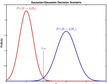
PEMS Predict, Extract, Match, and Score PTM Peaky Template Matching
QGM Quantized Grayscale Matching QMSE Quantized Mean Square Error RV Random Variable
SAIP Semi-Automated IMINT Processing SAR Synthetic Aperture Radar
SPIE International Professional Society for Optics and Photonics TAES Transactions for Aerospace and Electronic Systems
Contents
1 Introduction 1
1.1 Motivation . . . 1
1.2 Contributions . . . 6
1.2.1 GeneralNqMPM Derivation . . . 6
1.2.2 Baseline Performance Under AWGN . . . 7
1.2.3 Performance Under Target Degradation . . . 7
1.2.4 Performance Under Individual Point Response Variations . . . 8
1.3 Outline of Dissertation . . . 9
2 Literature Review 10 2.1 SAR ATR and Sensitivity Studies . . . 10
2.2 Performance Prediction . . . 14
3 The Algorithms 17 3.1 Peaky Template Matching . . . 17
3.1.1 PTM Statistical Model . . . 17
3.1.2 PTM Test Statistic and Classification Decision . . . 20
3.1.3 PTM as a Clutter Rejection Algorithm . . . 23
3.2.1 MPM Statistical Model . . . 26
3.2.2 MPM Test Statistic and Classification Decision . . . 29
3.2.3 Scalar Form of MPM Test Statistic . . . 34
3.2.4 MPM as a Clutter Rejection Algorithm . . . 36
3.3 Quantized Grayscale Matching . . . 37
3.3.1 QGM Statistical Model . . . 38
3.3.2 QGM Classification Decision . . . 42
3.4 Quantized Mean-Squared Error . . . 42
3.4.1 QMSE Statistical Model . . . 43
3.4.2 QMSE Classification Decision . . . 43
3.4.3 Chapter Summary . . . 44
4 The Datasets 46 4.1 The AFRL Civilian Vehicle Dataset for SAR . . . 46
4.2 The ARL Comanche Dataset for IR . . . 48
5 Performance Under Additive White Gaussian Noise 50 5.1 Building an Image Database . . . 51
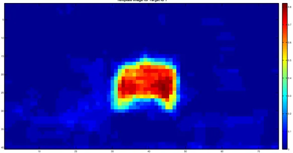
5.1.1 AFRL Civilian Vehicle Template Database . . . 52
5.1.2 ARL Comanche Template Database . . . 53
5.2 Performance Under AWGN (Nq = 2) . . . 55
5.2.1 Performance of MPM inNq = 2case . . . 56
5.2.2 Verification of Performance of MPM inNq = 2case . . . 59
5.2.3 Performance of QGM inNq = 2case . . . 61
5.2.4 Verification of Performance of QGM inNq = 2case . . . 69
5.2.5 Performance of QMSE inNq = 2case . . . 70
5.2.6 Verification of Performance of QMSE inNq = 2case . . . 75
5.3.1 Uniform Quantization and Order Statistics . . . 78
5.3.2 Verification of PTM AWGN Prediction Under Uniform Quantization 81 5.4 Performance of MPM Under AWGN in the GeneralNqCase . . . 83
5.4.1 Verification of GeneralNq Case Performance Prediction . . . 85
5.4.2 Effect of Reward Minimization on MPM . . . 86
5.5 Chapter Summary . . . 89
6 Performance Under Target Degradation 92 6.1 Image-to-Template Peformance Prediction Under Degradation . . . 94
6.1.1 A Model for Degradation . . . 94
6.1.2 Performance Analysis of MPM Under AWGN and Degradation . . 96
6.1.3 Verification Using the AFRL Civilian Vehicle Dataset . . . 100
6.2 Extension to Template-to-Template Performance Under Degradation . . . . 103
6.2.1 The Modified Degraded Model . . . 104
6.2.2 Verification Using the ARL COMANCHE Dataset . . . 105
6.3 Chapter Summary . . . 109
7 Performance Under Individual Point Response (IPR) Variations 110 7.1 General MPM Performance Prediction Approach . . . 112
7.2 Case Study Using the AFRL Civilian Vehicle Dataset . . . 113
7.2.1 Development of a Training Image Database . . . 114
7.2.2 Verification of Performance Prediction Method under IPR Variation 117 7.3 Comments and Discussion . . . 120
7.3.1 Increasing MPM’s Robustness to IPR Variations . . . 124
7.4 Chapter Summary . . . 126
8 Conclusion 129 8.1 Summary of Contributions . . . 129
8.3 Future Work . . . 132
Bibliography 133
List of Figures
1.1 A non-comprehensive list of common operating conditions . . . 2
1.2 Typical ATR classification scenario . . . 5
3.1 General representation of a training dataset . . . 18
3.2 One sided Z-test utilized by PTM and MPM . . . 22
3.3 Example QGM training scenario withN = 2training images . . . 39
3.4 Matrix encoding the likelihoods of a given QGM template . . . 40
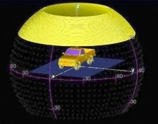
4.1 Viewing angles used in Xpatch simulations . . . 47
4.2 Statistics of available target chips from ARL Comanche dataset . . . 49
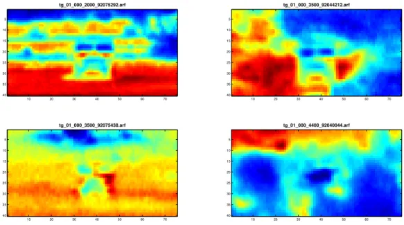
5.1 Example of original imagery and quantized representation from the AFRL CV Dome dataset . . . 53
5.2 Example of dropped chips from the ARL Comanche dataset . . . 54
5.3 Empirical probabilities for ARL Comanche target . . . 55
5.4 Illustration of the Normal/Normal decision problem . . . 57
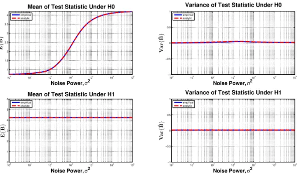
5.5 Verification of moment approximations for the CV dome Camry target us-ing PTM . . . 61
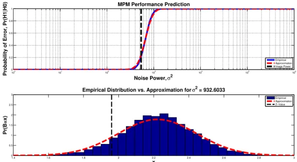
5.6 Empirical and predicted performance for the CV dome Camry target using PTM . . . 62
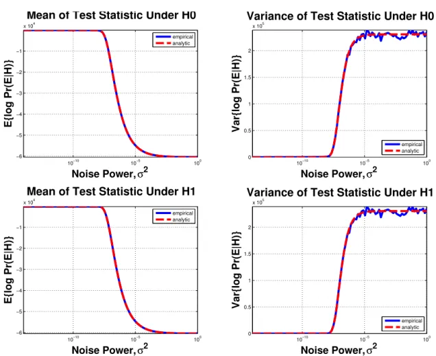
5.7 Verification of moment approximations for the CV dome Tacoma target using QGM . . . 70 5.8 Empirical and predicted performance for the CV dome Tacoma target using
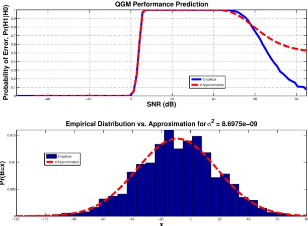
QGM . . . 71 5.9 Verification of moment approximations for the CV dome Tacoma target
using QMSE . . . 76 5.10 Empirical and predicted performance for the CV dome Tacoma target using
QMSE . . . 77 5.11 Verification of moment approximations for the CV dome Tacoma target
using PTM with uniform quantization . . . 82 5.12 Empirical and predicted performance for the CV dome Tacoma target using
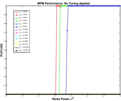
PTM with uniform quantization . . . 83 5.13 Empirical performance of MPM without clutter tuning applied . . . 88 5.14 Empirical mean shift of MPM null distribution without clutter tuning applied 89 5.15 Empirical performance of MPM with clutter tuning applied . . . 90 5.16 Empirical mean shift of MPM null distribution with clutter tuning applied . 91 6.1 Non-degraded, noise-free quantized SAR image. The pixels colored blue
are not considered by the MPM algorithm and do not exist inΓpeak. Note,
the quantized ideal sinc nature of the IPRs. . . 95 6.2 50%degraded, noise-free quantized SAR image. The pixels colored blue
are not considered by the MPM algorithm and do not exist inΓpeak. Note,
the degradation of the IPR response. . . 95 6.3 Simulated and approximated MPM distributions under AWGN and
degra-dation . . . 102 6.4 Limits of the normality assumption . . . 103 6.5 Performance prediction results under AWGN and degradation . . . 104
6.6 MSE resulting from registration in the quantized domain opposed to non-quantized . . . 106 6.7 Training dataset used for occlusion performance verification . . . 107 6.8 Moments of MPM test statistic and their approximations under degradation 108 6.9 Performance and approximated performance of MPM under degradation . . 108 7.1 Illustration of mutually exclusive decomposition scheme for 4 levels of
de-composition . . . 116 7.2 The baseline resolution image and the 4 resulting images at the first level
of decomposition . . . 117 7.3 The empirical and approximated MPM distributions at each level of
de-composition . . . 119 7.4 Performance as a function of IPR for mutually exclusive decomposition . . 120 7.5 Performance as a function of IPR for overlapping decomposition . . . 121 7.6 Illustration of recovering high resolution image from a coherent sum of
sub-band images . . . 122 7.7 Illustration of “salient” pixels included in MPM sum . . . 125 7.8 Empirical probabilities of each quantile forD= 0andD= 3decompositions127 7.9 Performance forNq = 2under IPR variations . . . 127
A.1 Verification of generalNqcase performance prediction approach shown for
Nq = 2quantization levels. . . 142
A.2 Verification of generalNqcase performance prediction approach shown for
Nq = 4quantization levels. . . 143
A.3 Verification of generalNqcase performance prediction approach shown for
Nq = 8quantization levels. . . 143
A.4 Verification of generalNqcase performance prediction approach shown for
A.5 Verification of generalNqcase performance prediction approach shown for
Nq = 32quantization levels. . . 144
A.6 Verification of generalNqcase performance prediction approach shown for
Nq = 64quantization levels. . . 145
A.7 Verification of generalNqcase performance prediction approach shown for
Nq = 128quantization levels. . . 145
A.8 Empirical and approximated performance forNq = 2quantization levels . . 146
A.9 Empirical and approximated performance forNq = 4quantization levels . . 147
A.10 Empirical and approximated performance forNq = 8quantization levels . . 148
A.11 Empirical and approximated performance forNq = 16quantization levels . 149
A.12 Empirical and approximated performance forNq = 32quantization levels . 150
A.13 Empirical and approximated performance forNq = 64quantization levels . 151
List of Tables
7.1 Number of images used for each IPR factor in experiments . . . 117 7.2 Performance equivalent SNR for each IPR factor . . . 121 8.1 A summary of contributions made by this dissertation . . . 131
Chapter 1
Introduction
1.1
Motivation
The investment in and subsequent development of sensor technology has led to a glut of sensor data burdening the typically human-centric analysis and exploitation process. Ad-ditionally, certain on-board sensors operate in time critical environments where the sensor operator is cognitively loaded with other tasks. Therefore, it is important to have robust and well-studied automatic target recognition (ATR) algorithms to alleviate some of the burden on the human operators operating in increasingly complex environments.
Designing of robust ATR systems is complicated by the many sources of potential variation in the data, often referred to as operating conditions (OCs). Additionally, analyt-ically determining algorithm performance, often referred to as performance prediction, as a function of these OCs is important as it provides insight into when the algorithms will fail. While these problems are encountered in data from all modalities, our work focuses primarily on data acquired from SAR (synthetic aperture radar) sensors, with additional studies utilizing electro-optical (EO) and infrared (IR) data.
Despite long being recognized as a problem, the formalization of the operating condi-tion or extended operating condicondi-tion (EOC) concept was the result of work in SAR ATR. A
non-comprehensive list of these OCs is shown in Figure 1.1. Certain of these OCs can be ei-ther controlled or are known a priori, typically sensor parameters and certain environmental conditions, allowing the ATR algorithm to potentially exploit this given information. Other OCs, like target pose/orientation, have to first be estimated before a classification decision is made. Still other OCs, such as configuration, occlusion, and battle damage are not known a priori, cannot typically be estimated and will degrade algorithm performance.
Figure 1.1: A non-comprehensive list of common operating conditions of interest for SAR imagery [1].
The Moving and Stationary Target Acquisition and Recognition (MSTAR) program was a joint program between the U.S. Defense Advanced Research Projects Agency (DARPA) and the U.S. Air Force Research Laboratory (AFRL) beginning in 1994, which proposed a solution to some of these difficulties [2]. While MSTAR produced a fully automated sys-tem, including target detection, constant false alarm rate (CFAR) processing, pre-screening, and classification, we focus on the classification portion that utilized a model-based pre-diction approach. This allowed signatures of likely target hypotheses be generated on the fly using a computational electromagnetic (CEM) software package. The benefits were two-fold. First, an intractably large database of signatures did not have to be maintained. Second, various OCs such as sensor resolution, imaging geometry, and background could be accounted for in the predicted signature, in addition to various target configurations. If
additional measured data was available, it could then also be used to augment the training dataset.
Despite the development of mature CEM software packages, the complexity of EM scattering still requires various approximations to be made in the predicted solution, not to mention having to rely on computer aided design (CAD) models which may not accurately model the target of interest. Additionally, radar scattering is highly sensitive to small vari-ations in aspect angle, while viewing angles are generally binned to reduce the number of simulation runs. ATR algorithms that first quantize pixel intensity values, have been shown to be robust to these concerns, and it has been hypothesized that the quantization step re-duces the sensitivity to phenomena difficult to account for when defining target type/pose representations by virtue of simply eliminating this variation from the data. These algo-rithms are referred to as quantization based algoalgo-rithms. This quantization step also reduces the complexity of the underlying statistical models, yielding models tractable to analysis as opposed to more complicated Bayesian graphical models which generally require sampling theory based simulations.
This research is a resurgence of the study of what has been termed an “ATR Theory”. The goal of “ATR Theory” is to be able to predict algorithm performance under a variety of OCs through analysis, without resorting to empirical studies of truthed datasets where fully sampling the OC space of interest is intractable [1]. In addition to an increased understand-ing of algorithm performance under operational conditions, this work can also allow for sensor optimization and higher level studies regarding how to best integrate ATR features into complex sensor systems and networks, as well as contingency planning if a primary sensor for some reason becomes unavailable and a less capable system must be utilized.
To illustrate, consider the typical ATR scenario shown in Figure 1.2. The center block is the ATR algorithm which may have some configuration variables, represented by the ‘Settings’ box, which is trained using available training data. As test data is input, the algorithm calculates a test statistic, for example a likelihood score or a mean-squared error,
which is then turned into a classification decision through a decision rule, illustrated here as a simple threshold test. Typical performance analysis of ATR algorithms involves taking an algorithm, training it with an established training dataset, then testing on a separate truthed dataset yielding an empirical performance measure.
In certain cases, a benchmark training dataset may be unavailable requiring expensive data collections to be performed. Additionally, variations in the testing data not accounted for in the training dataset will yield erroneous performance figures. Here we propose mod-elling this variation statistically, allowing an approximation to be made on the algorithm’s relevant decision statistic. In concert with the algorithm’s decision rule, this will allow for an analytic performance measure considerate of the expected variation in the data.
As the algorithms studied here are generally unstudied, even a baseline performance analysis under AWGN is a step forward. Additionally, we begin to propose simple models for variations of concern, namely a generic target degradation, which can be applicable to many scenarios like occlusion or battle damage. Cases like these are typically outside of our control, therefore they will degrade performance and the task becomes predicting and quantifying the performance loss. We finish by providing a performance prediction approach as a sensor variable changes. In this case, the variation is in our control allowing the system to be designed to optimize performance.
Our work provides both image-to-template template-to-template approaches. In the former case, the performance results are a function of an individual image’s amplitude at each pixel location and in the latter case, the performance results will be a function of pixel amplitude for each image in the training dataset. In both cases, we rely on a second-order statistical approximation to each algorithm’s decision statistic, which we show to suffi-ciently approximate the true distribution of the test statistic allowing for accurate analytic performance expressions.
Despite the origin of the OC and EOC concept in the study of SAR ATR, the goal of this work was to study performance prediction approaches of quantization based algorithms
Figure 1.2: Typical ATR classification scenario
in a generally sensor agnostic framework. It is noted that sensor specific concerns can and do arise that will naturally restrict certain performance prediction approaches to a certain sensor modality, which is the case in Chapter 7. Additionally, the statistical models used to express the OC of interest may also have sensor specific considerations. Therefore, we have opted to work with mainly SAR data, however extensions to other phenomenologies are relatively direct in most cases and are also presented.
The focus will be on three algorithms in particular: multinomial pattern matching (MPM), quantized grayscale matching (QGM), and a quantized mean-squared error ap-proach (QMSE), with the primary focus being on MPM. The first two algorithms, MPM and QGM, are known as model-based ATR algorithms and assume that in-class images are the result of realizations of a generative statistical model with class-conditional parametriza-tions. QGM is a template-based algorithm, which assumes that a deterministic “mean” image or template exists with which to compare candidate targets. As both the statistical model and “mean” image represent an algorithm’s representation of target classes, we may generally refer to both as a “templates” moving forward.
1.2
Contributions
Currently, quantization based algorithms are sparsely studied. Therefore, this is a fruitful research area with ample opportunity for original contributions. The motivation for this work has been established in the preceding section, and here, the proposed contributions will be highlighted.
1.2.1
General
Nq
MPM Derivation
To begin, the seminal reference on the MPM algorithm, is unavailable and the details need to be inferred from a pre-cursor algorithm known an peaky template matching (PTM) which is restricted to only two quantization levels (Nq = 2). Our presented derivation differs from
another available in the open literature [3] through use of a vector form interpretation of the underlying statistical model as opposed to scalar. This yields a more statistically rigorous model at the cost of a more complicated derivation and implementation. The differences between these two algorithm implementations have been studied and shown to be roughly equivalent and that the existing scalar form is preferred for reasons to be discussed. This analysis was presented in [4] and is the first proposed contribution.
Second, MPM requires a tuning procedure, as will be discussed later, in order to mini-mize erroneous classification results [5]. This tuning procedure is based on a “reward min-imization” strategy designed around ignoring background pixels that tend to be constant between target classes and can offset the mismatch between target pixels of two different classes. This process is not-optional and is required for the algorithm to work as designed. The original tuning strategy of the PTM algorithm was extended to the general Nq case,
and a specific quantization scheme was proposed. This analysis was also presented in [4] and is our second proposed contribution.
1.2.2
Baseline Performance Under AWGN
The third proposed contribution is the baseline analysis of algorithm performance under AWGN for all three algorithms: MPM, QGM, and QMSE. This analysis yields the classi-fication performance of a candidate image or target chip for a given template as a function of noise power, or alternatively SNR. The initial analysis considered only two quantization levels (Nq= 2) and was extended to the generalNqcase for MPM only. This initial
analy-sis assumed fixed quantization thresholds, and was also extended to consider an additional quantization method referred to as “uniform”. The “uniform” quantization method uses a dynamic thresholding scheme where quantile bins are determined adaptively based on the pixel values of each image.
Investigations have not yielded any published analysis on the performance for any of these algorithms under AWGN, and our analysis allows case dependent performance comparisons to be made between the three algorithms, albeit only for theNq = 2case.
The baseline AWGN analysis for all three algorithms in theNq = 2will be published
in [6]. The “uniform” quantization extension verified using IR data was presented in [7]. The extension of baseline AWGN case to the generalNqcase was also completed for MPM
and was integrated into the performance as a function of the individual point response work submitted in [8].
1.2.3
Performance Under Target Degradation
The fourth proposed contribution is the performance of the MPM algorithm under what we term “target degradation”. This is a true sensor OC of specific interest to the ATR community and one that cannot typically be accounted for using CEM simulations and therefore will yield a performance loss. Our analysis seeks to analytically predict this performance loss.
We opt for the general “target degradation” terminology to present a general approach that can be adapted to handle more specific cases of target degradation such as battle
dam-age or occlusion. In this case, certain portions of a target will be degraded according to a Dirichlet-Multinomial model, allowing an image to be classified to be modelled as a two-component mixture model. This analysis builds on the AWGN performance analysis and adds the degradation dimension parametrized by the DM parametrization and probability of degradation. This analysis also assumes the probability of degradation for each pixel is independent and identically distributed, which is a strong assumption moderated by MPM tuning rule considerations as will be discussed.
While the goal of this research is sensor agnostic performance prediction, SAR data was again used to verify the analysis. However, it is noted that this analysis can be ex-tended to EO/IR data as well, and was for the template-to-template performance under target degradation. This was was submitted in [9].
1.2.4
Performance Under Individual Point Response Variations
The fifth proposed contribution is the performance of the MPM algorithm under ideal point response (IPR) variations using SAR data. This analysis is sensor specific, as SAR is essen-tially sampling the radar cross section (RCS) of a scene in the spatial-frequency domain, and unlike the previous results can in no way be extended to the EO/IR sensor domains.
The extent of this sampling is dictated by the bandwidth of the SAR waveform and the size of the synthetic aperture, and these two parameters are effectively controlling the IPR of the resulting image. Therefore we study the ATR performance trade-offs between coherently processing a large aperture to yield a single-high resolution image as opposed to multiple sub-aperture images at lower resolutions.
As the mathematics describing this process are intractable, a comprised approach to performance prediction is proposed which can also be extended to the study of more com-plicated variations. This approach requires training MPM templates as the parameters of an OC are varied, effectively yielding samples of the performance curve as opposed to an expression for it. This work was submitted to [8].
1.3
Outline of Dissertation
The remainder of this dissertation is outlined as follows. First, the literature review is presented in Chapter 2 before the algorithm are introduced and described in Chapter 3. The datasets used to verify the performance prediction expressions are then presented in Chapter 4. The next three chapters present the performance analyses: performance under AWGN in Chapter 5, performance under degradation in Chapter 6, and performance under IPR variations in Chapter 7. Finally, the conclusions and comments on this work as a whole are presented in Chapter 8.
Chapter 2
Literature Review
The literature review for this dissertation spans a set of different topics which are orga-nized into two broad categories: SAR ATR and performance prediction. First, we will attempt to detail the historical development of SAR ATR, focusing on the published sem-inal efforts and the introduction of the OC/EOC concept. We will also discuss other ATR algorithms focusing primarily on based classification approaches. These model-based approaches assume candidate images or target chips are realizations of statistical models with class-conditional parametrizations. Lastly, we will focus on published efforts related to the performance prediction of ATR algorithms, the primary approaches taken to the problem, as well as available studies.
2.1
SAR ATR and Sensitivity Studies
Our work involves algorithms initially studied under two seminal SAR ATR efforts orig-inating from Defense Advanced Research Projects Agency (DARPA) in the mid-1990’s. One of these was the “Moving and Stationary Target Acquisition and Recognition” (MSTAR) program at the Air Force Research Laboratory and the other was the “Semi-Automated IMINT Processing” (SAIP) program at MIT Lincoln Laboratory [10] [11]. These pro-grams were broad efforts, aimed at not only the development of ATR algorithms but also
complicated implementation architectures and program management strategies, however we will focus only the aspects of the programs relevant to the research described here.
The ATR algorithm utilized in the SAIP program used a mean squared error (MSE) classifier. This approach assumes that the class-conditional references are deterministic and represented by the “average” image calculated from a training set. This is generally referred to as a template based ATR approach [12]. The class associated with the tem-plate yielding the minimum MSE score for a given candidate image is then selected by the algorithm. Novak showed this approach yielded a probability of correct identification in the high 90 percentile for both 10 and 20 target classifiers using approximately 5200 test images [13], however he also showed that the template-based approach was extremely sensitive to changes in target configuration such as additional armor-plating or fuel tanks attached to the body of the vehicle. The other notable aspect of the SAIP program was the utilization of super-resolution imaging techniques which overcome the traditional short-comings of the more efficient Fourier based processing (mainly sidelobe artifacts) at the cost of less efficient processing [14] [15]. Lastly, under a separate program the perfor-mance of the MSE algorithm as a function of resolution and polarization was also inves-tigated [16]. The performance evaluation methodology utilized in these publications was empirical and involved testing the algorithms on a sequestered portion of a training dataset. This approach has many shortcomings which we hope to demonstrate.
MSTAR differed from SAIP and in that it took a novel approach to SAR imaging based on a tenet known as model-based prediction [17] [2]. This model-based prediction approach utilizes computational electromagnetic (CEM) software packages to approximate the electromagnetic (EM) scattering and subsequent SAR signature given a computer-aided design (CAD) model of the target. This model-based was integrated into the MSTAR framework which utilized 3 stages: a focus of attention (FOA) stage, an index stage, fol-lowed finally by a predict, extract, match, and search (PEMS) stage. The FOA module is a detection stage where candidate chips are selected to be presented to the index stage at
a constant false alarm rate. The indexer can be considered a rough classification stage de-signed to select the most likely candidate hypotheses. Finally, the PEMS module iteratively searches for a final classification decision using selectively more refined target hypothe-ses. Because the signatures were generated using CEM simulation, parameters could be changed to match sensor OCs such as position, aspect, and squint and other extended op-erating conditions (EOCs) such as target configuration, articulations, and occlusions tested until the best match was found [18]. This was done in a hierarchical manner, for example first identifying the target class as a tank, then a specific model, then finally configuration and articulation. This yielded an ATR package much more robust to various OCs than the one in SAIP, however the evaluation methodology still relied on empirical simulations on a truthed dataset.
The actual ATR portion of MSTAR (the match in PEMS) is very complicated and a thorough treatment is beyond the scope of this discussion. In short, a wide variety of tech-niques and algorithms were used to calculate the match metric between candidate image or target chip and the class-conditional reference. The algorithms we are concerned with utilize what is known as the relative amplitude feature which was shown to yield acceptable performance across a wide variety of OCs [19]. This feature results from quantizing the pseudo-continuous pixel amplitude values intoNqdiscrete bins using a uniform
quantiza-tion strategy. For example, ifNq = 10bins were to be used, the lowest 1/10th of the pixel
amplitudes would receive the lowest bin quantile, the second lowest 1/10th would receive the next, and so on. This feature is preferred for one primary reason: it tends to be invariant to small errors in pose estimation and the underlying CAD model, which generally results in large variations in absolute amplitude. The quantization step simply eliminates these hypothetically small variations in the data.
One of the ATR algorithms that utilizes the relative amplitude feature is quantized grayscale matching (QGM) [5]. It is specifically designed around the MSTAR architecture in that it requires a predicted signature resulting from the model-based CAD simulation
as well as a set of in-class training images. These signatures are then used to populate a reduced multinomial model parametrized by the class-conditional maximum likelihood es-timates of pixel quantile realizations. We say reduced because the predicted signature from the MSTAR system is used to indicate which pixels are realizations of only Nq
indepen-dent underlying multinomial random variables (RVs). With the parametrized models, the likelihood of a given test image can then be calculated and the decision rule is to pick the class-conditional reference maximizing the resulting likelihood score.
Another ATR algorithm utilizing the relative amplitude feature is known as multino-mial pattern matching (MPM), also referred to as the Sandia algorithm [5]. This algorithm predates QGM and is the first example of quantized data being used in a SAR ATR con-text [5]. It is based on a pre-cursor algorithm known as peaky template matching (PTM) which can be considered a special case of the MPM algorithm with only two quantization levels (Nq = 2). We note that the seminal reference on MPM is unavailable and we must
therefore infer its contents based on existing works in the literature [3] [20] [5] which do contain a description of the algorithm implementation but little description of the under-lying model. MPM uses the same categorical/multinomial statistical model as QGM [21], however each pixel is allowed a different distribution. A Bayesian estimate of the underly-ing probabilities is then used to parametrize a Dirichlet-Multinomial model in the general
Nq case which reduces to the Beta-Bernoulli in the special case that Nq = 2. Its decision
rule is based on a test statistic designed to be standard normal under the hypothesis that the image originated from class-conditional reference distribution [22]. Unlike, QGM which picks the most likely match in the template set, MPM tests each reference distribution inde-pendently allowing for ‘unknown’ classification decisions inherently solving the open-set problem [23] [24].
We can draw distinctions between the MSE algorithm and the QGM and MPM al-gorithms in that the former is a template-based algorithm assuming the class-conditional references can be modelled with a deterministic template. The latter are model-based
ATR algorithms, not be confused with the model-based prediction approach utilized by the MSTAR framework, and assume the references are statistical models with class-conditional parametrizations.
Other model based approaches have been published, however without the quantiza-tion step. A condiquantiza-tionally Gaussian model was utilized by O’Sullivan resulting in above 90%correct identification for a simple 4 target problem, however performance did suffer under EOCs [25]. This approach was generalized by DeVore to a conditionally Rician able to handle complex pixel values which performed nearly the same as the conditionally Gaussian, however with much greater complexity [26]. Both of these approaches utilized a Bayesian approach that required first estimating target pose, generally considered a nui-sance parameter, before a classification decision could be made. In a later work, DeVore quantitatively tested other models and suggested that a quarter-power normal is perhaps the best fit to the SAR data in his experiments [27]. The conditionally Gaussian model was shown to be the most efficient in terms of complexity by Sullivan [28].
This is far from an exhaustive study of SAR ATR approaches, but they do span the subset of model-based approaches that are amenable to analytic performance prediction as will be shown below.
2.2
Performance Prediction
Some of the work in the preceding section described the performance of the algorithms. This performance is typically evaluated in an empirical manner, using the results of em-pirical simulations on a truthed dataset as absolute characterizations of their performance. Unsurprisingly, it was seen that testing the algorithms at or very near their training condi-tions yielded good classification performance, and one of the novel aspects of the MSTAR program was the idea of also testing under OCs and EOCs to more rigorously assess al-gorithm performance as described by Mossing and Ross [29]. It is note worthy they also
showed that the detection problem is typically much easier to characterize than the classi-fication problem, which makes intuitive sense.
This was definitely a step forward, however the performance evaluation methodologies still relied on empirical studies utilizing a truthed testing dataset, preferably sequestered from the algorithms developers and not contained in the training datasets. Ross et al. il-lustrated the shortcomings of this approach, namely that a true random sampling of the OC space of interest is intractable to impossible [1]; even with tens of thousands of test images there is no guarantee that the random space is adequately sampled to generalize the results of an empirical test to a rigorous assessment of algorithm performance. Further, this rigorous assessment of algorithm performance is of upmost importance when transitioning R&D level technology to an operational capacity.
Therefore, it becomes of importance to have analytical performance expressions ca-pable of predicting algorithm performance as a function of OC that can then be verified and compared with simulations involving collected or simulated data. This is generally a difficult task requiring analytically tractable models that are not always able to accurately represent real world phenomenon. This is one of the benefits of the quantization based algorithms in that the quantization step has a tendency to reduce or eliminate the variation due to certain nuisance parameters allowing the use of reduced or more tractable models for various OC phenomenology [3]. Additionally, model-based ATR algorithms are use-ful in this context as parametrized statistical models are already postulated. This allows performance prediction through a variety of means, one of which is based in information theoretic concepts, as the work of Pasala and Malas demonstrates [30] [31]. The benefit of these approaches is that bounds on classification or detection performance are known in terms of certain information theoretic quantities [32].
Another approach was utilized by Chiang who designed a feature based Bayes’ clas-sifier based on a parametric scattering features [33], which allowed performance prediction by parametrizing the distribution of each feature as Gaussian [34] under the EOCs
includ-ing resolution, statistical model mismatch, and correlated features.
Dudgeon has authored a comprehensive survey concerning the benefits and limita-tions of both Bayesian and information theoretic performance prediction approaches [35]. These approaches can be considered ‘canned’ as they generally involve stuffing an ATR problem into a mathematical vehicle with well-studied routes arriving at a final rigorous performance appraisal.
Another example of a performance prediction approach is illustrated by Irving et al. who were able to generate ROC curves of a detector using peaks extracted from the data [36]. A Poisson process was used to model both clutter and target chips allowing the parametrization of a generalized likelihood ratio test (GLRT) statistic allowing ROC curves to be generated and performance to be predicted. They key contribution here was utilizing the Poisson model which did require making some assumptions that were noted to have not been thoroughly verified. This is the approach we have chosen to follow in our research and relies more on postulating a descriptive model of the OC of interest, and expressing the associated decision statistics as a function of the OC, allowing performance metrics of interest to be analytically expressed using each algorithm’s decision rule.
Chapter 3
The Algorithms
Before moving unto the primary contributions, which involves deriving expressions de-scribing the performance of each algorithm under specific OCs (AWGN, occlusion, and IPR), the algorithms must first be introduced and described.
3.1
Peaky Template Matching
MPM and its precursor Peaky Template Matching (PTM) were developed at Sandia Na-tional Laboratories in the mid-1990s [5]. They were not initially developed for the MSTAR program, the DARPA program briefly discussed previously. However, their performance garnered attention in the ATR community. Since the algorithm’s original development, it has also been utilized for classification of 1-D high range resolution (HRR) profiles as well as applied to other sensor modalities [3] [20].
3.1.1
PTM Statistical Model
The underlying statistical model for PTM utilizes a Beta-Bernoulli model where each quan-tized pixel is a Bernoulli random variable (RV) with underlying probabilities distributed as Beta. Each pixel is assumed independent, however is allowed a different probability. This
model is a result of using a Bayesian estimate of the underlying probabilities a pixel will realize a given quantization level from a set of in-class training images. This is the special case where Nq = 2 of the more general Dirichlet-Multinomial model utilized by MPM
described in Section 3.2.
To illustrate, consider Figure 3.1 where we depict a dataset ofN quantized images of the same type/pose class label comprised of K pixels each. As each image is quantized to Nq = 2 values, the entries of the dataset can take on values in the set {0,1}. PTM
assumes that each column is an independent and identically distributed (IID) realization of theK independent but not necessarily identically distributed (INID) underlying Bernoulli RVs. These realizations are then used to estimate the probabilitypiof each pixel/RV using
a Bayesian approach. This process defines the class-conditional reference distribution and is effectively training the algorithm.
Figure 3.1: General representation of a training dataset, Ii(n) = q, i ∈ [1. . . K], n ∈
[1. . . N],q∈[1. . . Nq].
The likelihood of a sequence of IID Bernoulli realizations (each column of Figure 3.1) can be written as Pr(Ii|pi) = p N1 i i (1−pi)N 0 i (3.1) where N1 i = PN
n=1Ii(n), i.e. the count of images with a value of 1 at pixel location i
over the number of images training images,N, and similiarly forN0
i except it is a count of
posterior Pr(pi|Ii)using Baye’s method with conjugate priors. The prior Beta distribution
can be written as
Pr(pi|α0, α1) =pα1
−1
i (1−pi)α0−1 ∼Beta{α0, α1} (3.2)
up to a constant term consisting of a ratio of gamma functions. Then, α0 andα1 can be
interpreted as virtual counts of 1’s or 0’s capable of encoding any a priori information on the underlying probability. The developers of MPM chose a non-informative prior,(α0, α1) =
(1,1), typically known as Laplace’s prior. It can then be shown that by conditioning on the set of theN training images [37], the posterior distribution becomes
Pr(pi|Ii) = p N1 i i (1−pi)N 0 i (3.3)
up to a constant and with (α0, α1) = (1,1), known to be Beta distributed yielding the
Beta-Bernoulli model where
Xi ∼Bernoulli{pi}
pi ∼Beta{Ni1+ 1, N 0
i + 1} (3.4)
whereXi is the Bernoulli RV representing the pixel realization at indexi ∈ [1. . . K]and
N1
i andNi0 are the counts of realizations of 1’s and 0’s respectively at pixelisummed over
theN training images.
Therefore, the independent Beta-Bernoulli RVs representing the class-conditional tem-plate distribution are fully parametrized by the counts of 1’s and 0’s for each pixel calcu-lated across theNtraining images. The derivation of the PTM test statistic in the following sections utilizes equivalent variablespˆi andN, where pˆi is the empirical probability of a
pixel realizing the high quantization level defined as
ˆ
pi =
Ni1
N , i∈[1. . . K] (3.5)
and we note thatpˆiandN is an equivalent parametrization toNi1andNi0 asNpˆi =Ni1and
N −Npˆi =Ni0.
3.1.2
PTM Test Statistic and Classification Decision
PTM bases its classification decision on a summed penalty statistic, engineered to be ap-proximately normal under the hypothesis that the image to be classified originated from the class-conditional template distribution given in (3.4) [5] [3].
The final PTM test statistic can be calculated by first defining the quadratic penalty function
ti = (Xi−pˆi)2, i∈[1. . . K] (3.6)
whereXis the quantized image being compared to the template distribution and the pixels are indexed by the variablei ∈ [1. . . K], whilepˆi is the empirical probability determined
by the number of training images and the counts of each quantile defined in (3.5). This penalty can be interpreted as the “un-likelihood” of a candidate image realizing a specific quantization level conditioned on the underlying empirical probability parametrizing the underlying Beta probability distribution [5].
PTM posits a null hypothesis under which X is assumed to be a realization of the previously mentioned Beta-Bernoulli RVs modelling a given target class/pose template. Therefore, the test determines whether our test image X originated from the previously defined distribution (the null hypothesis) or did not (the alternative hypothesis).
pixel by its first and second order moments: bi = ti−E{ti} p Var{ti} , i∈[1. . . K] (3.7) Realizing that under the null hypothesis,tiis a quadratic function of the fully parametrized
Beta-Bernoulli RV defined in (3.4) for a given class, the mean and variance terms required for normalization can be calculated as
E{ti}= 1 N + 2 1−2ˆpi+Npˆi+ 2ˆp 2 i −Npˆ 2 i (3.8) Var{ti}= 1 (N + 2)(N + 3)[−4N 2pˆ4 i + 8N 2pˆ3 i + ˆp 2 i(−5N 2+ 4N + 4) + ˆpi(N2−4N −4) +N + 1] (3.9)
using the known moments of the fully parametrized Beta-Bernoulli RVs modelling the in-class template distribution.
Next, PTM sums these per-pixel penalties over all pixels in the image and normalizes them yielding the summed test statisticB
B = p 1 K+ ˆC K X i=1 bi (3.10)
whereKis the number of pixels in the image,Cˆis the sum of the pixel-to-pixel covariances which will be defined in (3.12) and (3.13), and bi was defined in (3.7). As bi is
approxi-mately normal due to normalization through the second order,Bcan be considered the sum of standard normal RVs. In the case thatXidid not originate from the in-class distribution,
the sum will still be normal by the central limit theorm (CLT), however we can say nothing of its mean and variance at this point. The normalization terms are designed to yield a test statistic that is standard normal if Xi originated from the in-class distribution, as the
mean of a sum of RVs is the sum of the means and the variance of a sum of correlated RVs is equal to the sum of the variance of each RV,PK
i 1 = K, plus twice the sum of the
RV-to-RV covariance terms,Cˆ[38].
Therefore, under the null hypothesis that the candidate image originated from a Beta-Bernoulli model defining the in-class distribution, the final MPM test statistic will be ap-proximately standard normal.
B ∼Normal{0,1} (3.11)
and a one-sided Z-test is used to make the final classification decision [39]. The Z-test is implemented to reject large positive instantiations of the test statistic, as penalties will shift the mean of the null distribution to the right, as will be seen in Section 3.1.3. The rejection region of the Z-test is illustrated in Figure 3.2 for a critical value ofαz = 0.05.
−6 −4 −2 0 2 4 6 0 0.05 0.1 0.15 0.2 0.25 0.3 0.35 Φ−1(1 −α) = 1 .96
Standard Normal PDF and Critical Region for α = 0.05
x
Probability Density
Figure 3.2: One sided Z-test utilized by PTM and MPM. Under the null hypothesis, the PTM test statistic in (3.16) is designed to be standard normal. Candidate target chips yield-ing values of the PTM test statistic in the blue region are interpreted as beyield-ing unlikely under the null hypothesis at the specified level of significance, and subsequently rejected.
In implementation, the sum of the pixel-to-pixel covariances, Cˆ, is estimated from the training data shown in Figure 3.1 using the sample covariance matrix. The sample
covariance matrix can be written as C= 1 N −1 N X n=1 (Ii(n)−I¯)T(Ii(n)−I¯) (3.12)
where Ii is the row associated with the nth training image, n ∈ [1. . . N], and I¯is the
sample mean vector calculated across theN training images. This yields a [K×K] matrix containing the pixel-to-pixel covariance terms. Under the null-hypothesis, the unit-variance contributions on the diagonal are contained in theK term in (3.10) and the sum of the off-diagonal terms defines
ˆ C = K X i=1 X j6=i Cij. (3.13)
As Cis symmetric, the sum is often calculated as twice the sum of the upper triangular components. It is noted that the calculation of C can be computationally expensive for large images, and we have seen that downsampling the training images can speed up the process without adversely effecting algorithm performance up to a factor of 4. We did not experiment with down sampling factors higher than that, and our empirical studies are discussed more comprehensively in Section 5.2.2. Additionally, it is noted that certain algorithms disregard theCˆ term entirely [3].
3.1.3
PTM as a Clutter Rejection Algorithm
It is important to note, that the PTM classifier was the third stage of a system that first detected potential targets in a ‘Focus of Attention (FOA) module’, then secondly segmented out the target chips, before passing them onto the PTM stage for classification [5]. The system was designed to pass chips at a constant false alarm rate to the classification stage that was PTM and therefore non-target/clutter chips would be processed as targets.
chips, the mean of the normalized per-pixel penalty given in (3.7) can be calculated as E{bi}=Pr(Xi = 1) (1−pˆi)2−E{ti} p Var{ti} +Pr(Xi = 0) ˆ p2i −E{ti} ˆ Var{ti} (3.14)
and the variance as
Var{bi}=Pr(Xi = 1) (1−pˆi)2−E{ti} p Var{ti} −E{bi} !2 +Pr(Xi = 0) ˆ p2i −E{ti} p Var{ti} −E{bi} !2 (3.15)
whereE{ti}was given in (3.8), Var{ti}in (3.9), and Pr(Xi = 1)and Pr(Xi = 0)are the
probabilities that a clutter pixel will realize a high or low quantization level.
Substituting the appropriate values for Pr(Xi = 1)and Pr(Xi = 0)values, determined
from the clutter statistics, into (3.14) yields negative expected per-pixel penalties (i.e. bi
terms) associated with pixels having specific empirical probabilities. Recalling that the PTM test statistic is equal to a normalized sum of these penalties and a one-sided Z-test is to be used, it is evident that these negative penalties could potentially lead to a false alarm, where target chips consisting solely of clutter are not rejected by the Z-test. For this reason, these pixels must be ignored when calculating the overall MPM statistic, and this is what we refer to when mentioning the inherent clutter suppression of the PTM algorithm; i.e. the set of salient empirical probabilities is chosen to avoid rewarding (applying a negative penalty) for clutter or background pixels. Therefore, the summed test statistic calculation in (3.10) is modified to yield B = q 1 Kpeak+ ˆCpeak X i∈Γpeak bi (3.16)
where Γpeak is the set of pixels with empirical probabilities defined in (3.5) such that
elements in the set,|Γpeak|and Cˆpeak is the sum of the covariance matrix entries in (3.12)
associated with peak pixels only. It is noted that strictly greater than is important as the Var{ti} = 0forpˆi = 0.5, creating divide by zero issues when calculating the summed test
statistic in algorithm implementation. It is also noted that empirical probabilities of greater than .5 is a rough rule of thumb that works in many cases,Γpeak , {i; ˆpi > 0.5}[5], and
(3.14) is a function of the number of training images and clutter statistics, therefore care should be taken that the prescribed value is valid for specific cases.
The authors of the QGM algorithm were well aware of these considerations saying, “the Sandia approach is applied for clutter rejection rather than for target classification. In particular, the published Sandia work focuses on a binary classification problem, where the objective is to discriminate between a single target type of interest (whose pose is unknown a priori) and clutter,” which we deem to be a valid criticism as the PTM process is essentially considering a binary decision test, with no mention of how to interpret a target chip that tests positive to originating from two unique template distributions [5]. However, we add that the natural choice is to select the template yielding the minimum PTM score and we have seen PTM to be a very effective algorithm for image classification. We also note that the author’s of QGM relied on references we have been unable to obtain.
To summarize, PTM assumes the class-conditional reference distributions are fully parametrized byN, the number of training images, andpˆi, the empirical probabilities each
pixel will realize a high quantization value.
3.2
Multinomial Pattern Matching
The previous section described PTM where only two quantization levels are used (Nq = 2).
Here we extend the model utilized by PTM to the generalNqcase. This yields a
Dirichlet-Multinomial model where the Dirichlet-Multinomial realizations are also known as a general categor-ical distribution [21]. This is a simplification of the Multinomial model which is typcategor-ically
considered to be a distribution of counts. As our model is assuming a single draw, this model can be interpreted in two different ways: the 1-of-K vector form where only 1 entry of the [Nq x 1] vector can be one while the rest of the entries are zero or the scalar form
where the draw is assumed an index indicating which quantile was realized. This latter form is what the published MPM implementations use [3] [20]. Both interpretations will be contrasted later in Section 5.4.2.
3.2.1
MPM Statistical Model
The underlying statistical model utilized by MPM is a Dirichlet-Multinomial (DM) model where each quantized pixel is assumed a realization of an independent but not necessarily identically distributed (INID) Multinomial random variable (RV) with the underlying prob-abilities distributed as Dirichlet. This model is a result of using a Bayesian estimate of the underlying probabilities a pixel will realize a given quantization level from a set of in-class training images [40]. In the generalNq = 2case, this model reduces to the Beta-Bernoulli
model discussed previously.
To illustrate, we consider the training procedure for MPM as illustrated in Figure 3.1. Each row is a quantized and flattened training image indexed by pixel locationi∈[1. . . K]
originating from a training dataset of the same type/pose class label consisting ofN train-ing images. These images are quantized toNq values yielding labels in the set{1. . . Nq}.
MPM then assumes that each column is composed of IID realizations of theK INID un-derlying multinomial RVs.
If the underlying probabilities, ~pi where ~pi is an [Nq x 1] vector, were known the
likelihood of a pixel realizing a specific quantization level can be written as
Pr(I|~p) =
Nq Y
q=1
pNq q (3.17)
where the dependence on pixel ihas been suppressed and Nq = PN
the counts of quantile realization q at pixel location i across the N training images. As these probabilities are unknown, they must first be estimated and MPM utilizes a Bayesian approach. A Dirichlet prior is chosen to yield a solution to the posterior Pr(~p|I) using Baye’s method with conjugate priors. The prior Dirichlet distribution can be written as
Pr(p~|α~) = Nq Y q=1 pαq−1 q ∼Dirichlet{~α} (3.18)
up to a constant term consisting of a ratio of gamma functions. Then,α~ can be interpreted as virtual counts of quantile realizations capable of encoding any a priori information on the underlying probabilities. The available reference on MPM leaves this as a general tuning parameter that can be set to any positive value [3], however it has been found choosing
~
α = ~1, where this is again an [Nq x 1] vector typically known as Laplace’s prior, is an
effective default selection. It can then be shown that by conditioning on the set of theN
training images [37], the posterior distribution on the underlying probabilities becomes
Pr(~p|I) = Nq Y q=1 pNq+αq−1 q (3.19)
up to a constant known to be Dirichlet distributed yielding the Dirichlet-Multinomial (DM) model where ~ Xi ∼Multinomial{p~i} ~ pi ∼Dirichlet{ −−−−→ Niq+α} (3.20)
where X~i is a vector valued RV representing the pixel realization at index i ∈ [1. . . K]
and N~iq is a vector counts of each of the Nq quantile realizations at pixel i calculated
over the N training images. Therefore, the independent Multinomial RVs representing the class-conditional template distributions are fully parametrized by the counts of quantile realizations for each pixel calculated across theN training images and the prior parameter
~
α. Alternatively, the equivalent variable~pˆi can be used and calculated as
~ˆ pi =
Niq
N , i∈[1. . . K], q∈[1. . . Nq]. (3.21)
In the following section, MPM requires the calculation of two normalization terms, specifically the mean and variance of a quadratic penalty function which requires calcu-lating the moments of the X~i term in (3.20). While the multinomial distribution has a
dependence on the number of draws, the MPM hypothesis test is designed to determine whether a single image originated from a given class conditional DM template, or did not, therefore we assume a single draw. The mean ofXican be written as [22]
−−−−→ E{Xi}= Niq+α N+Nqα = N ~pˆi+α N +Nqα =~p˜i (3.22)
and the variance ofXias
−−−−−→
Var{Xi}=
(Niq+α)(1−Niq+α)
N +Nqα
(3.23)
where the denominator of these expressions results from PNq
q=1N
q +α. It is noted that
(3.22) is the minimum mean-squared error (MMSE) estimate of the underlying probabil-ities conditioned on the observed counts or empirical probabilprobabil-ities in the training dataset, which will be utilized later in Section 3.2.3. Otherwise, this notation assumes the vector or 1-of-K form of the Multinomial distribution in the case of a single draw, sometimes referred to as a categorical distribution, and (3.22) and (3.23) are [Nqx 1] vectors [21]. In the more
general multinomial cases, these vectors describe the moments of a distribution of counts across an arbitrary number of trials, and we note that assuming only a single trial simplifies things greatly as will be seen in Section 3.2.3 where the cross-terms can be disregarded and the computation of the higher order moments are equal to the first order moment.
andCˆ which was defined in (3.12). It is again noted that the certain implementations as-sumeCˆ = 0and do not include it in the calculation [3].
3.2.2
MPM Test Statistic and Classification Decision
MPM bases its classification decision on a summed penalty statistic, engineered to be ap-proximately normal under the hypothesis that the image to be classified originated from the class-conditional template distribution given in (3.20). This discussion assumes the 1-of-K vector form and will be contrasted with the scalar form available in the literature in Sec-tion 3.2.3 [3]. Despite their implied similarities, these implementaSec-tions do differ but yield approximately the same test statistics and performance as will be seen in Section 5.4.2.
Again, we assume the vector form of DM realization where X~i is a [Nq x 1]vector
composed of all zeros except for 1 in the place of theqth row. For example, if anN
q = 4
scheme were used leading to quantiles in the set{1,2,3,4}, and a pixel realized a quantile value of2thenX~i = [0 1 0 0]T. The vector~pˆiconsists of the empirical probabilities of each
quantile observed in the training dataset as defined in (3.21). In both cases, we choose to use the convention that the top row refers to the lowest quantile, however this affects only the implementation and not the mathematical development.
The final MPM test statistic can be calculated by first defining the quadratic penalty function
ti = (X~i−p~ˆi)2, i∈[1. . . K]
=Q~Ti Q~i (3.24)
where by defining the term Q~i = X~i−~pˆi, we see that the error term is the squared
mag-nitude of the difference vector between the observed realization and the empirical proba-bilities. This penalty has also been interpreted as the “un-likelihood” of a candidate image realizing a specific quantization level conditioned on the underlying empirical probabilities
parametrizing the prior Dirichlet distribution, however this interpretation is more intuitive in theNq = 2case where there is only a single empirical probability value to deal with or
the scalar case given in Section 3.2.3, as opposed to the vector valued form in the general
Nqcase given here [5].
MPM posits a null hypothesis under whichXi,i ∈[1. . . K], is assumed to be a
real-ization of the previously mentioned DM RVs modelling a given target class/pose template. Therefore, the test determines whether our test image X originated from the previously defined distribution (the null hypothesis) or did not (the alternative hypothesis).
In order to test this hypothesis, MPM first normalizes the penalty associated with each pixel by its first and second order moments:
bi =
ti−E{ti}
p
Var{ti}
, i∈[1. . . K]. (3.25) Assuming that the test imageXi, i ∈ [1. . . K], originated from the class-conditional DM
model defined in (3.20),tiis then a quadratic function of the fully parametrized RV and the
mean term required for normalization can be calculated as
E{t}=E{(X~ −p~ˆ)T(X~ −~pˆ)} = Nq X q=1 E{(Xq−pq)2} = Nq X q=1 E{Xq2} −2E{Xq}pˆq+ ˆp2q (3.26)
where the dependence on pixel indexihas been suppressed. Realizing that the first and all higher order moments of the DM RVXare equal (for the case of a single model realization only) and specified in (3.22) this term becomes
E{t}= Nq X q=1 ˜ pq(1−2ˆpq) + ˆp2q. (3.27)
Calculating the variance term is slightly more involved and starting with the identity
Var{t}=E{(t−E{t})2}
=E{t2} −E{t}2 (3.28) we see the E{t} term was just given in (3.27) and we are left with calculating E{t2}. Beginning with t2 = ( Nq X q=1 Q2q)2 = Nq X q=1 Q2q | {z } d1 + Nq X q=1 Nq X r=1 r6=q Q2qQ2r | {z } d2 (3.29)
then adding the expectation and expanding the (d1) term in (3.29) yields
E{d1}=E{ Nq X q=1 Q2q} = Nq X q=1 E{Xq4} −4E{Xq3}pˆq+ 6E{Xq2}pˆ 2 q−4E{Xq}pˆ3q+ ˆp 4 q = Nq X q=1 ˜ pq(1−4ˆpq+ 6ˆp2q−4ˆp 3 q) + ˆp 4 q (3.30)
(3.22). Similarly for the (d2) term in (3.29) E{d2}=E{ Nq X q=1 Nq X r=1 r6=q Q2qQ2r} =E{ Nq X q=1 Nq X r=1 r6=q (Xq2−2Xqpˆq+ ˆpq)(Xr2−2Xrpˆr+ ˆpr)} = Nq X q=1 Nq X r=1 r6=q ˆ p2rE{Xq2} −2ˆpqpˆ2rE{Xq}+ ˆp2qE{X 2 r}+ 2ˆp 2 qpˆrE{Xr}+ ˆp2qpˆ 2 r = Nq X q=1 Nq X r=1 r6=q ˆ p2rp˜q−2ˆpqpˆr2p˜q+ ˆp2qp˜r+ 2ˆp2qpˆrp˜r+ ˆp2qpˆ2r (3.31)
where all the expectations of cross-terms went to zero; in the case of a single realization of the DM model only one entry ofX~ can be one therefore the expected value of the product of any two different entries will be zero. Again, this is not the case with the general DM model with an arbitrary number of realizations. The expectations for all the first and higher order moments were given in (3.22). This yields the final expression for the E{t2i}as
E{t2}= Nq X q=1 ˜ pq(1−4ˆpq+ 6ˆp2q−4ˆp 3 q) + ˆp 4 q + Nq X q=1 Nq X r=1 r6=q ˆ p2rp˜q−2ˆpqpˆ2rp˜q+ ˆpq2p˜r+ 2ˆp2qpˆrp˜r+ ˆp2qpˆ 2 r (3.32)
and subsequently the variance of the per-pixel penalty Var{ti} from (3.27) and (3.28).
Again, thep˜is the MMSE estimate of the underlying probability specified in (3.22). Next, MPM sums these per-pixel penalties over all pixels in the image and normalizes them yielding the summed test statisticB
B = p 1 K+ ˆC K X i=1 bi (3.33)
whereKis the number of pixels in the image,Cˆwas discussed in Section 3.1.2, andbiwas
defined in (3.25). Asbi is approximately normal due to normalization through the second
order, B can be considered the sum of standard normal RVs. In the case that Xi did not
originate from the in-class distribution, the sum will still be normal by the central limit theorm (CLT), however we can say nothing of its mean and variance without formulating a more specific alternate hypothesis. MPM does not and must test each candidate image against each template in the library. If no match is found, an “unknown” decision could be declared effectively solving the open set problem [23] [24]. If multiple matches are found, the logical result is to choose the template that yielded the smallest MPM test statistic.
Therefore, under the null hypothesis that the candidate image originated from the class-condition DM model, the final MPM test statistic will be approximately standard normal
B ∼Normal{0,1} (3.34)
and a one-sided Z-test is used to make the final classification decision [39]. The Z-test is implemented to reject large positive instantiations of the test statistic, as penalties will shift the mean of the null distribution to the right, as will be described more thoroughly in Section 3.2.4. The rejection region of the Z-test is illustrated in Figure 3.2 for a critical value ofαz = 0.05.
The normalization terms are designed to yield a test statistic that is standard normal ifX originated from the in-class distribution and the mean of a sum of RVs is the sum of the means and the variance of a sum of correlated RVs is equal to the sum of the variance of each RV, PK
i 1 = K, plus twice the sum of the RV-to-RV covariance terms, Cˆ [38].
The additional1/pK+ ˆCweighting term in (3.33) is accounting for this contribution. In implementation,Cˆ is estimated from the training data shown in Figure 3.1 using the sam-ple covariance matrix and we mention that this term is often assumed to be small and not