Penalized Joint Maximum Likelihood Estimation Applied to Two Parameter Logistic Item Response Models

Penalized Joint Maximum Likelihood Estimation Applied to Two Parameter Logistic Item Response Models

Jon-Paul Paolino

Submitted in partial fulfillment of the Requirements for the degree of

Doctor of Philosophy under the Executive Committee of the Graduate School of Arts and Sciences

COLUMBIA UNIVERSITY 2013

©2013 Jon-Paul Paolino

ABSTRACT

Penalized Joint Maximum Likelihood Estimation Applied to Two Parameter Logistic Item Response Models

Jon-Paul Paolino

Item response theory (IRT) models are a conventional tool for analyzing both small scale and large scale educational data sets, and they are also used for the development of high-stakes tests such as the Scholastic Aptitude Test (SAT) and the Graduate Record Exam (GRE). When estimating these models it is imperative that the data set includes many more examinees than items, which is a similar requirement in regression modeling where many more observations than variables are needed. If this requirement has not been met the analysis will yield meaningless results. Recently, penalized estimation methods have been developed to analyze data sets that may include more variables than observations. The main focus of this study was to apply LASSO and ridge regression penalization techniques to IRT models in order to better estimate model parameters. The results of our simulations showed that this new estimation procedure called penalized joint maximum likelihood estimation provided meaningful estimates when IRT data sets included more items than examinees when traditional Bayesian estimation and marginal maximum likelihood methods were not appropriate. However, when the IRT datasets contained more examinees than items Bayesian estimation clearly outperformed both penalized joint maximum likelihood estimation and marginal maximum likelihood.

TABLE OF CONTENTS

Section Page

Chapter I………...……..1

INTRODUCTION……….…..……..1

1.1 Background of Item Response Theory………..……...1

__1.2 Shortcomings in Estimating IRT Models and Linear Models……….…..…...…..1

__1.3 Application of Penalized Estimation Methods .……….………2

__1.4 Applying Penalization Techniques to IRT ………...…..…...3

__1.5 Overview of the Dissertation ……….……….…...3

Chapter II………..………..………...5

LITERATURE REVIEW………..………..5

__2.1 Assumptions of Item Response Theory ……….………...5

__2.2 Dichotomous Items and Data Matrix Structure ..……….……….6

__2.3 Review of Dichotomous Item Response Theory Models..……….…………...…6

__2.4 Estimating Parameters of Item Response Theory Models ………..12

__2.5 Background Literature In Small Sample IRT ……….16

__2.6 Overview of Penalized Regression Techniques ……….………...18

__2.7 Choosing Tuning Parameters……….………..20

__2.8 Statistical Software for Computing Solutions to Penalized Models………22

Chapter III..………..…………...24

METHODS………..…………...…24

_ 3.1 Introduction………..………...……24

__3.2 IRT Estimation using Penalized Joint Maximum Likelihood and GLMNET …………25

__3.3 IRT Estimation using ltm ………….………...28

__3.4 IRT Estimation using irtoys……….29

__3.5 Evaluating RMSE and Bias through simulation……….…...………...29

__3.6 Description of Different iMatrix Dimensions ………..32

__3.7 Research Questions and Hypotheses………33

Section Page

Chapter IV……….……….………35

RESULTS………..……….………35

__4.1 Overview of the findings …………..………..………. …….35

__4.2 Applying MMLE, BMLE, and PJMLE to a real data set…………..……….35

__4.3 Comparison of the average RMSE obtained by MMLE, BMLE, and PJMLE……..….39

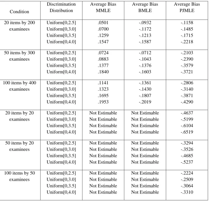
__4.4 Comparison of the average bias obtained by MML, BML, and PJML………..….42

__4.5 Results of PJMLE across the different simulation condition………...……..…….50

_ 4.6 Illustration of the effect of shrinkage methods on discrimination parameters……..…..50

__4.7 Concluding Remarks on Simulations ………..……...56

Chapter V..………..……….57

DISCUSSION………..………57

__5.1 Application of findings………...……….57

__5.2 Limitations of the findings ………….………...………..58

__5.3 Recommendations for Future Research ………...……59

REFERENECES………i_………60

i ii

LIST OF TABLES

Table Page

Table 1………. 30

Method of simulating item parameters and abilities along with a justification………. 30

Table 2………. 31

Formulas for estimating average RMSE, average bias and average absolute bias for item parameters and ability parameters ………. 31

Table 3………. 38

Illustration of the comparison of discrimination parameters from the fraction subtraction….... data set using both the MMLE method, BMLE method, and the PJMLE method ………..….. 38

Table 4………. 40

Comparison of the average RMSE of discriminations obtained by the three procedures ……. 40

Table 5………. 41

Comparison of the average RMSE of difficulties obtained by the three procedures …………. 41

Table 6………. 42

Comparison of the average RMSE of abilities obtained by the three procedures ………. 42

Table 7………. 43

Comparison of the average bias of discriminations obtained by the three procedures ………. 43

Table 8………. 44

Comparison of the average bias of difficulties obtained by the three procedures ………. 44

Table 9………. 45

Comparison of the average bias of abilities obtained by the three procedures ………. 45

Table 10………..…. 46

Comparison of the average absolute bias of discriminations obtained by the three procedures. 46 Table 11….……….……. 47

Comparison of the average absolute bias of difficulties obtained by the three procedures ….. 47

Table 12………..………. 48

Comparison of the average absolute bias iof abilities obtained by the three procedures ……... 48

i iii

LIST OF FIGURES

Figures Page

Figure 1………..…………. 9

Item response functions under the one parameter logistic model ………....…. 9

Figure 2………. 10

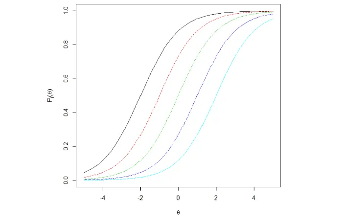
Item response functions under the two parameter logistic model……….……… 10

Figure 3………. 12

Item response functions under the three parameter logistic model.……….. 12

Figure 4……….………...………. 22

Example of a cross-validation plot obtained from the R help file ……….…. 22

Figure 5………. 27

Data structure of the first stage in the penalized joint maximum likelihood procedure. The responses are regressed on the starting ability estimates with an L1 penalty.………...…….…. 27

Figure 6……….……….…. 27

Data structure of the second stage in the penalized joint maximum likelihood procedure. The responses are regressed on the estimated discriminations with an L2 penalty.………..………. 27

Figure 7………. 51

Lognormal prior distribution used in the BMLE procedure ………..……. 51

Figure 8…...……….……. 52

Laplace prior distribution used in the PJMLE procedure ………..………. 52

Figure 9………. 53

Boxplots of the difference between MMLE estimate and true discrimination value One boxplot for each simulated value of the discrimination parameters.………..………. 53

Figure 10……….………. 54

Boxplots of the difference between BMLE estimate and true discrimination value One boxplot for each simulated value of the discrimination parameters.………..………. 54

Figure 11….………. 55

Boxplots of the difference between PJMLE estimate iand true discrimination value One boxplot for each simulated value of the discrimination parameters.………..………. 55

i iv

ACKNOWLEDMENTS

This dissertation could not have been completed without the unwavering support of many people. First, I am most deeply indebted to my advisor and mentor, Professor Matthew Johnson. He was very supportive of me throughout this whole process, and was always willing to help me when I had a question. His support and guidance made this possible. I would also like to thank my dissertation committee members, Professor Lawarence DeCarlo, Professor Young-Sun Lee, Professor John Black, and Professor Todd Ogden. Their valuable comments and questions on my paper and at my dissertation defense helped me to better explain my research and in doing so, helped me improve my research skill set. I am also thankful for family, Steve Paolino, Lee Paolino, and Chris Paolino for their love and support. I would also like to thank all of my friends that I have made while attending Columbia University, it was a true pleasure getting to know all of you on personal level. Lastly, I would like toithank the Human Development office staff, Mrs. Diane Katanik, Ms. Laurie Behrman, and Ms. Stephanie Phillips.

i

This thesis is dedicated to my family who have been a constant source of inspiration

i

i

1

Chapter 1: Introduction

1.1 Background of Item Response Theory

Item response theory (IRT) models are a conventional tool for analyzing both small scale and large scale educational data sets, and they are also used for the development of high-stakes tests such as the Scholastic Aptitude Test (SAT) and the Graduate Record Exam (GRE). As the name suggests there is a heavy focus on the development of test construction at the item level, which differentiates it from classical test theory (Fan, 1998). They are a class of statistical models used for repeated responses to items which assume an ordinal outcome measure. These models are primarily employed in psychometrics, but due to their increasing popularity are now being used in other academic disciplines such as social sciences (e.g., Spergel and Curry, 2005) and public health ( e.g., Shea, Tennant, and Pallant, 2009).

The IRT models used in this study are related in structure and usage to logistic regression in two respects. Structurally speaking, both types of models have a monotonic increasing "S" shaped function that takes on real number domain values and are bounded

between a range of zero and one. They are also similar because they aim to model the probability of an event happening. IRT models in educational data analysis are used to model the probability of an examinee answering a test item correctly as a function of the latent ability of the examinee and characteristics of the individual test item. In addition statistical models have certain

assumptions that must be fulfilled in order for the results to be valid. The results may be questionable if these assumptions are not met. The same rules apply for IRT models. 1.2 Shortcomings in Estimating IRT Models and Linear Models

2

In order to properly estimate the item parameters of IRT models the data set needs to include many more examinees than items. This is similar to regression modeling where more observations than variables are needed for the analysis. In both circumstances when this

stipulation has not been met it may be impossible to accomplish the analysis or the analysis may render results that are impossible to interpret. In certain instances it may not be possible to obtain an adequate sample size to accomplish the analysis. For example, a small classroom of twenty examinees could in theory be given an assessment of fifty items. Under this scenario item parameters would be not be estimable because the IRT model is not identified. This study

investigated a method for estimating IRT models when traditional methods were not appropriate. 1.3 Application of Penalized Estimation Methods

Penalized estimation methods have become an invaluable resource in statistical modeling when certain model requirements have not been fulfilled. This is important because real world data sets do not always satisfy all assumptions of statistical models. For example, one

requirement in regression analysis is that the independent variables are not multicollinear. When this requirement has not been met certain statistical inferences become impossible to accomplish. Ridge regression or L2 penalization (Hoerl & Kennard, 1970) was first introduced as a way to

obtain regression coefficients and to make accurate predictions even though the independent variables may be linearly dependent. Another example where a data set can violate assumptions is when the data set has many more variables than observations. Tibshirani (1996) introduced LASSO regression or L1 penalization for scenarios when there are many more variables than

3

that are most influential. A more detailed description of L1 penalization and L2 penalization is

presented in Chapter 2.

1.4 Applying Penalization Techniques to IRT

The main focus of this study was to apply L1 and L2 penalization techniques to IRT models

in order to better estimate model parameters. Particular interest was in applying these techniques to situations where the number of items greatly outnumbered the examinees. As previously stated this is a limitation in traditional regression and IRT estimation methods where dimensionality assumptions impose restrictions. In the context of IRT, this study looked at parameter estimation when the number of items was far greater than the number of examinees, as well as scenarios when the number of examinees outnumbered the number of items.

Another purpose of the study was to investigate if using L1 and L2 penalization yielded

item parameters and ability estimates with smaller mean squared errors. Based on maximum likelihood parameter estimates of certain examinee response patterns can yield estimates that are very large (in some cases infinity). Over-inflating of parameter estimates causes problems when attempting to interpret parameters. We hypothesized that by imposing a penalized model it prevents this over-inflating of item parameter estimates and should in theory shrink the total mean squared error of these estimates. In addition, we hypothesized that this new penalization technique would yield estimates with higher bias measures compared to traditional estimation techniques.

1.5 Overview of the Dissertation

The dissertation proceeds with a review of literature discussing frequently used

4

the methodology for applying penalization techniques to IRT is developed. The methods chapter includes a description of how the data sets were simulated and an explanation of the marginal maximum likelihood estimation method, the Bayesian maximum likelihood estimation method, and the penalized joint maximum estimation method. Due to a lack of consensus regarding proper nomenclature for the Bayesian procedure it is called Bayesian maximum likelihood estimation in this dissertation. The algorithm for computing the penalized joint maximum likelihood is described along with the equations for computing the average RMSE, the average bias, and the average absolute bias of the simulations in each condition. The results chapter begins with a real world data example. The data used was the fraction subtraction data set from Tatsuoka (1984). Next the diagnostic information from the simulations of the study is presented in the results chapter. A summary of the results is displayed according to the research evaluation criteria. The results section concludes with a discussion about the findings of the study including which research hypotheses have been confirmed and which have not. The discussion section addresses limitations of the study and possible future work in the area of penalized IRT.

5

Chapter 2: Review of Literature 2.1 Assumptions of Item Response Theory

As in any other statistical model, IRT models carry their own set of assumptions that must be satisfied for the results to be valid. They involve more statistically sophisticated

computation and therefore have more stringent assumptions than Classical Test Theory. First is the unidimensionality assumption, which states that the item pool (all items on the assessment) must measure only one latent trait. Examples of this one latent ability are mathematical ability, reading comprehension, or science knowledge. Research indicates that IRT models are robust against minor to moderate violations of this assumption (Hulin, C. L., Drasgow, F., & Parsons, C. K. 1983). This is a nice luxury because empirical data does not always satisfy the assumptions of statistical models. The second assumption is local independence, which states that the

probability of a correct response from the examinee is based solely on the ability of the examinee and each individual item, and not the interrelationship between multiple items. The third

assumption that is made is monotonicity, which describes the functionality between an

examinee's ability and performance on each item of the assessment. It states that there exists a monotonic non-decreasing relationship between examinee ability and the probability of giving a correct on the item. In other words, as examinee ability increases so does the probability of providing a correct response.

Sometimes it is useful to obtain a graphical illustration of IRT functions. This is achieved through an item characteristic curve (ICC). The ICC shows the functional relationship between the actual probability of an examinee correctly answering the item, given the ability of the examinee and other parameters of the item. It can display IRT functions that are specified by

6

one, two, or three parameters. Through various types of approximations parameter estimates are calculated to give information of the test items.

2.2 Dichotomous Items and Data Matrix Structure.

Only IRT models that assume a dichotomous item response structure were investigated in this study. They are among the most heavily researched topics in all of IRT. A dichotomous item in educational assessment takes on a value of zero for an incorrect response and one for a correct response. Examples of these items are multiple choice or True and False questions, as long as there is one and only one correct answer. Assume an assessment consisting of J dichotomously scored items is given to a group of N examinees, so that an N by J response matrix of zeros and ones can be constructed. When data collection has been completed one can impose IRT models on this N by J matrix to gain information about the items, and build item response functions from these estimates.

2.3 Review of Dichotomous Item Response Theory Models

In an academic setting, IRT models look to model the probability of a student answering an item correctly based on the characteristics of the item and the underlying latent ability of the examinee. IRT models have slightly different structures from each other. The fundamental structure of the unidimensional models used in this study is the logistic function shown in Equation 1.

As mentioned previously, the function takes on a range of values between zero and one,

so it is mathematically valid to use in order to estimate probability values. It is also assumed that each examinee answers each of the items so that an N by J matrix of zeros and ones can be

7

formed. An entry of one (Yij = 1) indicates that the item was answered correctly and an entry of

zero (Yij = 0) indicates that it was answered incorrectly. The models discussed in this review of

literature are the one-parameter model, two-parameter model, and three-parameter model. Each is specified by the number of item parameters and they all assume an underlying examinee latent ability. A parameter with j in the subscript is a reference to an item parameter, the ability

parameter of examinee i will always be denoted by θi , and the response of individual i to item j

will be Yij .

The first model discussed is the one-parameter model suggested by Rasch (1960). It is specified by one item parameter (known as the difficulty and denoted βj), the latent ability of the

examinee θi and a scaling constant α (also known as the discrimination parameter). The

mathematical form is represented below in Equation 2.

Notice that it looks similar to the logistic regression function except α(θi - βj) is

substituted in for x. According to this model the probability of a correct response to any item depends on the signed difference on the latent continuum between ability estimate θi and the

difficulty estimate βj . Mathematically, when θi is greater than βj the examinee has a greater than

50% chance of answering the item correctly, and when θi is less than βj the examinee has a worse

than 50% chance of answering the item correctly. Therefore the item difficulty parameter βj can

be thought of as the location on the latent continuum where the examinee has exactly a 50% chance of answering the item correctly. Also the one-parameter logistic model has a scaling parameter α, this is known as the item discrimination constant. In the one-parameter model and

8

Rasch Model it is forced to be equal across all the test items, meaning that each item has equal ability to discriminate amongst examinees. There are a couple of ways to include it when modeling a data set. In the Rasch Model α is forced to be one, and it is not estimated along with the abilities and difficulties. Equation 3 shows how the Rasch Model is written in IRT literature.

( ) ( ) Pr( 1| , ) 1 i j i j ij j i e Y e            ₍₃₎

Equation 3 shows a one-parameter model that does set α to equal one a priori. It is not estimated along with the abilities and difficulties and can take on any real number.

Mathematically the models are exactly the same except in the one parameter model one additional parameter is being estimated, so the Rasch Model can be thought of as a more

restrictive model (de Ayala, 2009). Figure 1 below illustrates item response functions fit using a one parameter model. The graph shows IRF’s that all are parallel but have different difficulty location.

9

Figure 1. Item response functions under the one parameter logistic model

In many cases it is not reasonable to assume that all items discriminate equally well

between all examinees. For this reason, the two-parameter logistic model is a popular option because it allows for varying levels of item discrimination (Birnbaum, 1968). Equation 4 shows a two parameter model with varying discrimination parameters. The discrimination parameter is related to the steepness of the IRF slope, larger αj’s produce IRF’s with a steeper slope than do

smaller αj’s. In understanding, IRF’s with larger αj’s have a better ability to discriminate between

different students. Under the two-parameter logistic model, the probability of a correct response is dependent on two item parameters, the discrimination and the difficulty of the item. Notice in Figure 2 below the two parameter model produces IRF’s that are not parallel to each other.

10 ( ) ( ) Pr( 1| , , ) 1 j i j j i j ij j j i e Y e              (4)

Figure 2. Item response functions under the two parameter logistic model.

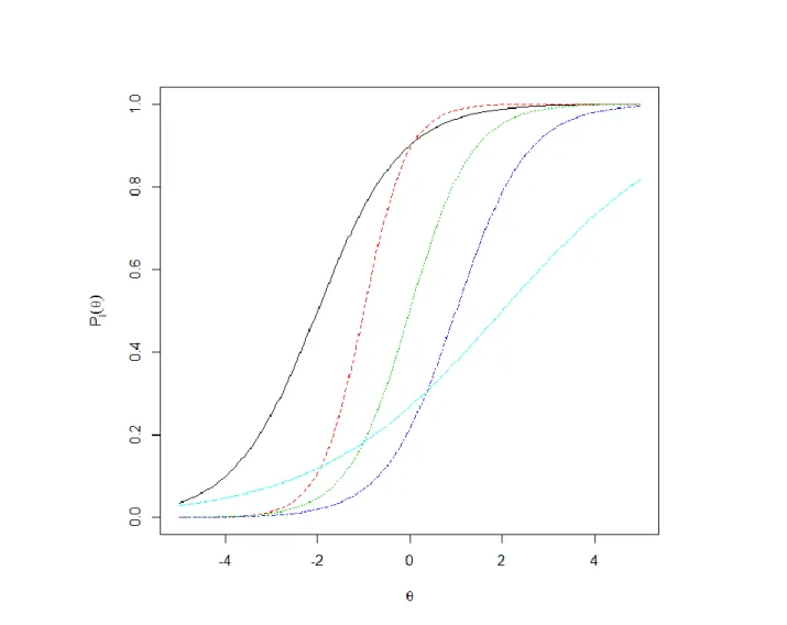
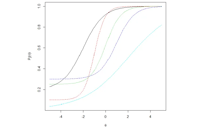
Finally, the last model is the three parameter logistic model (Lord, 1980). The three

parameter logistic model was developed to take into account the influence of guessing, which the Rasch Model and the two-parameter logistic do not. It does this by raising the lower asymptotic bound of the two-parameter logistic from zero to a new parameter ϛj . Equation 5 shows a three

parameter model with varying difficulty parameters, discrimination parameters, and guessing parameters.

11 ( ) ( ) Pr( 1| , , , ) (1 ) 1 j i j j i j ij j j j i j j e Y e                    ₍₅₎

The intuition behind this is that examinees with lower abilities have a higher probability

of obtaining a correct response because guessing is now being accounted for. A downside is that a larger sample of examinees is required to estimate all three item parameters (Foley, 2010). A classic example where the guessing parameter maybe very high is in the case of “True or False” items, if the examinees had no intellectual knowledge on how to answer the question guessing would give them a 50% chance of a correct response. However, on most standardized

assessments, there are usually four or five answer options to choose from, so the probability of a correct response just by guessing alone is a lot lower, closer to 25% and 20% respectively. Finally, an open ended item such as a “fill in the blank” item which the examinee has a lower chance of a correct response by guessing may have ϛj closer to but not exactly zero. Illustrations

12

Figure 3. Item response functions under the three parameter logistic model.

2.4 Estimating Parameters of Item Response Theory Models

As stated in Chapter 1, the main purpose of the study was to develop a new methodology for improving item parameter estimation when the number of items is much larger than the number of examinees. With this in mind, it is useful to review some of the most frequently used techniques in IRT parameter estimation. When analyzing dichotomous data the most widely used techniques are: Conditional Maximum Likelihood, Marginal Maximum Likelihood, Joint

Maximum Likelihood, and Bayesian Maximum Likelihood. Each method has its own special properties and limitations. There are other newer methods of parameter estimation such as

13

nonparametric estimation and multilevel estimation methods that are available to use under specific conditions.

The main idea behind IRT parameter estimation is the concept of maximizing different types of likelihood functions. In the context of IRT a likelihood function can be the probability of observing a particular pattern of responses from an individual, or it can be the probability of observing a particular response matrix. Since only dichotomous items are discussed only binomial likelihood functions are presented. Equation 6 represents the likelihood function of observing a particular response matrix.



The first type of estimation is conditional maximum likelihood (CML) Andersen (1970),

which is specific only to the Rasch model. CML aims to model the probabilities of a particular item response pattern conditional on the total score of the individuals test, also known as the raw score. In this case the total score Ti, where Ti = Yi1+Yi2+…+Yij, serves as a sufficient statistic for

θi.

Equation 7 displays the Conditional Likelihood Function that gets maximized with respect to the β’s to get item difficulty estimates. In CML the θ’s are treated as nuisance

parameters and therefore only estimates of the β’s are obtained (notice the conditional likelihood function does not depend on θ). This method has very useful statistical properties in that

14

parameter estimates are unbiased and consistent. However, due to the restrictive nature of The Rasch Model, CML is very seldom used.

The next type of estimation is called marginal maximum likelihood (MML). MML treats the N individuals as observational units and assumes that they are random effects sampled from a mixing distribution f(θ|v) (Johnson, 2007). The mixing distribution describes how θ is distributed in the population, and it is usually assumed to have a standard normal distribution. Together the IRT model and the mixing distribution allows for the calculation of the marginal probability of a particular response pattern. Below is how the marginal likelihood function is defined (de Ayala, 2009).

_





The marginal likelihood function (Equation 9) is now unconditional on θ because

Equation 8 integrates over all possible values of θ. The next step would be to maximize this likelihood function with respect to the item parameters to derive the MML estimates (Johnson, 2007). Equation 10 is an example of a marginal probability function of a two-parameter logistic model with a mixing distribution of θ~N(0,1). Suffice it to say that it is a very difficult problem to solve analytically and it must be approximated by numerical quadrature (Johnson, 2007).





15

The next type of parameter estimation is joint maximum likelihood (JML). Instead of treating the N individuals as the observational units as in MML, JML treats the N x J item responses as the observational units (Johnson, 2007). In addition, this method treats the item parameters and examinee abilities as fixed parameters and thus the procedure yields estimates for both. Essentially, the method of JML estimation is based on logistic regression with dummy variables for the item parameters and examinee abilities. The procedure begins with provisional estimates of examinee ability locations and these are treated as known for estimating the items’ parameters via Newtons method (de Ayala, 2009). Once convergence is obtained for the item parameter estimates, these estimated item parameters are treated as “known” and the person locations are re-estimated again via Newton’s method. This method goes back and forth until the difference between successive iterations is sufficiently small. The improved examinee ability estimates are treated as “known” and the item parameters are considered reestimated (de Ayala, 2009). The item parameter estimation techniques were based on the JML procedure. For

simplicity, I referred to this novel estimation technique as Penalized Joint Maximum Likelihood (PJML).

The last type of parameter estimation is Bayesian maximum likelihood (BML). In Bayesian maximum likelihood estimation a posterior distribution for each item parameter is calculated by multiplying the likelihood function by a prior distribution function. Once the posterior distribution has been obtained, a procedure known as Maximum A Posteriori (MAP) is used to find the mode of the posterior distribution, this measure serves as the Bayesian estimate for the item or person parameter. One could also use an estimation procedure called Expected A Posteriori (EAP), which computes the expected value of the posterior distribution. However, it is more computationally intense so it is not as popular. Equation 11 illustrates a formula to compute

16

a posterior distribution function which is obtained by the product of the likelihood function and the prior distribution on the discriminations.

f( , , |   X) f X( | , , )   f( ) (11)

2.5 Background Literature In Small Sample IRT

Although no novel parameter estimation techniques have been developed so far when the number of items outnumbers the number of examinees, significant progress has been made in IRT when the sample of examinees and/or items is “small.” Many small sample methods involve applying Bayesian estimation methods. The main idea of this method is to include prior

information about item parameters to the likelihood functions. This prior information is also known as a prior distribution function. Swaminathan and Gifford (1982, 1985, 1986) provide extensive empirical evidence that when the number of examinees and/or items is small, Bayesian estimates correlate higher with true values than do traditional maximum likelihood estimates. These results hold true for the one-parameter model, two-parameter model, and three-parameter model. The efficacy of Bayesian methods is further evidenced by Setiadi (1997) where it was concluded that not only were Bayesian estimation methods comparable to regular likelihood methods, they consistently outperformed standard nonparametric estimation procedures. Foley (2010) investigated Bayesian parameter estimation using a data augmentation technique called the “DupER.” This method generates additional plausible response vectors based on observed response patterns from the original data. Additional responses and original responses were combined to fit a three-parameter model then parameter diagnostics were analyzed. The results of the analysis were mixed and inconclusive. The data augmentation

17

algorithm tended to result in larger root mean squared errors and lower correlations between estimates and parameters for both item and ability parameters.

Cho and Rabe-Hesketh (2012) proposed a method of shrinking item discrimination parameters towards the mean of the overall discrimination parameters (indicated by γ in Equation 12). Their method of random item discrimination marginal maximum likelihood estimation is achieved through an algorithm called alternating imputation posterior (AIP). Recall in marginal maximum likelihood, it is assumed that the θi come from a mixing distribution

N(0,1), and the marginal maximum likelihood function is obtained by integrating over all

possible values of θi. The integrating over all possible values of θi allows the resulting likelihood

function to become unimodal, which is then approximated by numerical quadrature.

They proposed treating the discriminations as a latent random variable that gets integrated out along with the abilities. It starts by assuming that the abilities come from a standard normal distribution and the discriminations come from the distribution :

αi = γ + ai (12)

In Equation 12, the discriminations are denoted by ai which come from a N(0, ψ). The

goal is to estimate γ, ψ, and ai simultaneously with βj and θi . As the name suggests there is an

alternating between two stages until convergence has been achieved. Cho and Rabe-Hesketh (2012) thoroughly explain the algorithm. They showed using real data and simulations, that AIP yields more stable and accurate discrimination parameter estimates than marginal maximum likelihood estimation, marginal Bayes modal estimation, and Markov chain Monte Carlo estimation.

18 2.6Overview of Penalized Regression Techniques

L1 penalization or LASSO (Tibshirani, 1996) is a type of regression technique that places

a penalty on the absolute value of the regression coefficients. This approach shrinks the overall vector of regression parameter estimates, and sets a number of them equal to zero yielding a “sparse” solution. This in effect is a form of continuous variable selection, with the zeroed coefficients being removed from the model. The main attraction of LASSO and other penalization techniques is that solutions exist when the number of variables outnumbers the sample size (p>n). When p>n traditional regression methods can not be utilized because of dimensionality restrictions. In the context of linear regression, the LASSO procedure seeks to minimize the function:

2 0 1 1 1 ( ( )) | | p p n Lasso i j ij j i j j Q_ Y   X      







No closed form solution to L1 penalization exists because the objective function is not

differentiable (Tibshirani, 1996). However, quadratic programming procedures can be applied to arrive at a solution. Also note there is a tuning parameter λ which determines how much

shrinkage is applied. Choosing the tuning parameter λ will be discussed later on. In terms of Bayesian estimation, LASSO can be thought of as putting a Laplace prior on the standardized regression coefficients with normal likelihood function.

2 0 1 1 1 ( ( )) | | p p n i j ij j i j j Y X Lasso Posterior Q e e              (14)

L2 penalization or ridge regression (Hoerl & Kennard,1970), is a technique that places a

19

vector of regression parameter estimates, but does not yield a sparse solution. For the n>p case ridge regression outperforms the LASSO in terms of predictive performance when there is high correlation among the independent variables. However, the set of parameter estimates in ridge regression is very difficult to interpret, so usually LASSO is the more sensible option. In the context of linear regression, the ridge regression procedure seeks to minimize the function:

2 2 0 1 1 1 ( ( )) p p n Ridge i j ij j i j j Q_ Y   X      







One redeeming quality of L2 penalization is that a closed form solution does exist, because

no absolute values are included. Again the tuning parameter λ determines how much shrinkage is applied. In terms of Bayesian estimation, ridge regression can be thought of as putting a normal prior on the standardized regression coefficients with normal likelihood function.

2 2 0 1 1 1 ( ( )) p p n i j ij j i j j Y X Ridge Posterior Q e e              (16)

The last type of penalization technique is called elastic net estimation (Zou & Hastie, 2005). Elastic net is a compromise between L1 and L2 penalization, the distinguishing feature is

how it deals with groups of variables that are correlated. Groups of highly correlated variables are either entirely left of the model or entirely left in (Zou & Hastie, 2005). LASSO will tend to discard part of the group, making interpretation difficult. In addition, elastic net gets potentially allows all the predictors to be included in the model. The elastic net procedure seeks to minimize the function:

20 1 2 . 2 2 , 0 1 2 1 1 1 1 ( ( )) | | p p p n E Net i j ij j j i j j j Q  Y   X         









Notice the penalized models are examples given in the context of least squares regression. Penalization techniques can be conveniently applied to many generalized linear models. For example, in logistic regression function adding an L1-penalty to the binomial

likelihood functions gives the following equation:

QLasso = _{0 0} 1 1 1 1 arg min ( ( )) [1 exp( )] | | p p p N N i j ij e j ij j i i j i j j y   x Log   x             











2.7 Choosing Tuning Parameters

The ultimate goal of statistical modeling is to produce a model that can predict well. Traditional linear and logistic regression methods have the advantage of producing parameter estimates with good statistical properties (unbiasedness and consistency). However, research has shown that imposing an unbiased model on the data does not always produce estimates with optimal prediction potential as measured by mean squared error (linear regression) or binomial deviance (logistic regression). The process of finding a model with the lowest MSE or binomial deviance is known as variance-bias tradeoff. The amount of bias to include as indicated by λ can be found through AIC, BIC, or k-fold cross validation. The problem with using AIC and BIC is that both are not defined for p>n, so they are rarely used for penalization purposes. Therefore, cross-validation is most often the favorable choice for choosing λ and it was the only method used in the study.

Different values of the penalty λ lead to different parameter estimates (Johnson, 2011). One approach to selecting a penalty term is to try a sequence of λ values and then select the λ value that leads to the smallest prediction error (Tibshirani, 2001). K-fold cross validation (which is

21

one way to measure prediction error) splits the data into k non-overlapping

partitions(T1,T2,…Tk), which is then broken down into k-1 partitions used for training and one

partition used for testing. The penalized regression model with a particular value for λ is then imposed on each of the k-1 training partitions then finally on the testing partition. Within each partition estimated values are computed from the data for a particular λ then they are subtracted from the actual response values, and finally squared. The next step is to divide the sum squared error by the sample size of each partition nk to get an average mean squared error for the kth fold.

This is then averaged again over the k partitions and for a particular λ value. The model would then have an overall cross validation error expressed by the following Equation 19 (Tibshirani, 2001). ( ) / ( ) 2 0 1 1 ( ) ( ( )) / k k m m i i k m i T MSE y x n k      



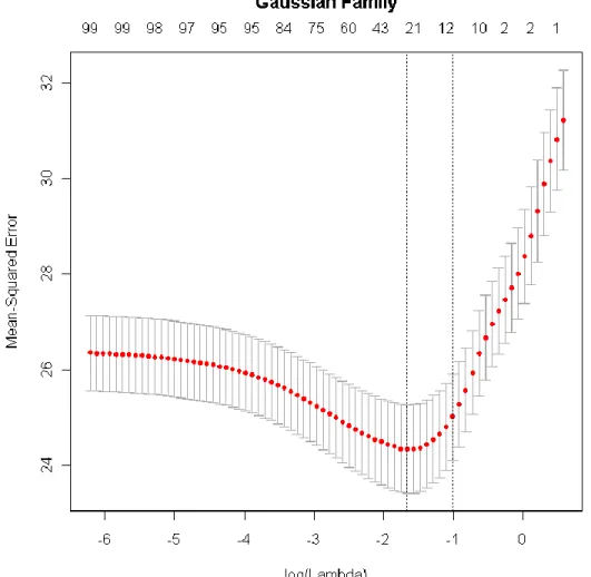
One should choose the λ value that minimizes the above function. Typically, this is illustrated by a cross-validation plot where different values of λ are shown on the horizontal axis and the prediction error rate (MSE or deviance) is displayed on the vertical axis. Statistical packages now include user friendly methods for obtaining cross validation plots. Once a satisfactory λ is chosen, one may refit the entire data based on the chosen λ and compare the errors rates of the penalized model compared to the full non-penalized model simply for

comparison. Unfortunately, no reference distributions exist for penalized models so there can be no formal model comparison. Figure 4 is example of a cross-validation plot which was obtained from the R help file. The numbers at the top of the plot indicate how many variables will be left in the model. The vertical axis indicates the mean-squared error and the horizontal axis indicates the logarithm of the different λ values.

22

____________________________________________________________________________________

Figure 4. Example of a cross-validation plot obtained from the R help file

As far as choosing λ1 and λ2 for elastic net penalization is concerned it is done in a similar

way. However, instead of using a two dimensional plot with a cross-validation curve, a three dimensional plot (λ1 on one axis, λ2 on another axis, and prediction error on the vertical axis)

with a cross-validation region is used (Zou & Hastie, 2005). Again, with help of statistical packages λ1 and λ2 can be easily obtained.

23

Penalized estimation methods are a relatively new topic in statistical modeling. That said the best available program to fit penalized models is R using the “glmnet” package (Friedman et al., 2010). This package computes solutions to all penalized generalized linear models using a fast algorithm known as cyclical coordinate descent and it was used for this study. SAS has a procedure called GLMSELECT that fits penalized models which is currently in the development, but despite the name it only computes solutions to linear regression models.

24

Chapter 3: Methods

3.1 Introduction

The IRT model that was used for this study was the two-parameter logistic model. Particular attention was given to the item discrimination parameters, which is the distinguishing feature of the model, however, the difficulty parameters and ability estimates were also analyzed. As described in the previous chapters the main purpose of this study was to investigate a new estimation procedure for analyzing a dichotomous IRT data set when the number of items outnumbers the number of examinees. However, for the sake of completeness the estimation diagnostics of all conceivable item and examinee structures were analyzed. In other words, we looked at different combinations of number of examinees and number of items and then compared the estimation techniques of traditional IRT parameter estimation methods to this novel estimation method. In this study the marginal maximum likelihood parameter estimation (MMLE) procedure and Bayesian maximum likelihood estimation procedure (BMLE) were compared to the method of penalized joint maximum likelihood estimation (PJMLE). Part of the evaluation criteria in the study was to indicate which parameter estimation methods are most appropriate to use under each matrix dimension structure. In addition, the root mean squared errors (RMSE) and the bias of the discriminations parameters, difficulty parameters, and the examinee ability parameters were computed for the three different methods. The computational formula for RMSE and bias will be discussed later on in the chapter. The statistical program R (R Core Development Team, 2011) was used to accomplish the analysis. The packages within the R program that were used were glmnet (Friedman et al., 2010), ltm (Rizopolous, 2006), and irtoys (Partchev, 2012).

25

3.2 IRT Estimation using Penalized Joint Maximum Likelihood and GLMNET

Recall, the method of traditional JML estimation is based on logistic regression with dummy variables for the item parameters and examinee abilities. Parameter estimates are obtained when the iterative convergence algorithm yields differences between successive examinee ability estimates that are sufficiently small.

The R package that was used to run the LASSO and the ridge procedure in the penalized joint maximum likelihood procedure was glmnet. Penalized joint maximum likelihood is a two stage estimation procedure that is based on the same principles of traditional JML. After the response matrix has been simulated the N x J item responses are put into an NJ x 1 vector form then regressed on the starting values of the θ's with an L1 penalty shown in Equation 20 using the

glmnet package. This allows for obtaining the L1-α's which are the logistic regression parameters.

The λ tuning parameter which determines how much shrinkage is applied during estimation is obtained by k-fold cross validation. In glmnet there is an option for how many folds (with a minimum of 3) that the user must specify. We chose to use 10-fold cross validation. This method divides the data set into ten equal parts and performs logistic regression with L1 penalization on

each of the ten divided data sets for a given λ then the overall average error rate is computed over the ten folds. Glmnet repeats this process using a sequence of different λ values and then the regression coefficients with the λ value that gives the lowest error rate is selected for the model. Then these regression parameter values are extracted by a simple command and are then used in the second stage. The data structure for this first stage is illustrated below as Figure 5. The penalized likelihood function that gets optimized in stage one is:





26

In the second stage, the NJ x 1 vector of item responses are regressed on the estimated item parameter estimates with the regression coefficients from stage 1 serving as estimates for the discriminations. The goal in this stage is to use an L2 penalty to obtain the re-estimated L2-θ’s.

This is again done through L2-penalized logistic regression using the glmnet package. Once again

10-fold cross validation is used in the exact same way as stage 1 to obtain the regression coefficients. These re-estimated L2-penalized regression coefficients are extracted by a simple

command and then are placed back into stage one and the algorithm cycles through again. The data structure for this second stage is illustrated below as Figure 6. The penalized likelihood function that gets optimized in stage two is by Equation 21.





This method goes back and forth between the two stages until the difference between successive re-estimated L2-θ’s is sufficiently small (10-6). Once the algorithm has converged the final

parameter estimates are referred to as the L1-α's, L2-β’s and the L2-θ’s. The intuition behind

putting an L1 penalty on the α's was to zero-out discriminations that are small while leaving

others in with some shrinkage. This also may allow researchers to flag items that do not discriminate well. The reasoning for putting an L2 penalty on the β’s and θ’s was so the

27 11 1 21 2 1 12 1 22 2 2 1 1 2 2 0 . . . 0 0 . . . 0 . . . . . . . . 0 . . . 0 0 0 . . . 0 0 0 . . . 0 . . . . . . . . 0 0 . . . 0 . . 0 . . . . . . . . 0 . . . 0 0 . . . 0 . . . . . . . . N N N N J J Y Y Y Y Y Y Y Y         0 0 . . . 0 NJ N Y  _____________________________________________________________________________________

Figure 5. Data structure of the first stage in the penalized joint maximum likelihood procedure. The

responses are regressed on the starting ability estimates with an L1 penalty.

11 1 21 1 1 1 12 2 22 2 2 2 1 2 0 . . 0 1 0 . . 0 0 0 . . 1 0 . . 0 . . 0 . . . . . . . . 0 0 . . 1 0 . . 0 0 . . 0 0 1 0 . 0 0 0 . . 0 1 0 . 0 . . 0 . . . . . . . . 0 0 0 . 0 1 0 . 0 . . . 0 . . . . . . . . . 0 . . . 0 1 0 0 . . . 0 1 . . 0 . . . . . . . . N N J J J J Y Y Y Y Y Y Y Y         0 0 . . 0 . . 0 1 NJ J Y  ________________________________________________________________________

Figure6. Data structure of the second stage in the penalized joint maximum likelihood procedure. The

28

according to a two parameter model using the simulated item parameters and ability values and then the responses are put into a vector form. A function is then created. In the beginning of the function, the first glmnet procedure uses the vector of item responses which serves as the

dependent variable and the design matrix of ability estimates which are shown in Figure 5 serves as the independent variables. Then the glmnet procedure with an L1-penalty is applied. The

regression coefficients from the first procedure serve as the estimated discriminations for the second glmnet procedure. The second glmnet procedure uses the response vector once again as the dependent variable and the design matrix is a combination of two matrices as shown in Figure 6 which serves as the independent variables. Then the glmnet procedure with an L2

-penalty is applied. The regression coefficients obtained from the input of discriminations serves as the reestimated ability estimates and this completes one loop of the function. Using these reestimated ability estimates the function loops back to start at the beginning and the process begins all over again. The function iterates back and forth between the glmnet L1-penalty

procedure and the glmnet L2-penalty procedure until successive iterations produce reestimated

abilities that are negligibly small, less than 10-6. 3.3 IRT Estimation using ltm

The ltm package (Rizopolous, 2006) was used for estimating the two-parameter logistic model by marginal maximum likelihood. It took only one command to obtain the item

parameters estimates and took an additional command to obtain the true ability estimates. In order to calculate the root mean squared error and bias measures the estimated values needed to be exported from the ltm output. After the measures were exported the RMSE and bias measures were computed using a second step procedure R.

29 3.4 IRT Estimation using irtoys

The Bayesian estimation procedure was accomplished using the irtoys (Partchev, 2012) and ICL (Hanson, 2002) packages. The irtoys package used the algorithm from the ltm package to obtain the marginal likelihood function and in conjunction put a prior distribution on the item parameters. The prior distribution for the discrimination parameters was a lognormal distribution with mean equal to zero and standard deviation equal to ½, also noted as lnN(0, .5). The prior distribution for the difficulty parameters was a normal distribution with mean equal to zero and a standard deviation of two, also noted as N(0, 2). Once the procedure finished, it took one

command to obtain the discrimination estimates and difficulty estimates then an additional command to obtain the ability estimates. RMSE and bias measures were calculated after the estimates had been obtained.

3.5 Evaluating RMSE and Bias through simulation

In statistical research it is critical to show that results hold up after repeated trials. For this reason, one-thousand simulated data sets for each response structure (Examinees by Items) were generated by starting values for examinee abilities and item parameters. There were two hundred and fifty replications of data sets from each of four different uniform discrimination distributions for each experimental condition. The four uniform distributions that we used were U[0, 2.5], U[0, 3.0], U[0, 3.5], and U[0, 4.0]. We used uniform distributions all with a lower bound of zero to ensure that every possible true discrimination value could be included in the study. We also wanted to see how the procedure estimated discriminations that were close to zero. In addition, the uniform distributions we chose ensured a fair sampling of high and low discriminating items. There were six different experimental matrix structures. Just to

30

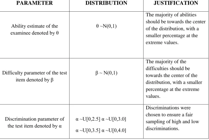
summarize, each of the six different conditions had one thousand simulated data sets for a total of six thousand data sets. Table 1 below describes how the parameters will be simulated along with justification.

PARAMETER DISTRIBUTION JUSTIFICATION

Ability estimate of the examinee denoted by θ

θ ~N(0,1)

The majority of abilities should be towards the center of the distribution, with a smaller percentage at the extreme values.

Difficulty parameter of the test item denoted by β

β ~ N(0,1)

The majority of the difficulties should be towards the center of the distribution, with a smaller percentage at the extreme values.

Discrimination parameter of the test item denoted by α

α ~U[0,2.5] α ~U[0,3.0] α ~U[0,3.5] α ~U[0,4.0]

Discriminations were chosen to ensure a fair sampling of high and low discriminations.

________________________________________________________________________

Table 1. Method of simulating item parameters and abilities along with a justification

Each time a data set was simulated the MMLE, BMLE, and the PJMLE procedures were used to obtain parameter estimates. Then the RMSE, bias, and absolute bias measures for the discrimination estimates, difficulty estimates, and examinee abilities were computed by a second step procedure. RMSE is a measure of precision of the parameter estimates. Smaller values for RMSE are preferred because they are an indication that the true values do not deviate much from

31

the estimated values for a particular estimation method. RMSE is a very important measure however, it does not indicate if the parameter estimates are consistently too high or too low. Another measure that we looked at was bias. Estimation procedures with lower average bias for discriminations, difficulties, and abilities are preferred because it is an indication that the estimates do not deviate as much from the true values. There are two methods for computing bias. One way is to take the absolute value of the difference from the true value and the estimated value. The reason this is done is to protect against the negative and positive values canceling each other out and thus misrepresenting the actual difference between the true value and the estimates. It is also possible to compute the bias without taking an absolute value. This gives insight into whether the estimation procedure underestimates or overestimates the true value of the parameter. Table 2 shows the formulas were used to compute average RMSE, average bias, and average absolute bias.

Formula Description of Formula

_________ 2 1 1 1 1 _ˆ ( ) ( ) J R jr j j r RMSE J R     



 

_________ 2 1 1 1 1 _ˆ ( ) ( ) J R jr j j r RMSE J R     



 

_________ 2 1 1 1 1 _ˆ ( ) ( ) N R nr n n r RMSE N R     

32 ______ 1 1 1 1 _ˆ ( ) ( ) J R jr j j r Bias J R     



 

______ 1 1 1 1 _ˆ ( ) ( ) J R jr j j r Bias J R     



 

______ 1 1 1 1 _ˆ ( ) ( ) N R nr n n r Bias N R     



 

___________ 1 1 1 1 _ˆ ( ) | | J R jr j j r Absbias J R     



 

___________ 1 1 1 1 _ˆ ( ) | | J R jr j j r Absbias J R     



 

___________ 1 1 1 1 _ˆ ( ) | | N R nr n n r Absbias N R     



 

Table2. Formulas for estimating average RMSE, average bias and average absolute bias for item

parameters and ability parameters.

3.6 Description of Different Matrix Dimensions

Item response data sets have the capability of taking on many different item by examinee structures depending on factors such as the number of examinees desiring to partake in the assessment and the number of items educators deem appropriate. Some matrices may have more items than examinees and others may have more examinees than items. Nowadays, academic assessments can range in length anywhere from a few items to several hundred items. Therefore, it is imperative to simulate IRT data matrices that resemble these scenarios. We simulated one thousand of each of the following matrix structures:

33 1. 20 items and 200 examinees

2. 50 items and 300 examinees 3. 100 items and 400 examinees 4. 20 items and 20 examinees 5. 50 items and 20 examinees 6. 100 items and 50 examinees 3.7 Research Questions and Hypotheses

The research questions that this study looked to answer are as follows:

1. Can penalized joint maximum likelihood be used to estimate item parameters of a two-parameter logistic model as well as examinee ability estimates when it is dimensionally inappropriate to use marginal maximum likelihood and Bayesian maximum likelihood?

2. How does the root mean squared error of examinee abilities and item parameters compare under penalized joint maximum likelihood, marginal maximum likelihood, and Bayesian maximum likelihood?

3. How does the bias and absolute bias of examinee abilities and item parameters compare under penalized joint maximum likelihood, marginal maximum likelihood and Bayesian maximum likelihood?

We hypothesized that using penalized joint maximum likelihood would allow for

estimating item parameters and examinee abilities even when it is dimensionally inappropriate to use marginal maximum likelihood and Bayesian maximum likelihood which are traditional techniques. Also, we hypothesized that penalized joint maximum likelihood would produce item parameters and examinee abilities with a smaller root mean square error than marginal maximum likelihood and Bayesian maximum likelihood. Finally we hypothesize that penalized joint

34

maximum likelihood would produce item parameters and examinee abilities with a larger bias and absolute bias than marginal maximum likelihood and Bayesian maximum likelihood.

35

Chapter 4: Results 4.1 Overview of the findings

The paramount finding was that PJMLE provided estimates to item and ability parameters when it was dimensionally inappropriate (more items than examinees) to use MMLE and BMLE when estimating a two parameter IRT model. Also, in many of the experimental conditions of the simulation study PJMLE yielded parameter estimates with lower average RMSE but more average bias and average absolute bias than MMLE. However, BMLE significantly

outperformed PJMLE and MMLE when the dataset included more examinees than items, mainly because the priors that were used were highly informative. It is also important to note that the tuning parameter associated with LASSO and Ridge estimation focuses on optimizing prediction not necessarily on optimizing bias. This may explain why BMLE outperformed PJMLE.

4.2 Applying MMLE, BMLE, and PJMLE to a real data set.

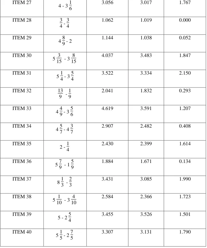
The real data set that we used is the well known fraction subtraction data set from Tatsuoka (1984). This data set is from an exam consisting of forty dichotomously scored items taken by five-hundred and thirty-six examinees. The data was analyzed using marginal maximum likelihood estimation, Bayesian maximum likelihood estimation and penalized joint maximum likelihood estimation. Table 3 displays a comparison of the discrimination parameters obtained by MMLE, BMLE and PJMLE. Notice that the PJMLE produced discrimination parameters that are all smaller than MMLE and BMLE with some being shrunk to zero. An interesting finding was that the PJMLE procedure shrunk the discrimination parameters to zero for items that did not necessarily measure fraction subtraction skills, for example Item 8 and Item 28. However we believe more research is needed to confirm these assertions. Unfortunately, no IRT data set is

36

known to have a structure where the number of items is greater than the number of examinees. However, makeshift methods for obtaining an IRT data having more items than examinees can be used. For example, one could partition the Fraction Subtraction data set into smaller parts to create a data set that has forty items and a random sample of twenty response patterns.

ITEM NUMBER ACTUAL ITEM MMLE -

α

α

ITEM 1 5 3 - 3 4 2.213 2.015 1.392 ITEM 2 3 4 - 3 8 2.847 2.615 1.641 ITEM 3 5 6 - 1 9 2.386 2.212 1.521 ITEM 4 3 1 2 - 2 3 2 1.422 1.336 1.040 ITEM 5 4 3 5 - 3 4 10 1.088 1.015 0.171 ITEM 6 6 7 - 4 7 2.488 2.250 0.000 ITEM 7 3 - 2 1 5 2.426 2.341 1.493 ITEM 8 2 3 - 2 3 1.107 1.051 0.000 ITEM 9 3 7 8 - 2 0.834 0.773 0.000 ITEM 10 4 1 3 - 2 4 3 3.014 2.633 1.618 ITEM 11 4 1 3 - 2 4 3 2.681 2.471 1.879

37 ITEM 12 11 8 - 1 8 2.142 1.920 0.059 ITEM 13 3 3 8 - 2 5 6 2.912 2.709 1.125 ITEM 14 3 4 5 - 3 2 5 2.594 2.309 0.298 ITEM 15 2 - 1 3 2.650 2.564 1.783 ITEM 16 4 5 7 - 1 4 7 2.195 1.925 0.280 ITEM 17 7 3 5 - 4 5 2.982 2.777 1.881 ITEM 18 4 1 10 -2 8 10 2.221 2.103 1.506 ITEM 19 4 - 1 4 3 3.435 3.524 1.404 ITEM 20 4 1 3 - 1 5 3 3.112 2.881 1.796 ITEM 21 8 5 - 5 6 2.634 2.403 1.631 ITEM 22 5 3 - 5 6 3.116 2.832 1.809 ITEM 23 5 6 - 1 15 3.334 2.978 1.934 ITEM 24 4 1 3 - 3 4 3 1.057 1.013 0.629 ITEM 25 3 2 3 - 2 2 6 2.401 2.133 1.444 ITEM 26 3 4 - 2 4 3.488 2.881 0.000

38 ITEM 27 4 - 3 1 6 3.056 3.017 1.767 ITEM 28 3 4 - 3 4 1.062 1.019 0.000 ITEM 29 4 8 9 - 2 1.144 1.038 0.052 ITEM 30 5 3 15 - 3 8 15 4.037 3.483 1.847 ITEM 31 5 1 4 - 3 5 4 3.522 3.334 2.150 ITEM 32 13 9 - 1 9 2.041 1.832 0.293 ITEM 33 4 4 9 - 3 5 6 4.619 3.591 1.207 ITEM 34 4 5 7 - 4 3 7 2.907 2.482 0.408 ITEM 35 2 - 1 4 2.430 2.399 1.614 ITEM 36 5 7 9 - 1 5 9 1.884 1.671 0.134 ITEM 37 8 1 3 - 2 3 3.431 3.085 1.990 ITEM 38 5 1 10 - 3 4 10 2.584 2.366 1.723 ITEM 39 5 - 2 5 4 3.455 3.526 1.501 ITEM 40 5 1 5 - 2 7 5 3.307 3.131 1.790 ____________________________________________________________________________________

Table 3. Illustration of the comparison of discrimination parameters from the fraction subtraction data set

39

4.3 Comparison of the average RMSE obtained by MMLE, BMLE, and PJMLE Estimation procedures with lower average RMSE for discriminations, difficulties, and abilities are preferred because it is an indication that the estimates do not deviate as much from the true values. RMSE is more a measure of variability of the point estimates. Accuracy of the point estimates is better measured by bias, which will be discussed in the next section. PJMLE was successful in providing estimates of RMSE when the number of items was far greater than the number of examinees. BMLE and MMLE failed to provide meaningful results of RMSE when the number of items outnumbered examinees.

Table 4 displays a comparison of the average RMSE of discriminations obtained by the three estimation procedures in the six different conditions. In each of the comparable conditions BMLE provided the smallest measure of RMSE compared to MMLE and PJMLE for the discrimination parameters. PJMLE gave better estimates of the RMSE of the discriminations compared to MMLE in the 100 item by 400 examinee condition. Mixed results were given in both the 20 item by 200 examinees condition and the 50 item by 300 examinee condition. Table 5 represents the RMSE of the difficulties produced by the three estimation methods. BMLE clearly outperformed both MMLE and PJMLE producing lower RMSE in all of the experimental conditions. It was inconclusive as to which estimation procedure was more accurate MMLE or PJMLE. Although, MMLE seemed to perform better than PJMLE in the 20 item by 200 examinees condition. In addition, PJMLE was able to yield estimates of difficulties even when the number of items was larger than the number of examinees.

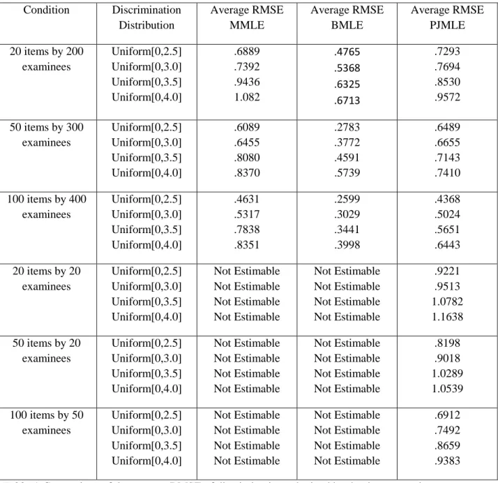
Table 6 displays a comparison of the average RMSE of abilities obtained by the three