A Probabilistic Hypothesis Density Filter for Traffic
Flow Estimation in the Presence of Clutter
Matthieu Canaud
∗, Lyudmila Mihaylova
†, Nour-Eddin El Faouzi
∗‡, Romain Billot
∗‡and Jacques Sau
∗ ∗Universit´e de Lyon, F-69000, Lyon, FranceIFSTTAR, LICIT, F-69500, Bron ENTPE, LICIT, F-69518, Vaulx en Velin
Email: [email protected] †School of Computing and Communications InfoLab21, South Drive, Lancaster University
Lancaster LA1 4WA, UK Email: [email protected]
‡Smart Transport Research Centre Faculty of Build Environment and Engineering,
Queensland University of Technology
2 George St GPO Box 2434, Brisbane QLD 4001, Australia
Abstract—Prediction of traffic flow variables such as traffic volume, travel speed or travel time for a short time horizon is of paramount importance in traffic control. Hence, the data assimilation process in traffic modeling for estimation and pre-diction plays a key role. However, the increasing complexity, non-linearity and presence of various uncertainties (both in the measured data and models) are important factors affecting the traffic state prediction. To overcome this problem, new methodologies have been proposed. With this aim, in this paper we propose the use of the Probability Hypothesis Density (PHD) filter for traffic estimation. This methology is intensively studied, developed and improved for the purposes of multiple object tracking and consists in the recursive state estimation of several targets by using the information coming from an observation process. However, some issues need to be studied, especially the impact of the clutter (false alarm) intensity. The goal of this paper is to expose the potential of the PHD filters for real-time traffic state estimation and the choice of an appropriate clutter intensity. This investigation is based on a Cell Transmission Model (CTM) coupled with the PHD filter. It brings a novel tool to the state estimation problem and allows one to estimate the densities in traffic networks. In this work, we compare this PHD filter with the particle filter (PF) which has been successfully applied in traffic control and conclude that the PHD filter can be seen as a relevant alternative that opens new research avenues.
I. INTRODUCTION
Advanced estimation methods and sensor data fusion can improve the traffic conditions in Intelligent Transportation Systems (ITS) and provide information about special events. The fact that the full benefits of these systems cannot be realized without an ability to predict short-term traffic condi-tions has been emphasized by Sussman [20]. Hence, short-term prediction of traffic states appears as a key point in various ITS applications such as Advanced Traffic Management Systems (ATMS). In this context, prediction of traffic flow variables such as traffic volume, travel speed or travel time for a short time horizon (typically 5 up to 30 minutes) is of paramount importance. However, the increasing complexity, non-linearity
and presence of various uncertainties (both in the measured data and models) are important factors affecting the traffic state prediction. These make prediction methods based on deterministic assumptions unable to meet the accuracy needed in ITS applications.
To overcome this limitation, many non-deterministic pre-dictive methods have been investigated [1]. In this scope, our research is focused on developing a stochastic traffic modelling framework that enables estimation and prediction of some information such as traffic flow with high accuracy. The purpose of this work is to show the potential of the Probability Hypothesis Density (PHD) filters for real-time traffic state estimation and to investigate the choice of an appropriate clutter density which is usually chosen following a Poisson distribution. The dynamic evolution is based on a Cell Transmission Model (CTM) coupled with the PHD filter as an estimation engine. The CTM is well known in traffic modelling, however the use of the PHD filter in traffic engineering is novel and it offers an alternative to estimate traffic network densities.
The remaining part of this paper is organised as follows. Section II presents the objectives of this work. Section III describes the main results with real traffic data. Finally, conclusions are summarized in Section V.
II. OBJECTIVES
For the problem of multiple-object tracking, the PHD filter has been intensively studied and used in the literature [11]. This problem consists in the recursive state estimation of several targets based on the information coming from an observation process. However, the PHD filter has not been applied yet to traffic estimation problems (such as to the travel time) except for one recent work [2].
Hence, the main objective is to investigate the potential of the PHD filters for real-time traffic state estimation, with
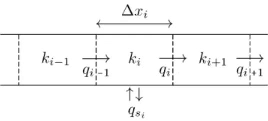
Fig. 1. Space discretization
integration of the effects of adversary weather. The PHD filter is implemented based on a Sequential Monte Carlo algorithm. Indeed, common traffic estimation issues can be tackled by the attractive properties of PHD filter, especially in dealing with clutter and multiple traffic flows (considering weather conditions). In most of the existing PHD filters, the clutter is modeled as a Poisson random finite set with a given intensity. The clutter intensity is characterized as a product of the average number of clutter (false alarm) points per scan and the probability density of clutter spatial distribution.
This work applies the PHD filter jointly with a constant velocity model for estimation of trajectories. In contrast to [2], in which authors estimate road traffic intensity based on mobile vehicles’ coordinates, we develop a PHD filter for traffic networks, and combine the CTM with the PHD filter. Its performance is evaluated over a real-world study case.
III. METHODOLOGY
A. Macroscopic traffic model
In this study, the traffic model used is the well-known first order Lighthill-Whitham-Richards (LWR) model in its sending-receiving cell version of Daganzo [5], which is based on hydrodynamic analogy describing the behavior of the traffic flow. Let us recall it briefly in its discrete version, with application to a simple section (as shown on Figure 1). The motorway section is divided into n cells of length∆xi. The
cell densities,kifor celli, and flows,qifor flow between cell
iandi+1, are updated every∆tN interval where the subscript
N stands for numerical.
The complete model is composed of two equations. The first equation is the conservation equation. The second equation is the flow equation which consists of the demand-supply flows, i.e. the resulting flow in cell i at time t will be the minimum between cell i+ 1 supply Σi+1(t) and the cell
i demand Γi(t). Note that the Stochastic Cell Transmission
Model (SCTM) developed by Sumalee et al., [18], extends the CTM to consider both supply and demand uncertainties. The numerical time step is taken as a sub-multiple of the observation time step fulfilling numerical conditions.
The state vector (of length2n+ 1) to be estimated consists of the flows and densities in the ncells of the section:
xt= k1(t), . . . , kn(t), q0(t), . . . , qn(t) T
, (1) whereT denotes the transpose operator.
The inputs ut of the system are the demand upstream and
the supply downstream of the considered section and other
perturbations (incidents, work zones). The state equation is then written as follows:
xt+1=f(xt, ut), (2)
wheref is a complex and highly nonlinear function with no straightforward analytical form.
The state equation (2) is completed by an (linear) obser-vation equation, which maps measurements, yt, and the state
vector of the system:
yt=Cxt, (3)
whereCis a real matrix consisting of rows whose elements are all zero except for the element corresponding to the position of the sensor delivering a measurement.
As there are uncertainties in both the measurements and the model, the complete dynamical model is given by
xt=f(xt−1, ut−1) +wt,
yt=Cxt+vt,
(4) where wt and vt are Gaussian noises of null mean and
variance-covariance matrix respectively Qt andRt.
B. The particle PHD filter for traffic state estimation 1) Overview: The PHD filter is a multiple target filter for recursively estimating the number and the state of a set of targets given a set of observations. It works by propagating in time the first moment (called intensity function or PHD function) associated with the multi-target posterior [10]. Multi-target tracking is a common problem in many applications. The literature in this area is spread and the state-of-art and methodology are well summarized in [11]. Recently, one article has been concerned by traffic modeling issues [2], and the potential for real-time traffic state estimation has been investigated in Canaudet al., [4].
In [7] and [12] the authors highlighted the fact that the PHD filter outperforms the standard approaches such as the Kalman Filter (KF), Particle Filter (PF) or the Multiple Hypothesis tracking (MHT). One can find many implementations of the PHD filter either via the sequential Monte Carlo (SMC) method [21], [24] or using finite Gaussian mixtures (GM) [22], [23].
The GM method is attractive because it provides a closed form algebraic solution to the PHD filtering equation, with the state estimate (and its covariance) easily accomplished. However, the GM method is based on somewhat restrictive assumptions that single-object transitional densities and like-lihood functions are Gaussian, and that the probability of survival and the probability of detection are homogenous ([11] [22]). The SMC method imposes no such restrictions and should therefore provide a more general framework for PHD filtering, even though it is also affected by different issues [11].
Beginning with Sidenbladh [16] and Zajic and Mahler [25], most researchers have implemented the PHD filter using SMC methods. SMC techniques were originally devised to approx-imate probability densities and the single-target Bayes filter.
Consequently, they must be modified for use with the PHD filter. This is because first: (i) the PHD is not a probability density function, and (ii) the PHD filter equations are more complex than the single-target Bayes filter equations.
Despite these differences, the SMC approximation carries over to the PHD filter relatively easily (with the exception of regularization). Particles represent random samples drawn from a posterior PHD. Particles are supposed to be more densely located where targets are most likely to be present. As with single-target SMC filtering, the basic idea is to propagate particles from time step to time step so that this assumption remains valid. The implementation is introduced in [21]. Then some improvements have been proposed in [13] and [15].
2) General formulation: The purpose of this section is to introduce the general formulation of a probability hypothesis density in the random finite set framework for multiple-target filtering. In this context multiple-targets and measurements are considered as random sets (random in values and also in number of values). From time step to time step, some of these targets may disappear. The surviving targets evolve to their new states and new targets may appear. Due to imperfections in the detector, some of the surviving and newborn objects may not be detected, whereas the observation set Yt may include
false alarm detection.
The concept of PHD filter then requires to recursively esti-mate the set of states of allnttargets,Xt={xt,1, . . . , xt,nt} that are present at time t given random measurements Yt =
{yk,1, . . . , yk,mk} for all k up to time t. In the next parts of the paper, we abusively use x to denote the multi-target vector state, in order to simplify notation and without loss of generality since the context gives enough information about which vector is used. The underlying idea of the PHD filter is to propagate a suitable density functionD(x)in the target state space χ ⊂ Rn (n = dim x). The PHD is a density
function but not a probability density function, such that, for any region S ⊆ χ, the expected number of targets in S is given by
n(S) =
Z
S
D(s)dx, (5) i.e. by integration of D(·)over S.
Let’s D(·) be the PHD function and Dk|k be the PHD
function at time k based on the set Yk of measurements till
time instantk. The objective of PHD filter is time propagation
Dk−1|k−1(x)→Dk|k−1(x)→Dk|k(x). (6)
Before presenting the predictor and corrector equations, we introduce some assumptions and notations. The PHD filter presumes some multi-target motion model. More precisely, target motions are statistically independent. Targets can disap-pear from the scene. New targets can be spawned by existing targets; and new targets can appear in the scene independently of existing targets. These possibilities are described as follows.
• Motion of individual targets: fk+1|k(x|x0) is the single
target Markov transition density.
• Probability of surviving:pS,k+1|k(x0)notedpS(x0)is the
probability that a target with statex0 at time step kwill
survive in time step k+ 1.
• Spawning of new targets by existing targets:bk+1|k(x|x0)
but as this phenomenon is negligible in our case, this asumptions is not included in this formulation compared to the general PHD recursion [11].
• Appearance of completely new targets: bk+1|k(x) is a
term characterising that new targets with state set xwill enter the scene at time stepk+ 1.
The PHD filter also presumes the standard multitarget measurements model. More precisely, no target generates more than one measurement and each measurement is generated by no more than a single target, all measurements are condition-ally independent of the target state, missed detections, and a multiobject Poisson false alarm process. These assumptions can be summarized as follows:
• Single-target measurement generation: Lk(y|x) is the
sensor likelihood function for observationy at time step
kand state x.
• Probability of detection:pD,k+1|k(x0)notedpD(x0)is the
probability that an observation will be collected at time step k+ 1 from a target with state x, if the sensor has state x0 at that time step.
• False alarm density: At time stepk+1, the sensor collects an average number λ= λk+1(x) of Poisson-distributed
false alarms, the spatial distribution is governed by the probability densityc(y).
With these notations, we now describe the basic steps of the PHD filter: initialization, prediction and correction.
1) PHD Filter initialization
Regarding the initialization step of the PHD filter i.e. the choice of D0|0(x), no special recommendations are
given in the litterature. One could choose this PHD initialization as a sum of Gaussians. Mahler, [11], em-phasizes that with no prior information about initial target position, an uniform PHD should be chosen. 2) PHD Filter predictor
At time step k, starting from Dk|k, one can derive a
formula for the predictive Dk+1|k, which can be found
in [10], defined as: Dk+1|k(x) =bk+1|k(x) | {z } birth targets + Z Fk+1|k(x|x0)Dk|k(x0)dx0, (7) where the PHD “pseudo-Markov transition density” is
Fk+1|k(x|x0) =pS(x0)fk+1|k(x|x0) | {z } persisting targets +bk+1|k(x|x0) | {z } spawned targets , (8) with the spawned target equal to zero in our study case. The predicted number of targets is therefore
Nk+1|k = Z
then we have, under the non restrictive assumption of no spawning, Dk+1|k(x) =bk+1|k(x)+ Z pS(x0)fk+1|k(x|x0)Dk|k(x0)dx0. (10) 3) PHD Filter corrector
From the previous step, one has the predicted PHD
Dk+1|k(x), given by (10). At time stepk+1, one collects
a new observation setYk+1 ={y1, . . . , ym}and requires
a formula for the data updated PHD Dk+1|k+1(x).
According to Mahler, [10], the PHD corrector step is
Dk+1|k+1(x) =Lk+1(y|x)Dk+1|k(x), (11)
where the “PHD pseudo-likelihood” function is defined by Lk+1(y|x) = 1−pD(x)+ pD(x) X y∈Y Lk(y|x) λc(y) +R pD(x)Lk(y|x)Dk+1|k(x)dx . (12) Then we have, Dk+1|k+1(x) = [1−pD(x)]Dk+1|k(x)+ X y∈Y pD(x)Lk(y|x)Dk+1|k(x) λc(y) +R pD(x)Lk(y|x)Dk+1|k(x)dx . (13) C. Clutter intensity
In Bayesian multi-target filtering knowledge of parameters such as clutter intensity and sensor field-of-view are of critical importance. Significant mismatches in clutter and sensor field of view model parameters result in biased estimates. In addi-tion to the non-linearity, process and measurement noise, the two main sources of uncertainty which constitutes significant challenges in multi-target filtering are clutter and detection. Clutter are spurious measurements that do not belong to any target.
An unknown and non-homogeneous clutter intensity is accommodated in [9] by dropping the standard Poisson as-sumption for false alarms, and modelling individual clutter returns based on individual clutter targets or generators. Each clutter generator is analogous to an actual target, in the sense that clutter generators have their own separate models for births and deaths as well as transition, likelihood and detection or missed detection. However, the two types of clutter and actual targets are distinct, and cannot evolve into the other type. The intuition here is that the clutter generators will dynamically distribute themselves around the state space to explain the prevailing false alarm conditions.
However, since in traffic modeling and state estimation problem the use of the PHD filter is a new concept, the first step should be to investigate if some simple assumptions as Uniform or Poisson distribution is far away from the ground
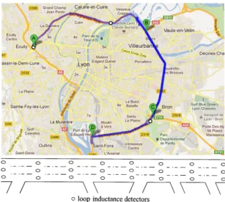
Fig. 2. Test site section (B→ C) divided into 7 cells and its detector configuration
truth, or if it possible to choose an adaptative methodology, automatically estimating the clutter intensity ([17]).
IV. EXPERIMENTAL RESULTS
A. Site and collected data
The test site is the urban freeway located at the Eastern part of Lyon’s ring road (point A to D on figure 2), which consists of three lanes between km point B and km point C (5.6km long), [3], [14]. Traffic data were provided by the urban motorways’ operator CORALY and collected in 2007 from 8 loop sensors.
The upstream demand and the downstream supply and bal-ances from a rainy day are used. The profiles of these external actions on the motorway system come from the real data of highway flow measurements in March 2007, on one weekday (Tuesday). The motorway section under consideration is the most frequently congested part. The upstream flow comprises the flow from North-West Lyon and the on-ramp from the Geneva freeway (point B). Therefore, the upstream demand presents high values on classical peak hours in the morning and at the end of the afternoon.
According to the section configuration, the space discretiza-tion of our traffic model has been carried out in such a way that the discretized cells are the segments between two consecutive sensors (Figure 2). Hence, we have 7 cells and 8 sensors. In this urban motorway section, three on and off-ramps are located on cells 3, 5 and 6. Therefore, in the traffic model, source terms have to be considered in these cells. The balance on versus offramp movements are shown in figure 3 as well as upstream demand.
B. Hypothesis, models parameters and filter considerations
From previous works, e.g. [14], the calibration of the fundamental diagram for this test site under rainy conditions (which is the case of the selected day), is achieved with the following parameters:
Fig. 3. Upstream demand and the balance ramp movements
1) Critical density:kc=100 [veh/km];
2) Maximum density: kM=300 [veh/km];
3) Maximum flow: qM=138 [veh/min].
The variance matrices needed in the estimation method also have to be selected. For the flow measurement uncertainty we have chosen a standard deviation of σR=1.5 [veh/min]
(consistent with empirical analysis conducted on the raw data collected on this network). Hence, the noise variance matrix is then defined by:Rt=diag(σ2R). Regarding the uncertainty
of the state equation, we assume the choice that the model is as robust as the measurements, meaning that the standard deviation of state vector flow part is the same as measurements one (σQ=1.5 [veh/min]). The density magnitudes are much
smaller than those giving the flow; therefore the standard deviation of the density part of the state vector is chosen to be:
σk =σQ×
kc
qM
= 0.0011 [veh/m] (14) Thus, thenfirst diagonal elements of theQmatrix are equal toσ2
k whereas the (n+ 1) last ones are equal toσ2Q.
Regarding the filters, the particle PHD filter uses the fol-lowing parameters:
1) Probability of detection:Pd=0.98;
2) Number of particles: Np=400;
3) Number of birth particles:Nb=250;
4) Number of clutter (false alarm): Nc=1.
We assume for the particle initialization a “Uniform PHD”. Moreover, as the newborn object particles need to cover the entire state-space with reasonable density for the SMC-PHD filter in order to work properly, [13], the birth density is driven by measurements following a uniform distribution. Further, it is supposed that, at each time instantt, on averageNc clutter
measurements are generated with an uniform distribution in the measurement space.
C. Performance evaluation
In order to evaluate performance of PHD filter for real-time traffic state estimation, the proposed methodology has been carried out. The assimilation was performed by two methodologies: (i) Particle filter and (ii) SMC-PHD filter, both under the same conditions (CPU time, filter and model parameters). Finally, we compare the flow estimates obtained from both filters and for each sensor location.
The simulation has been conducted as follows. First, it is supposed that measurements at some boundary cells are available. Then, it is assumed that the upstream demand and
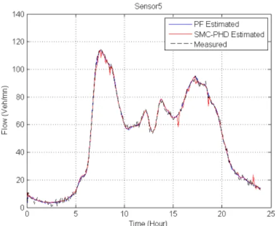
Fig. 4. Actual versus estimated flows for the fifth sensor. Dot-lines represent real measured flows and blue and red solid line are respectively PF and SMC-PHD estimates
downstream supply are known with a certain probability of detection and false alarms, as well as the ramp balances of in and out flows. Then we estimate by the two proposed methodologies the state vector of densities and flows. For comparison purposes, estimated versus actual traffic flows have been depicted for both estimation engines (see figure 4). Root Mean Square Error (RMSE) is used as a measure of the performance. Namely, for each time step and each sensor, we compute: RM SEi= 1 NsNt Ns X j=1 Nt X k=1 ˆ yi,j(tk)−yj(tk) 2 , (15) where the subscript i =PF or PHD, Ns is the number of
sensors, Nt the number of time step and yˆi,j(tk) the traffic
flow estimates fori, sensorj at timetk.
Since noises are unknown with real data, first conclusions about the two methodologies could be subject to criticism. For example, if measurements if measurments are far from the real conditions, the less the RMSE, the worst the method. To prevent this, and following the work of Canaudet al., [4], we choose to perform the study on simulated data instead of real data. The aim is that when we form the differenceyˆ−y, we can easily see the error in % and then see the performance for all filters with respect to the ground truth data.
For setting up the simulation scenario, the typical days upstream demand and downstream supply and balances of ramp movements introduce before were used. In other word, simulated data were derived from the real one. The model used to simulate data is the same as the one used in the filters in which the level of noises of the simulated data is defined by the diagonal ofQ. Results are presented in table I.
As one can see, with only boundaries conditions, both esti-mates are quite similar, and close to the actual measurements with a noticeable PHD overperformance:RM SEP F=3.44 and
RM SESM C−P HD=3.29. However, PHD estimates appear
smoother that those given by PF, which can be an interesting feature if we look at the confidence interval of estimates.
TABLE I
RMSEOF THE ESTIMATIONS WITH SIMULATED DATA
cell 1 cell 2 cell 3 cell 4 sensor sensor sensor sensor
RM SEP F 1.3942 2.0524 2.0708 2.0420
RM SEP HD 1.9191 1.4859 1.6333 2.8381
cell 5 cell 6 cell 7 cell 8 sensor sensor sensor sensor
RM SEP F 1.9516 1.8819 2.1413 1.0018
RM SEP HD 2.3989 1.3884 1.1386 0.8493
Thus, PHD filter performed better than PF. Finally, focusing on the transition regime (from free flow to congestion and conversely), PHD detects changes in traffic conditions better.
V. CONCLUSIONS
This paper develops a PHD filter for traffic state estimation with an appropriate clutter intensity. It is implemented based on a SMC algorithm. Its performance is evaluated over a real-world study case. The results are compared with the generic PF, well recognized to solve traffic state estimation problems. The results show the potential of the PHD filter to be applied to traffic state estimation and lay the cornerstone for the clutter intensity feature. The results demonstrate that the PHD filter outperforms the particle filter on this real study case. Secondly, it opens new avenues for PHD filter research in traffic control, showing useful potential. The PHD filter can be especially powerful in dealing with multiple traffic flows. Specifically, this work can be extended with more complex models to adversary weather conditions (which means more clutter in the data), including switching state space models as developed in [3] or [19] in order to adapt the traffic state estimation according to weather or traffic conditions. Multiple data sources can also be considered since the PHD filter is relevant in multi-target multi-source tracking. One can consider urban traffic and the estimation of other information such as travel time under various noise uncertainties.
In conclusion, this first step in using the PHD filter for traffic estimation issues shows the potential use of such a tool. Some features have still to be investigated now, like the likelihood function, the calibration of some parameters: rate, resampling improvement, detection profile. The question of clutter intensity has to be reconsidered in order to automati-cally adapt itself. However, this filter has a great interest, with no doubt, and definitively needs more consideration for future traffic applications.
ACKNOWLEDGMENTS
This work is part of COST action TU0702 research activi-ties: Real-time Monitoring, Surveillance and Control of Road Networks under Adverse Weather Conditions [6]. The authors would like to thank CORALY (Lyons urban motorways man-agers) for providing them with real traffic data.
REFERENCES
[1] M. Arulampalam, S. Maskell, N. Gordon and T. Clapp, A tutorial on particle filters for online nonlinear/non-Gaussian Bayesian tracking, IEEE Transactions on Signal Processing,50(12), 174–188 (2002).
[2] G. Battistelli, L. Chisci, S. Morrocchi, F. Papi, A. Benavoli, A. Di Lallo, A. Farina and A. Graziano,Traffic intensity estimation via PHD filtering, In Proc. 5th European Radar Conf., Amsterdam, The Netherlands (2008). [3] R. Billot, N-E. El Faouzi, J. Sau and F. De Vuyst,Integrating the Impact of Rain into Traffic Management: Online Traffic State Estimation Using Sequential Monte Carlo Techniques, in Transportation Research Records : Journal of the Transportation Research Board,2169, 141-149 (2010). [4] M. Canaud, L. Mihaylova and N-E. El Faouzi, Probability hypothesis
density filter for real-time traffic state estimation and prediction, submit-ted to the Network and Heterogeneous Media special issues (2012) [5] C. Daganzo, The cell transmission model: A dynamic representation of
highway traffic consistent with the hydrodynamic theory, Transportation Research B,28(4), 269–287 (1994).
[6] N-E. El Faouzi and B. Heilmann Ed.Real Time Monitoring, Surveillance and Control of Road Networks under Adverse Weather Conditions: Advances in modeling and weather-sensitive traffic management, The TU0702 COST Action. ISBN 978-2-85782-699-6 ISSN 0768-9756. July 2012, Les collections de l’lNRETS.
[7] R. Juang and P. Burlina, Comparative performance evaluation of GM-PHD filter in clutter, In Proc. FUSION (2009).
[8] J. Lebacque, The Godunov scheme and what it means for first order traffic flow models, In Proc. of the 13th ISTTT (1996).
[9] F. Lian, C. Han and W. Liu, Estimating Unknown Clutter Intensity for PHD Filter, Ieee Transactions On Aerospace And Electronic Systems,
46(2010).
[10] R. Mahler, Multitarget Bayes filtering via first-order multitarget moments, IEEE Transactions on Aerospace and Electronic Systems,39(4), 1152–1178 (2003).
[11] R. Mahler, Statistical multisources multitarget information fusion, Artech House, 2007.
[12] K. Panta, B. Vo, S. Singh and A. Doucet,Probability hypothesis density filter versus multiple hypothesis tracking, In Proc. SPIE (2004). [13] B. Ristic, D. Clark and B. Vo,, Improved SMC implementation of the
PHD filter, In Proc. of the 13th International Conference on Information Fusion, Edinburgh, UK (2010).
[14] J. Sau, N-E. El Faouzi and O. De Mouzon, Particle-filter traffic state estimation and sequential test for real-time traffic sensor diagnosis, In ISTS’08 Symposium, Queensland (2008).
[15] M. Schikora, A. Gning, L. Mihaylova, D. Cremers and W. Koch, Box-Particle PHD Filter for Multi-Target Tracking, IEEE Trans. on Aerospace and Electronic Systems, under review (2012).
[16] H. Sidenbladh, Multi-target particle filtering for the probability hypothesis density, In Proc. 6th Int’l Conf. on Information Fusion, Cairns, Australia (2003).
[17] R.L. Streit, L.D. Stone,Bayes derivation of multitarget intensity filters, Int. Conf. Information Fusion (2008).
[18] A. Sumalee, R.X. Zhong, T.L. Pan, and W.Y. Szeto, tochastic cell transmission model (SCTM): a stochastic dynamic traffic model for traffic state surveillance and assignment, Transportation Research Part B,45(3), 507–533 (2011).
[19] X. Sun, L. Munoz and R. Horowitz, Highway traffic state estimation using improved mixture Kalman filters for effective ramp metering control, In Proc. of th 42nd IEEE Conf. on Decision and Control, Maui, Hawaii, USA (2003).
[20] J. Sussman, Introduction to Transportation Problems, Artech House, Norwood, Masachussets, 2000.
[21] B. Vo, S. Singh and A. Doucet, Sequential Monte Carlo methods for multi-target filtering with random finite sets, IEEE Trans. Aerospace and Electronic Systems,41(14), 1224–1245 (2005).
[22] B. Vo and W. Ma,The Gaussian mixture probability hypothesis density filter, IEEE Trans. Signal Processing,54(11), 4091–4104 (2006). [23] B-T. Vo, B-N. Vo and A. Cantoni, Analytic implementations of the
cardinalized probability hypothesis density filter, IEEE Trans. Signal. Processing,55(17), 3553–3567 (2007).
[24] N. Whiteley, S. Singh and S. Godsill,Auxiliary particle implementation of the probability hypothesis density filter, IEEE Trans. on Aerospace and Electronic Systems,46(3), 1437–1454 (2010).
[25] T. Zajic and R. Mahler, A particle-systems implementation of the PHD multitarget tracking filter, In Sign. Proc., Sensor Fusion, and Targ. Recogn., Bellingham (2003).