Comparisons of Reflectivities from the TRMM Precipitation
Radar and Ground-Based Radars
JIANXIN WANG1,2 AND DAVID B. WOLFF1,2
1 Science System and Applications, Inc., Lanham, Maryland 2 NASA Goddard Space Flight Center, Greenbelt, Maryland
Popular Summary
The precipitation radar (PR) aboard the Tropical Rainfall Measuring Mission (TRMM) satellite is the first quantitative space-borne weather radar dedicated to
measuring tropical precipitation from space. Given the TRMM’s decade long and highly successful operation, it is now possible to provide quantitative comparisons between ground-based radars (GRs) with the space-borne PR with greater certainty over longer time scales in various tropical climatological regions. Researchers have shown that the PR is consistently able to measure reflectivity with absolute calibration accuracy better than ±1 dB. Thus, the PR can serve as a consistent reference to calibrate GRs, and to detect inconsistencies between adjacent GRs. On the other hand, the PR has a relatively low sensitivity and its signal can be substantially reduced by heavy rain, whereas the GRs
have a higher sensitivity and operate at less-attenuating frequencies. Hence, GRs can in turn be used to check the PR rain detection ability and attenuation correction algorithm performance.
This study develops an automated methodology to match and compare simultaneous TRMM PR and GR reflectivities at four primary TRMM Ground
Validation (GV) sites: Houston, Texas (HSTN); Melbourne, Florida (MELB); Kwajalein, Republic of the Marshall Islands (KWAJ); and Darwin, Australia (DARW). Because of differences in scan geometries and resolutions for the PR and GR, it is necessary to resample data from each instrument into a three-dimensional Cartesian coordinate system. Comparisons suggest that the PR suffers significant attenuation at lower levels especially in convective rain. The attenuation correction performs quite well for convective rain but appears to slightly over-correct in stratiform rain. The PR and GR observations at HSTN, MELB and KWAJ agree to about ±1 dB on average with a few exceptions, while the GR at DARW requires +1 to -5 dB calibration corrections. One of the important findings of this study is that the GR calibration offset is dependent on the reflectivity magnitude. Hence, we propose that the calibration should be carried out using a regression correction, rather than simply adding an offset value to all GR reflectivities.
This methodology is developed towards TRMM GV efforts to improve the accuracy of tropical rain estimates, and can also be applied to the proposed Global Precipitation Measurement and other related activities over the globe.
Comparisons of Reflectivities from the TRMM Precipitation
Radar and Ground-Based Radars
JIANXIN WANG1,2 AND DAVID B. WOLFF1,2
1 Science System and Applications, Inc., Lanham, Maryland 2 NASA Goddard Space Flight Center, Greenbelt, Maryland
Revised manuscript
Submitted
Journal of Atmospheric and Oceanic Technology August 2008
_____________
Corresponding author address: Jianxin Wang,
ABSTRACT
Given the decade long and highly successful Tropical Rainfall Measuring Mission (TRMM), it is now possible to provide quantitative comparisons between ground-based radars (GRs) with the space-borne TRMM precipitation radar (PR) with greater certainty over longer time scales in various tropical climatological regions. This study develops an automated methodology to match and compare simultaneous TRMM PR and GR
reflectivities at four primary TRMM Ground Validation (GV) sites: Houston, Texas (HSTN); Melbourne, Florida (MELB); Kwajalein, Republic of the Marshall Islands (KWAJ); andDarwin, Australia (DARW). Data from each instrument are resampled into a three-dimensional Cartesian coordinate system. The horizontal displacement during the PR data resampling is corrected. Comparisons suggest that the PR suffers significant attenuation at lower levels especially in convective rain. The attenuation correction performs quite well for convective rain but appears to slightly over-correct in stratiform rain. The PR and GR observations at HSTN, MELB and KWAJ agree to about ±1 dB on average with a few exceptions, while the GR at DARW requires +1 to -5 dB calibration corrections. One of the important findings of this study is that the GR calibration offset is dependent on the reflectivity magnitude. Hence, we propose that the calibration should be carried out using a regression correction, rather than simply adding an offset value to all GR reflectivities.
This methodology is developed towards TRMM GV efforts to improve the accuracy of tropical rain estimates, and can also be applied to the proposed Global Precipitation Measurement and other related activities over the globe.
1. Introduction
The precipitation radar (PR) aboard the Tropical Rainfall Measuring Mission (TRMM) satellite is the first quantitative space-borne weather radar dedicated to measuring tropical precipitation from space (Simpson et al. 1996). Both internal and external calibrations of the PR have been performed to ensure accurate and stable rain measurements. The internal calibration checks the performance of the receiver systems by changing the input power level, and the external calibration checks overall
performance using an active radar calibrator located at a ground calibration site in Japan (Takahashi et al. 2003). Both calibrations have shown that the PR is consistently able to measure reflectivity with absolute calibration accuracy better than ±1 dB (Kawanishi et al. 2000; Kozu et al. 2001; Takahashi et al. 2003). Thus, the PR can serve as a consistent reference to calibrate ground-based radars (GRs), and to detect inconsistencies between adjacent GRs (Anagnostou et al. 2001; Schumacher and Houze 2001; Houze et al. 2004). On the other hand, the PR operates at an attenuating frequency of 13.8 GHz (Ku-band) and has a low sensitivity threshold of 18 dBZ
(
http://www.eorc.jaxa.jp/TRMM/documents/PR_algorithm_product_informa
tion/pr_manual/pr_manual_v6.pdf
), whereas the GRs operate at less-attenuating frequencies (such as S-band) and with higher sensitivity. Hence, GRs can be used to check the PR attenuation correction algorithm performance and rain detection ability (Bolen and Chandrasekar 2000; Schumacher and Houze, 2001; Liao et al. 2001).Calibration uncertainty is possibly the most severe problem in generating accurate rainfall products from radar observations. For example, a calibration offsetof 2 dB could contribute an uncertainty of 30% in the monthly rainfall estimation (Houze et al. 2004). It
is therefore necessary to develop an operational system for determination of the GR calibration bias for TRMM Ground Validation (GV) efforts.
A variety of approaches have been developed to address the calibration issue through cross validation of the PR and GRs. These approaches can be classified in two categories: grid-matching methods (GMM; Bolen and Chandrasekar 2000; Heymsfield et al. 2000; Anagnostou et al. 2001; Liao et al. 2001) and area-matching methods (AMM; Schumacher and Houze 2000; Houze et al. 2004). The GMM derives the calibration offset asthe mean difference between the two instruments based on grid-by-grid
reflectivity comparisons, whereas the AMM derives the offset via matching the area echo coverage seen by the GR (at reflectivities greater than a specified threshold) to the echo coverage observed by the PR. Houze et al. (2004) compared the calibration corrections of the GMM (from Bolen and Chandrasekar 2000) against the AMM (from Schumacher and Houze 2000), and found substantial differences.
Both above methods are labor-intensive due to numerous subjective decisions and selection of large overlapping echo areas from coincident PR and GR observations. Moreover, the results from these analyses may be subject to increased uncertainty
because they are based on individual overpasses in one or just a few years. The 10+ years of successful TRMM operations makes it possible for quantitative calibrations of GRs to be obtained over longer time periods and with greater certainty in various climatological regions. This study develops an automated operational system to determine GR
calibration corrections for four primary TRMM GV sites: Houston, Texas (HSTN); Melbourne, Florida (MELB); Kwajalein, Republic of the Marshall Islands (KWAJ); and Darwin, Australia (DARW). We compare radar reflectivities from the PR and GRs, and
also use GRs to check the PR attenuation correction. We begin with a discussion of the PR and GR data, and the data resampling method. This is followed by the methodology applied to match the resampled GR and PR data. Comparisons of the PR and GR reflectivities are provided in section 4. Section 5 presents the GR calibration correction, which is followed by section 6, comparisons between the GMM and AMM. Percentages of missed PR echoes and rainfall due to PR’s low sensitivity are presented in section 7. We end with summary and conclusions in section 8.
2. Data and resampling method
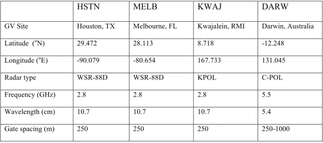
This study uses the GR observations and PR subset data over four primary TRMM GV sites: HSTN, MELB, KWAJ and DARW. Locations and general
characteristics for GRs at these four sites are provided in Table 1. Readers interested in
learning more about GRs and their operations may refer to Crum et al. (1993),
Schumacher and Houze (2000) and Wolff et al. (2005).The data cover the period 1998 to 2007 for HSTN and MELB, 2000 to 2007 for KWAJ, and 1998 to 2003 for DARW. We note that the GR at DARW is operated only during rainy seasons (November-April) each year. After 2003, DARW data are not available. The latest version-6 PR attenuation-corrected reflectivity from TRMM Standard Product (TSP) 2A-25 is compared with the latest version GR reflectivity from TSP 2A-55. The latest 2A-55 for HSTN, MELB and DARW is version 5, and the latest 2A-55 for KWAJ is version 7. The GR at KWAJ before 2000 was too unstable to generate the version-7 reflectivity product.
TSP 2A-55 has undergone many improvements since TRMM launch in
by the “bulk-adjustment” technique that forces agreement between radar reflectivity and gauge rain rates (Robinson et al. 2000; Marks et al. 2000; Wang et al. 2008). In version 5, the “bulk-adjustment” technique was replaced with the Window Probability Matching Method (WPMM; Rosenfeld et al. 1994); WPMM statistically matches radar to rain gauge data for derivation of Ze-R lookup tables. Version 6 is an interim GV product in which the Relative Calibration Adjustment (RCA; Silberstein et al. 2008) was applied without accounting for changes in antenna elevation, while version 7 incorporated both RCA and antenna elevation angle corrections. A description of GR version history can be found in Marks et al. 2008 (submitted).
The comparison between the PR and GR is conducted for different rain types (stratiform and convective rain), and over different surfaces (ocean, land and coast). The rain type classifications are taken from TSP 2A-54 for GRs and TSP 2A-23 for the PR. The surface type classifications are from TSP 2A-25. TSP 1C-21 (the PR reflectivity without attenuation correction) is employed to check the PR attenuation correction accuracy. A detailed description of TSPs is available at
http://tsdis.gsfc.nasa.gov/tsdis/tsdis_redesign/SelectedDocs.html.
TSP 2A-55 contains three-dimensional reflectivities from each GR. They are instantaneous reflectivities interpolated from the GR spherical coordinate system (azimuth, elevation, and range) into the three-dimensional Cartesian coordinate system centered at each GR with a vertical resolution of 1.5 km to a height of 19.5 km, and a horizontal resolution of 2 km with covering range to 300 km. The National Center for Atmospheric Research (NCAR) software program known as “The Sorted Position Radar INTerpolation” (SPRINT; Mohr and Vaughan 1979) is used for the interpolation.
TSP 2A-25, known as the PR profile, is composed of the attenuation-corrected reflectivity and rain-rate profiles for each PR scan ray. The PR attenuation correction is derived from a hybrid method of the Hitschfeld-Bordan iterative scheme (Hitschfeld and Bordan 1954) and surface reference technique (Iguchi and Meneghini 1994). The beam-filling correction is also performed in 2A-25 attenuation-corrected reflectivities. Details of the 2A-25 algorithm are provided in Iguchi et al. (2000).
TRMM was originally stationed at an orbit of 350 km shortly after its launch on 27 November 1997, and then boosted to a new orbit of 402.5 km after it finished six burn pairs from 7 to 24 August 2001. The PR on board TRMM scans 17° to either side of nadir at intervals of 0.71° in the cross-track direction. This scan geometry gives 49 rays sampled over an angular sector of 34°, or a swath width of 214 km (246 km after the boost) at the earth surface, with a field-of-view (FOV) diameter of about 4.3 km (5.0 km after the boost) at the nadir. The FOVdiameter slightly increases towards the maximum scan angle (17°) and slightly decreases towards the tropopause. The PR pulse duration is 1.67µs, which corresponds to a range resolution of 0.25 km. In general, the PR data have horizontal resolution of ~ 4-5 km and range resolution of 0.25 km along the PR scan ray.
Note that the GR 2A-55 data are in Cartesian coordinates. Therefore, it is necessary to resample the PR data into Cartesian coordinates in order to make the grid-by-grid comparison. We set a three-dimensional Cartesian coordinate system centered locally at each GR with a horizontal extent of ±150 km and vertical range from 0 to 20 km. The Cartesian coordinate (x, y, z) of a PR sample can be calculated using following equations.
y = (R + r cos(
α
))(
φ
PR-
φ
GR)
(2)z
=
r cos(
α
)
(3)Where R is the Earth's radius at the GR latitude
R
=
(a
2cos(
φ
GR))
2+
(b
2sin(
φ
GR))
2(a cos(
φ
GR))
2+
(b sin(
φ
GR))
2 .Here a is the Earth's equatorial radius and equals 6,378.135 km; b is the Earth's polar radius and equals 6,356.750 km; r is the range distance from the PR sample to the earth ellipsoid along the PR scan ray; α is the PR scan angle relative to nadir ray (-17o≤α≤17o);
φ
PR and λPR are the latitude and longitude of the PR sample, respectively;φ
GR and λGR are latitude and longitude of the GR (the origin of the Cartesian coordinate system), respectively.Since the PR scan is confined to 17° off nadir, the range direction of each scan can be approximated as vertical to the earth surface. Therefore, the latitude and longitude of the center of the FOV at the altitude of the earth ellipsoid in TSP 2A-25 or 1C-21 can be approximated as the latitudes (
φ
PR) and longitudes (λPR) of the PR samples atdifferent range bins in the same scan ray. This approximation implies that an elevated PR sample at 10 km height with the maximum scan angle of 17o could be horizontally
displaced about 3 km from its earth surface position toward the nadir. This displacement is not a serious problem in some situations because it is usually less than the PR FOV size since the PR scan angle is smaller than or equal to 17° and most PR samples are lower than 10 km. However, sometimes, this displacement does shift the PR sample at a given grid point to its neighbor. The displacement or parallax needs to be corrected.
Figure 1 is an illustration of the displacement correction, where the footprint S1 of a PR sample S is displaced to S2 when the above approximation is used. The displaced distance S1S2= r sin (α), where r is the distance from S to S1, the same as in (1)-(3). For any two given PR rays RS1 and RS3, the scan plane RS1S3 is approximately perpendicular to the transverse plane S1PS3Q at the earth ellipsoid. The distances S1P and S1Q in the rectangle S1PS3Q can be calculated using (1) and (2) where (
φ
PR, λPR) and (φ
GR, λGR) are replaced with latitudes and longitudes of S1 and S3, respectively, thenS1S3= (S1P)2+
(S1Q)2.
The displacement (δx, δy) in x- and y-direction can be calculated as follows:
δ
x
=
S
1P
1=
S
1P
S
1S
2S
1S
3, (4)δy=S1Q1 =S1QS1S2 S1S3
. (5)
It should be noted that δx and δy could be positive or negative, which depends on eight cases for ascending or descending TRMM overpasses with scans from left to right side or from right to left side of the TRMM flight direction for all scan angles from -17 o to 0o or from 0o to 17 o. The displacement-corrected Cartesian coordinate (x+δx, y+δy, z) of a PR sample can be obtained by using (1)-(5).
The above resampling gives the Cartesian coordinates of PR samples at an approximate 4-5 km horizontal and 0.25 km vertical resolutions. However, the GR samples from TSP 2A-55 have the horizontal resolution of 2 km x 2 km and vertical resolution of 1.5 km. In order to make reasonable comparisons for the PR and GR, we
To avoid averaging biases associated with the logarithmic reflectivity (dBZ), we perform averaging on linear reflectivity (Z) instead of logarithmic reflectivity (dBZ). We convert 2A-25, 1C-21 and 2A-55 to linear units (Z), and average onto 4 km x 4km x 1.5 km grids. Here the linear averaging is performed in both horizontal and vertical directions for consistency. The linear averaging is easy to perform and is able to provide reasonable results (Heymsfield et al. 1983). Once averaging is complete, linear units are converted back to logarithmic.
3. Matching PR and GR samples
The data-resampling scheme can minimize calibration uncertainties due to the sampling resolution difference between the GR and PR. We resample all subset PR data for all overpasses over each GV site, and then resample the coincident GR data only when there are PR echoes during the overpasses. By doing so, large amounts of non-coincident or no-echo GR data are excluded in data resampling, as well as in the temporal and spatial matching between the PR and GR. Both GR and PR data are time-stampedat the start of each of their respective scans. Each GR volume scan lasts about 6 minutes whereas each PR scan only lasts about 0.6 second. Consequentially, the PR and GR data can be off in time by about 6 minutes. We set an 8-min time window (-1≤TimePR–
TimeGR≤7 min) and compare the gridded GR and PR reflectivities whenever both are in the same grid within this time window.
Using this matching scheme, the labor intensive and subjective selection of large overlapping echo areas for coincident PR and GR observations can be avoided, and the
comparison to only a few large overlapping echo areas with significant rainfall. Instead, it includes all matched grids, therebymaximizes the sample size and makes the comparison results statistically more robust.
4. Comparisons of GR and PR reflectivities
a. Profile comparisonsIn order to mitigate discrepancies due to different sampling and scan time
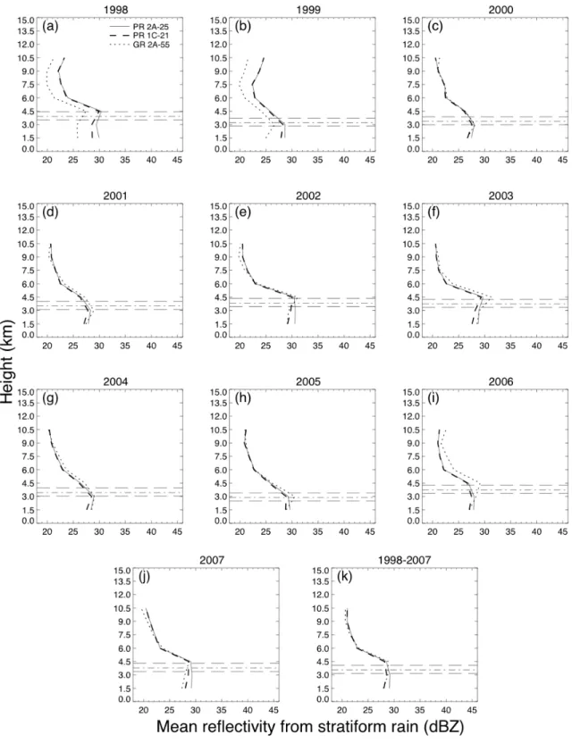
synchronization between PR and GR observations, we construct mean vertical reflectivity profiles for the PR and each GR by linearly averaging the matched data over each GR-centered 200 km x 200 km area at each altitude. The data are divided into two categories: stratiform and convective rain types. Because the PR has a low sensitivity of 18 dBZ, only reflectivities greater or equal to 18 dBZ are used in constructing PR and GR profiles for each of the four GV sites. Figure 2 shows the mean vertical reflectivity profiles for stratiform rain from GR 2A-55, corrected PR 2A-25 and
attenuation-uncorrected PR 1C-21 at HSTN from 1998 to 2007. Likewise, Fig. 3 shows the profiles for convective rainfall. Physically, stratiform rain is largely identified by the presence of the radar bright band, and convective rain is often identified by a large horizontal
reflectivity variation (Steiner et al. 1995). Different algorithms are used to identify rain types for the PR in TSP 2A-23 (Awaka et al. 1997) and for the GR in TSP 2A-54 (Steiner et al. 1995). The profiles in Fig. 2 and 3 comprise only those data grids where both the GR and PR rain types are the same. Figure 2 also shows the upper and lower boundaries of the radar bright band (horizontal sparse dashed lines) with the peak bright band in the middle. The bright band positions are calculated from TSP 2A-23 for stratiform rain only
when the bright band is detected. The PR is usually able to detect the bright band because of its fine vertical resolution (Durden et al. 2003). However, the bright band does need some correction because it does not always appear to be consistent with the peak
reflectivity from year to year (Fig. 2). The profiles are truncated to 10.5 km for stratiform and 13.5 km for convective rain type, respectively, because there are too few samples above the truncated heights to make statistically meaningful comparisons. At upper levels where the PR attenuation effect is minor, PR 2A-25 agrees well with PR 1C-21,
especially for stratiform rainfall above the bright band (Fig. 2). At lower levels, PR 1C-21 is significantly lower than PR 2A-25, especially for convective rainfall near surface (Fig. 3). The PR signal is significantly attenuated by cloud water, rain and partially melted hydrometeors during its passage from the cloud top to the surface. The average attenuation correction was as large as 8 dB as shown in Fig. 3a for convective rain at 1.5 km in 1998. Reflectivities from convective rain require more attenuation correction than from stratiform rain. On average, the 2A-25 algorithm for attenuation correction performs quite well for convective rain (Fig. 3) but appears to slightly over-correct in stratiform rain (Fig. 2).
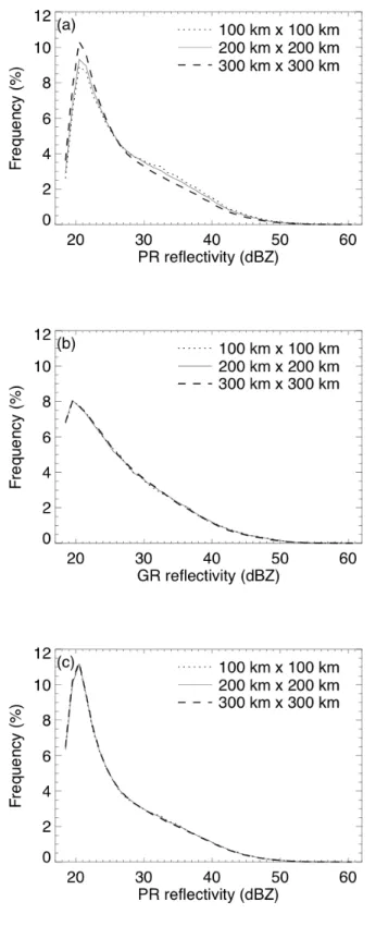
The average differences between PR 2A-25 and GR 2A-55 for all levels at HSTN from 1998 to 2007 shows that GR is 0.41, 0.41, 0.34 dB lower than the PR for stratiform, convective and all rain types, respectively. These differences are well within the PR’s precision of 1 dB. We also construct similar profiles by using data over GR-centered 300 km x 300 km and 100 km x 100 km areas, and find that the mean difference slightly decreases as the area increases. This is consistent with Figs. 4a, b, which show frequency distributions of all matched PR and GR reflectivities, disregarding rain and surface types
for different areas. Although the frequency distribution of all PR reflectivities (matched and unmatched dada) is area-independent (Fig. 4c), spatial and temporal matching between PR and GR samples more high PR reflectivity data, and the frequency of matched high PR reflectivity slightly decreases when the area increases (Fig. 4a), whereas the frequency distribution for the GR does not notably change (Fig. 4b). The slight change of the mean difference should not be due to the GR’s beam-filling effect that should increase with the data area. Thus, the change appears to result from the sampling of the PR data.
The GR was 1-3 dB lower than the attenuation-corrected PR during earlier
TRMM years (1998-99) (Fig. 2a, b and Fig. 3a,b). After 1999, the GR was in line with or a little higher than the attenuation-corrected PR, except for 2006 when the GR was about 1-2 dB higher than the PR. Comparing the profiles for the PR and the well-maintained and stable GR at MELB, we find no obvious difference between 1998-99 and 2000-2007. This demonstrates that the GR at HSTN experienced the temporal variation and the PR can serve as a calibration standard for the GR.
We also classify the PR and GR data according to different surface types: over land, ocean and coast, and find that the vertical reflectivity profiles for these types are similar.
b. Scatter comparisons
More detailed comparisons between the PR and GR can be performed on grid-by-grid basis via scatter plots. Using the attenuation-corrected PR reflectivity as a reference, we define the GR calibration offset O as follows:
O=RPR - RGR (6) where RPR and RGR are the matched reflectivities ≥18 dBZ from the PR and GR,
respectively. Whether RGR is lower or higher than RPR, we just need to add the positive or negative offset value O to the GR reflectivity to bring the GR in line with the PR. Figure 5 shows offset scatter plots classified according to rain type (stratiform and convective rain) or surface type (ocean, land and coast) at HSTN over the period from 1998 to 2007. The large scatter seen in Fig. 5 could be related to following:
1) The spatial and temporal matching between the PR and GR. The latitude and longitude of a PR scan ray in 2A-25 are calculated from the estimated surface range gate location where the return power reaches its maximum value (Kozu et al. 2001). Inaccuracy in the PR ray location can cause the grid mismatch relative to that of the GR. Temporal matching of PR and GR observations is often a more serious problem. As discussed in section 3, the PR and GR data can be off in time by about 6 minutes; consequently, poor comparisons can be expected for rapidly evolving and moving rain systems.
2) Resolution difference in PR and GR observations. The PR measures rainfall with the resolution of 4-5 km in horizontal and 0.25 km in vertical, whereas the GR measurements with the 0.25-km range resolution and variable vertical resolution. The GR beam width of 1.12o corresponds to the vertical resolution coarser than 2 km at a slant range of 100 km or farther from the GR. Both the PR and GR data are interpolated into 4km x4 km x 1.5 km grids in order to make reasonable comparisons. The data resampling could contribute to large scatters in Fig. 5.
3) Non-Rayleigh scattering effect at the PR frequency. High reflectivities are usually associated with densely distributed large particles. The backscattering cross sections of these large particles can be significantly different from the GR of 10.7-cm wavelength and the PR of 2.17-10.7-cm wavelength. This non-Rayleigh scattering effect can be simulated using the raindrop size distribution model. Bolen and Chandrasekar (2000) showed that the PR reflectivity could be up to 2 dB higher than the GR reflectivity for higher reflectivity of 40-50 dBZ because of the non-Rayleigh scattering.
4) Attenuation effect both in the PR and GR. The PR operates at a frequency of 13.8 GHz and suffers from significant attenuation in lower levels. Figures 2 and 3 show that the attenuation correction works well but far from perfect. Although the attenuation effect in the GR is often neglected, this effect also contributes to increase the discrepancy between the PR and GR reflectivities (Liao et al. 2001). 5) Non-uniform beam filling (NUBF) effect both in the PR and GR. The PR
measurements have horizontal resolution of ~ 4-5 km whereas convective rain often falls from cells smaller than 4-5 km. Therefore, the NUBF has a systematic effect on the PR reflectivity. The NUBF correction was performed in 2A25, but its validity is yet to be verified (Kozu and Iguchi 1999; Iguchi et al. 2000). Although the GR has good slant-range resolution, its vertical resolution decreases with increasing range. The NUBF effect in the GR can also misrepresent the reflectivity.
A comparison of Fig 5a with Fig5.b shows that the scatter for stratiform rain is much smaller than that for convective rain although the former has the double sample
size. The larger scatter in convective rain is related to the beam filling effect and the non-simultaneity between the PR and GR observations. The scatter plots for different surface types (Fig.5 c-e) display little difference except much smaller sample size for the type over coast. The positive offset in Fig. 5 is bounded to a linear line O=RPR -18 when RGR is at its minimum value of 18 dBZ so that O reaches its maximum value RPR -18. The negative offset is not obviously bounded but seems parallel to that linear line. Although the mean offset changes in a very narrow range from 0.27 dB over land (Fig. 5c) to 0.47 dB over coast (Fig. 5e), the individual offset can be in a very wide range from -30 to 30 dB at different reflectivity magnitudes. Higher reflectivities are prone to suffer larger positive offsets and vice versa. The positive and negative offsets sum to small mean offsets. The offset is dependent on the reflectivity magnitude, which is clearly revealed in different rain and surface types at HSTN in Figs. 5a-f. The dependence is expressed by linear regression models (solid lines) in Fig. 5. The scatter plots for all other GRs at MELB, KWAJ and DARW for entire data periods display similar features. The
magnitude dependence of the offset is related to the non-Rayleigh scattering effect, which results in the larger offset at higher reflectivity due to the shorter PR wavelength.
We also limit the data to at least 18 dBZ above the bright band in stratiform rain only for each year at each GR. The magnitude dependence of the offset is displayed in Table 2, which will be discussed in section 7. However, this dependence was not easily revealed in Anagnostou et al. (2001) because their analysis was only based on each of ten overpasses with small sample sizes.
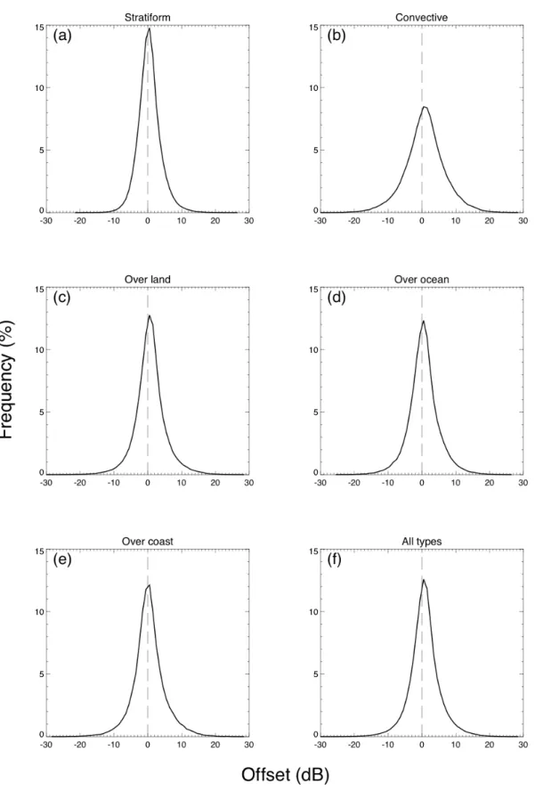
Figure 6 shows the frequency distribution of offsets Odefined in (6) for different rain and surface types at HSTN from 1998 to 2007. Figures 6a-f all have shapes similar to Gaussian distribution with means from 0.3 to 0.5 dB and standard deviations (STD) ranging from 3.5 dB for stratiform to 6.0 dB for convective rain type. The largest STD for the convective rain (Fig. 6b) is consistent with the widest scatter (Fig. 5b). As the profile and scatter comparisons discussed earlier, the frequency distributions for different surface types are similar.
Basing on the analyses in section 4a-c, we only use the matched GR and PR attenuation-corrected reflectivities at least 18 dBZ and above the bright band in stratiform rain type, regardless of surface types, for the determination of GR calibration offsets in section 5. These conditions constrain the comparison to most reliable data, minimize uncertainties caused by potential PR attenuation correction errors, and eliminate
uncertainties associated with high subgrid rainfall variability in convective rain type, and random effects because of rain type changes.
5. Calibration offsets
According to Fig. 5, the offset O is dependent on the reflectivity magnitude, which can be expressed by a linear regression model
) (RPR RPR b
O
O= + − . (7)
In (7), b is the regression coefficient; RPR is the PR reflectivity and RPR is its mean;
O
is mean offset given by(
)
∑
− = n PR GR R R n O 1 (8)where RGR are the GR reflectivity, and n is the sample size. Only the reflectivities
classified as stratiform, above the bright band, and at least 18 dBZ are used in (7) and (8). The coefficient b can be used to measure the dependence of calibration offset on the reflectivity magnitude. When the offset is dependent on the reflectivity magnitude (b≠0), individual GR reflectivity should be calibrated by adding its individual offset determined by (7), which can be called “the regression correction”. When the offset is independent of the reflectivity magnitude (b=0) or RPR is at its mean value
R
PR, thecalibration can be done by simply adding
O
to all GR reflectivities, which can be called “the mean difference correction”. The mean difference correction is a special case of the regression correction. The regression correction does not affect mean difference.Based on (7), it is clear that the mean of the offsets (O) from the regression correction is equal to the mean offsetO
from the mean difference correction.Table 2 lists yearly
O
, b andRPR
for HSTN, MELB from 1998 to 2007, KWAJ from 2000 to 2007, and DARW from 1998 to 2003. The dependence of calibration offset on the reflectivity magnitude changes from year to year and site to site. Differentregression calibrations should be individually applied to each GR reflectivity value. The yearly mean offsets were about ±1 dB at HSTN, MELB and KWAJ over the entire data periods, except at HSTN in 1998 and 1999, and MELB in 2002 when the offsets were about 2 dB. The GR at DARW required +1 to -5 dB calibration. Liao (2001) compared GR and PR reflectivities from 24 overpasses at MELB in 1998, and found that the GR was about 1 dB lower than the PR. This result is very close to our mean offset of 0.70 dB in Table 2 at MELB in 1998.
While the regression calibration should be used to get the GR offset, the mean difference calibration offset
O
between the PR and GR measurements can be used to systematically estimate the relative biases of the GR reflectivities at the mean reflectivity magnitude or in the case when the offset is not obviously dependent on the magnitude. However, only providing the mean offset value is not sufficient unless it is accompanied by its confidence interval. When the sample size is sufficiently large, the mean offset follows Gaussian distribution according to the central limit theorem. Hence, we can construct a Student’s t- test statistic (Wilks 1995) and derive that 100(1-α)% confidence interval ofO
is(O
−
t
α/ 2s
n
,O
+
t
α/ 2s
n
)
. (9)Here α is statistical significance level of 5%; tα/2is the 100(α/2)th percentile of the t-distribution with n-1 degree of freedom, and s is the sample STD of the individual O values:
∑
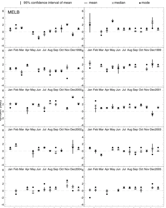
− − = n O O n s ( )2 1 1 . (10)Shown in Figs. 7-10 are the monthly and yearly offsets for GRs at HSTN and MELB from 1998 to 2007, KWAJ from 2000 to 2007, and DARW from 1998 to 2003. Some months are missing in Figs. 7-10 either because of a dearth of rainy PR overpasses or missing GR observations. For example, there is no offset plotted from August through Decemberin 2005 in Fig. 9 because the GR at KWAJ experienced multiple hardware failures during this period. GR data at DARW are available only during the rainy seasons. The mean offset and its 95% confidence interval, as well as the median and mode offsets,
are plotted in these figures. The vertical bar represents 95% confidence interval of the mean offset. A large confidence interval means large uncertainty of the estimated mean offset. As we can infer from (9), the mean offset can be subject to significant uncertainty because of the small sample size and large sample STD. Besides the mean, the mode and median can also be chosen to measure GR calibration offset. The mode is a specific value with the greatest occurrence in the frequency distribution. The median, or the 50th
percentile, is the value at the center of the data set. Unlike the mean, which is averaged from all data, the mode and median are less sensitive to a small number of outliers. However, the mode offset in Figs. 7-10 sometimes is quite different from mean and median offsets because the mode can be incorrectly presented in a rough frequency distribution with multiple peaks. This occasionally happens especially when the sample size is small.
One observation extracted from Figs. 7-10 is that the offset shows its noticeable spatial variation from site to site and temporal variation from month to month. This clearly indicates systematic differences of GR observations against PR measurements. Hence, the PR can be utilized as a consistent reference to calibrate various GRs.The GR at MELB (Fig. 8) is relatively stable with less month-to-month fluctuations in offsets during the ten years in comparisons with other GRs (Figs. 7, 9 and 10). The GR at DARW requires the most calibration corrections (Fig. 10).
The GR at KWAJ in the decade since TRMM launch experienced numerous radar calibration changes, which are partially available for review from the site logs maintained by the prior on-site contractor 3D Research Corporation. The changes from 1998 to 2001 were also listed in Houze et al. (2004). Unfortunately, logs at radar sites are often either
unavailable or lack sufficient detail information. The temporal offset variability is related to changes of the GR status, which could be the results of the maintenance of the radar azimuth and elevation motors, changes in scan strategy, or gradual degradation of the radar performance such as gain, loss, antenna, etc. The RCA technique was recently developed to monitor radar sensitivity fluctuations using statistical ensemble
characteristics of clutter area reflectivity (Silberstein et al. 2008). For version 7, eight years of KWAJ reflectivity data (2000-2007) were corrected using the RCA method, and the stability in reflectivity distributions was greatly improved over earlier versions (Marks et al. 2008). Both Fig. 9 and Table 2 show that the yearly offset for KWAJ version-7 2A-55 is on the order of ± 1 dB, which is around the estimated uncertainty of the PR.
Similarly, the GR offsets can also be estimated on overpass or daily basis. Daily, monthly and yearly results at HSTN, MELB, KWAJ and DARW are available from the TRMM GV website http://trmm-fc.gsfc.nasa.gov/trmm_gv.
6. Comparison of calibration corrections using GMM and AMM
The GMM compares the resampled grid data from the PR and GR. Bolen and Chandrasekar (2000) remapped simultaneous PR and GR reflectivity data to a GR-centered coordinate system with the horizontal resolution of 4 km x 4 km and vertical resolution equal to the GR beam width. Then the remapped data were averaged over the entire horizontal plane at each altitude. Comparisons of mean vertical profiles from the PR and GR were performed. This approach was also called “mean difference method” in Houze et al. (2004). Heymsfield et al. (2000) mapped PR and GR reflectivities to a densegrid representing the nadir beam and gate spacing of the airborne ER-2 Doppler radar. Anagnostou et al. (2001) projected instantaneous PR and GR reflectivity data into a common earth parallel three-dimensional Cartesian grid with the horizontal resolution of 5 km x5 km and vertical resolution of 2 km. Liao et al. (2001) interpolated PR and GR data to a common grid with 4 km x 4 km horizontal and 1.5 km vertical resolutions. Comparisons between the PR and GR in these past studies, as well as this analysis, are all performed on the grid basis, and can therefore be referred to as the GMM. They are similar, but technically different in almost every detail. Schumacher and Houze (2000) developed the AMM, which compares the echo area seen by the PR and GR at
reflectivity at least 17 dBZ. Houze et al. (2004) compared calibration corrections by using the GMM (Bolen and Chandrasekar 2000) and AMM (Schumacher and Houze 2000), and found substantial differences derived from the two methods.
In essence, the GMM makes mean reflectivity difference between the PR and GR equal to 0 after the GMM correction, whereas the AMM seeks the echo area difference between the PR and GR close to 0 after the AMM correction. The area agreement does not guarantee the mean reflectivity agreement, especially when the offset is dependent on the reflectivity magnitude. In order to investigate which method is able to get more reasonable calibration results, we compare the calibration correction offsets by using both methods. Similar to Houze et al. (2004), we re-process PR 2A-25 to its original FOV resolution to approximate the resampled GR 2A-55 resolution of 4 km x 4km. An interpolation in either horizontal or vertical direction is not involved during this re-process. Figure 11 shows the yearly offset comparisons between the GMM and AMM using the data from stratiform rain at multiple heights above the bright band at HSTN
from 1998 to 2007. The offsets from the GMM and AMM are individually calculated for the data above reflectivity thresholds of 18, 20 and 22 dBZ. The offsets from the GMM for the data above 0 dBZ are also provided in Figs. 11a-c (solid lines). Comparisons among Figs.11 a-c show that the AMM offsets (dashed lines) are sensitive to the reflectivity threshold whereas the GMM offsets (dashed-dotted lines) are relatively insensitive. The AMM offsets (dashed lines) are constantly larger than the GMM offsets (dashed-dotted lines). The similar difference was also displayed in Houze et al. 2004 (their Table 3). We argue that the difference is due to the different shapes of frequency distributions for PR and GR reflectivities. To explain this, we adjust the GR reflectivity using a regression model:
RAGR =RGR +b(RPR −RPR). (11) Here RAGR is the regression-adjusted GR reflectivity;
RGR
is the mean GR reflectivity; b is the regression coefficient; RPR is the PR reflectivity and RPR is its mean. The negative GR reflectivities are not used in (11).It is clear that the regression adjustment does not change the mean offset from the GMM because the mean of RAGR is equal to
R
GR according to (11). However, theadjustment does change the reflectivity distribution, and consequently change the offset obtained from the AMM. Figure 12 depicts frequency distributions of PR, GR and regression-adjusted GR reflectivities in stratiform rain over the entire data period from 1998 to 2007.
Two major observations can be extracted from Fig. 12. First, the frequency distributions between the PR and GR are very different, which is due to different PR and GR sensitivities and other factors discussed in section 4b. The PR reflectivity ranges from
10 to 43 dBZ with STD of 3.7 dB but the GR reflectivity from 0 to 45 dBZ with STD of 6.4 dB. Second, the distributions for the PR and regression-adjusted GR reflectivities have similar shapes but different means. The regression adjustment does not change the mean GR reflectivity but force the GR reflectivity to follow the PR reflectivity
distribution.
Figs. 11a-c show that the offsets from the AMM after the adjustment (dotted lines) using different thresholds are very close to the offsets from the GMM when all data (>0 dBZ) are used (solid lines). The solid lines in Figs. 11a-c represent unreasonable results because the comparison is conducted on a basis where both PR and GR data are thresholded at 0 dBZ. In this case, an offset of 15 dB or more is unfairly introduced into the comparison when the GR reflectivity is 0 dBZ because the PR reflectivity is usually greater than 15 dBZ. This explains why the AMM offsets are larger than the GMM offsets.
Basing on the above analysis, we can infer that the calibration offset discrepancy obtained from the GMM and AMM is due to the different shapes of PR and GR
reflectivity distributions. The AMM seeks an agreement in the PR and GR echo areas, which may result in a disagreement in the PR and GR mean reflectivities. The accurate rain estimate is based on the reliable reflectivity measurement. In this regard, the GMM is superior to the AMM for the purpose of radar rain estimation.
The GMM offsets in Fig.11a are slightly lower than those in Table 2. This is mainly because the original FOV resolution data are used in Fig. 11a whereas the interpolated PR 4km x 4km gridded data are used in Table 2. The interpolated PR reflectivity in the grid above the bright band could be higher than its original value
because the high PR reflectivity in the bright band could be interpolated into the grid above the bright band.
7. Percentage of missed PR echoes and rainfall
Because the PR has a nominal sensitivity of 18 dBZ, it is instructive to investigate how much echo area that the PR misses, relative to the GR radars, and what percentage of missed rainfall corresponds to the missed echo. To address this issue, we classify original
GR 2A-55 data according to reflectivity values 0-18 or ≥18 dBZ for stratiform,
convective and all rain types. Similar to Schumacher and Houze (2000), the number of 2 km x 2 km grids for GR reflectivities 0-18 dBZ is approximately estimated as the PR missing echo. Figure 13 shows the mean vertical profiles of PR missing echo percentages at HSTN over ten years from 1998 through 2007. Below 3 km, the PR misses about 45%, 8% and 40% of echo areas for stratiform, convective and total rain, respectively. Above 12 km, the PR misses almost all stratiform, 80% or more of convective and 90% of total rain echo areas because of lower reflectivities at upper levels. Most of the near-surface rainfall associates with high reflectivities, which often occur in convective rain events. To estimate how much rainfall the PR misses corresponding to the missed echo due to its low sensitivity, the rainfall is computed by using the power-law approximation of Ze–R relation. The Ze–R relations at HSTN from 1998 to 2007 are Z= 209.69R1.4, Z=332.58R1.4, Z=272.87R1.4 for stratiform, convective and total rain, respectively. From these Ze–R relations, it is estimated that the PR misses 11.0%, 1.1% and 2.7% of rainfall at 1.5 km for stratiform, convective and total rain, respectively. These estimates are consistent with other studies (Bolen and Chandrasekar 2000; Schumacher and Houze
2000; Liao et al. 2001). For example, Schumacher and Houze (2000) indicated that the PR missed 46% of near-surface rain area but only 2.3% of near-surface rainfall based on frequency distributions of rain areas and rain amounts for the PR and GR at KWAJ from August 1998 to August 1999.
8. Summary and conclusions
This study has developed a methodology to match and compare simultaneous TRMM PR and GR observations at four TRMM primary GV sites. Both data are
resampled into a three-dimensional Cartesian coordinate system centered at each GR with 4 km x 4 km horizontal and 1.5 km vertical resolutions. In the resampling, the earth location of the PR FOV is approximated as the latitude and longitude of the PR sample at different range bins. The horizontal displacement (parallax) caused by this approximation is corrected. Only the coincident gridded data at least 18 dBZ above the radar bright band in stratiform rain are used to determine the GR calibration offset so that we can restrict the comparison to most reliable data, minimize uncertainties caused by the sampling difference between the PR and GR, potential PR attenuation correction errors, and eliminate uncertainties associated with high subgrid rainfall variability in convective rain type, and random effects because of rain type changes.
Simultaneous comparisons based on PR and GR observations over the entire data periods suggest that the PR and GRs at HSTN, MELB and KWAJ agree in about ±1 dB on average, except at HSTN in 1998 and 1999, and MELB in 2002. The GR at DARW requires calibrations on the order of +1 to -5 dB.
The PR suffers significant attenuation at lower levels especially in convective rain. The attenuation correction performs quite well for convective rain but appears to slightly over-correct in stratiform rain.
The GR calibration offset is dependent on the reflectivity magnitude; therefore, the calibration should be carried out using the regression correction as proposed in section 5, rather than simply adding an offset value obtained from the GMM or AMM to all GR reflectivities. The offsets from the AMM are constantly larger than those from the GMM because of the different shapes of the PR and GR reflectivity distributions.
The TRMM PR misses about 40% of the near-surface echo area (>0 dBZ) due to its 18-dBZ-sensitivity threshold, but only about 2.7% of the near-surface rainfall. Most of the missed echoes are of low reflectivities that contribute only a small amount of rainfall, which is trivial in comparison with the accuracy of the rainfall estimation.
This methodology does not require intensive labor and subjective decision for the selection of coincident PR and GR observations, and thus the comparisons can be
automated. The methodology is developed for TRMM GV efforts to improve the
accuracy of rain estimates over four TRMM primary GV sites, and can also be applied to routinely monitor and calibrate various ground-based radars over the Tropics using TRMM PR as a constant standard as long as TRMM is still in orbit. After the Global Precipitation Measurement (GPM) satellite core observatory launches, as proposed in the summer of 2013, the radar aboard GPM can be utilized as the standard over the globe for one ortwo decades.
Acknowledgments.
This study was supported by NASA Grant NNG06HX15. We would like to thank Dr. Ramesh Kakar (NASA Headquarters), Mr. Richard Lawrence (Chief, NASA Goddard Space Flight Center TRMM Satellite Validation Office), Dr. Scott Braun (TRMM Project Scientist) and Dr. Robert Adler (former TRMM Project Scientist) for their support and guidance for the TRMM GV Program. Our GV colleagues Mrs. D. A. Marks, D. S. Silberstein and J. L. Pippitt provided KWAJ version-7 GR products and monthly Ze–R relations. The PR Version-6 and GR Version-5 products were obtained from the Distributed Active Archive Center at NASA Goddard Space Flight Center.
References
Anagnostou, E. N., C. A. Morales, and T. Dinku, 2001: The use of TRMM Precipitation Radar observations in determining ground radar calibration biases. J. Atmos. Oceanic Technol., 18, 616-628.
Awaka, J., T. Iguchi, H. Kumagai, and K. Okamoto, 1997: Rain type classification algorithm for TRMM precipitation radar. Proc. Int. Geoscience and Remote Sensing Symp., Suntec City, Singapore, Institute of Electrical and Electronics Engineers, 1633–1635.
Bolen, S. M., and V. Chandrasekar, 2000: Quantitative cross validation of space-based and ground-based radar observations. J. Appl. Meteor., 39, 2071-2079.
Crum, T. D., R. L. Alberty, and D. W. Burgess, 1993: Recording, archiving, and using WSR-88D data. Bull. Amer. Meteor.
Soc., 74, 645–653.
Durden S. L., E. Im, Z. S. Haddad, and L. Li, 2003: Comparison of TRMM Precipitation Radar and Airborne Radar Data, J. Appl. Meteor.,42, 769-774.
Heymsfield, G. M., K.K. Ghosh, and L. C. Chen, 1983: An interactive system for compositing digital radar and satellite data. J. Climate Appl. Meteor., 22, 705-713.
compared with high-resolution airborne and ground-based radar measurements. J. Appl. Meteor., 39, 2080–2102.
Hitschfeld, W., and J. Bordan, 1954: Errors inherent in the radar measurements of rainfall at attenuating wavelengths. J. Meteor., 11, 58–67.
Houze, R. A., Jr., S. Brodzik, C. Schumacher, S. E. Yuter, 2004: Uncertainties in Oceanic Radar Rain Maps at kwajalein and implications for satellite validation. J. Climate Appl. Meteor., 43,1114-1132.
Iguchi, T., and R. Meneghini, 1994: Intercomparison of single-frequency methods for retrieving a vertical rain profile from airborne or spaceborne radar data. J. Atmos. Oceanic Technol., 11, 1507–1516.
⎯⎯, T. Kozu, R. Meneghini, J. Awaka, and K. Okamoto, 2000: Rain-profiling algorithm for the TRMM precipitation radar. J. Appl. Meteor., 39, 2038-2052.
Kawanishi, T., and Coauthors, 2000: TRMM precipitation radar. Adv. Space Res., 25, 969–972.
Kozu, T., and T. Iguchi, 1999: Nonuniform beamfilling correction for spaceborne radar rainfall measurement: Implications from TOGA COARE radar data analysis. J. Atmos. Oceanic Technol., 16, 1722–1735.
⎯⎯, and Coauthors, 2001: Development of precipitation radar on board the Tropical Rainfall Measuring Mission (TRMM) satellite. IEEE Trans. Geosci. Remote Sens., 39, 102-116.
Liao, L., R. Meneghini, and T. Iguchi, 2001: Comparisons of rain rate and reflectivity factor derived from the TRMM Precipitation radar and the WSR-88D over the Melbourne, Florida site. J.Atmos. Oceanic Technol., 18, 1959–1974.
Marks, D. A., and Coauthors, 2000: Climatological processing and product development for the TRMM Ground Validation program. Physics and Chemistry of the Earth, Part B. Hydrol., Oceans Atmos., 25, 871-876.
_____, D. B. Wolff, D. S. Silberstein, A. Tokay, J. L. Pippitt, and J. Wang:Significant improvements to the TRMM ground validation data at Kwajalein, RMI: A practical application of the relative calibration adjustment technique. J. Atmos. Oceanic Technol., (accepted).
Mohr, C. G., and R. L. Vaughan, 1979: An economical procedure for Cartesian interpolation and display of reflectivity data in three-dimensional space. J. Appl. Meteor., 18, 661-670.
Robinson M., and Coauthors, Evolving Improvements to TRMM Ground Validation Rainfall Estimates, Physics and Chemistry of the Earth, Part B. Hydrol., Oceans Atmos., 25, 971-976.
Rosenfeld, D., D. B. Wolff, and E. Amitai, 1994: The window probability matching method for rainfall measurements with radar. J. Appl. Meteor., 33, 682-693.
Schumacher, C., and R. A. Houze, Jr., 2000: Comparison of radar data from the TRMM satellite and Kwajalein oceanic validation site. J. Appl. Meteor.,39, 2151-2164.
Silberstein, D. S., D. B. Wolff, D. A. Marks, and J. L. Pippitt, 2008: Using ground clutter to adjust relative radar calibration at Kwajalein, RMI. J. Atmos. Oceanic Technol., (accepted).
Steiner, M., R. A. Houze, and S. E. Yuter, 1995: Climatological characterization of three-dimensional storm structure from operational radar and rain gauge data. J. Appl.
Meteor.,34, 1978– 2007.
Takahashi, N., H. Kuroiwa, and T. Kawanishi, 2003: Four-year result of external calibration for Precipitation Radar (PR) of the Tropical Rainfall Measuring Mission (TRMM) satellite. IEEE Trans. Geosci. Remote Sensing,41, 2398-2403.
Wang, J., B. L. Fisher, and D. B. Wolff, 2008: Estimating rain rates from tipping-bucket rain gauge measurements. J. Atmos. Oceanic Technol., 25, 43-56.
Wilks, D. S., 1995: An Introduction to Statistical Methods in the Atmospheric Sciences. Academic Press, 465 pp.
Wolff, D.B., D.A. Marks, E. Amitai, D.S. Silberstein, B.L. Fisher, A. Tokay, J. Wang, and J.L. Pippitt, 2005: Ground Validation for the Tropical Rainfall Measuring Mission (TRMM). J. Atmos. Oceanic Technol., 22, 365–380.
List of Figures
FIG. 1. Illustration of the displacement correction. The footprint S1 of a PR sample S is displaced to S2. The TRMM PR is located at R. RS1 and RS3 are any two given PR scan rays, and RN is the nadir ray. α is the scan angle for ray RS1, and r is range distance from S to S1. The horizontal transverse plane S1PS3Q on the earth ellipsoid is
perpendicular to the PR scan plane RS1S3. This figure is not drawn to scale.
FIG. 2. Mean vertical reflectivity profiles from stratiform rain at HSTN for PR 2A-25 (solid line), PR 1C-21(dashed line) and GR 2A-55 (dotted line). The upper and lower boundaries of the radar bright band are denoted as horizontal sparse dashed lines, and the peak bright band is in the middle.
FIG. 3. Mean vertical reflectivity profiles from convective rain at HSTN for PR 2A-25 (solid line), PR 1C-21 (dashed line) and GR 2A-55 (dotted line).
FIG. 4. Frequency distributions of all matched PR (a) and GR (b) reflectivities over 100 km x 100 km (dotted line), 200 km x 200 km (solid line) and 300 km x 300 km (dashed line) areas centered at HSTN from 1998 to 2007. (c) as in (a) except for all PR
reflectivities (matched and unmatched data are all included).
FIG. 5. Offset scatterplots for reflectivities classified according to rain type (stratiform and convective rain) or surface type (ocean, land and coast) at HSTN over the period from 1998 to 2007. Unclassified scatterplot is shown in (f). The solid lines are regression
models, which show that the offset is dependent on the reflectivity magnitude. The sample sizes, standard deviations of offsets, as well as the correlation coefficients between PR and GR reflectivities are shown in the inserted texts.
FIG. 6. Frequency distributions of all offsets classified according to rain type (stratiform and convective rain) or surface type (ocean, land and coast) at HSTN from 1998 to 2007. Unclassified frequency distribution is shown in (f).
FIG. 7. Monthly and yearly offsets at HSTN from 1998 to 2007. The final column in each panel is for the entire year. The mean offset and its 95% confidence interval, as well as the median and mode offsets, are shown.
FIG. 8. As Fig. 7, except atMELB.
FIG. 9. As Fig. 7, except at KWAJ from 2000 to 2007.
FIG. 10. As Fig. 7, except at DARW from 1998 to 2003.
FIG. 11. Comparisons between the grid-matching method (GMM) and area-matching method (AMM) using reflectivities from stratiform rain above the bright band at HSTN from 1998 to 2007. (a) The yearly offsets from the GMM for reflectivities above 0 and the threshold of 18 dBZ are shown as solid and dashed-dotted lines, respectively. The yearly offsets from the AMM and AMM after regression adjustment above the threshold
of 18 dBZ are shown as dashed and dotted lines, respectively. (b) As (a), except for the threshold of 20 dBZ. (c) As (a), except for the threshold of 22 dBZ.
FIG. 12. Frequency distributions of reflectivities in stratiform rain for the PR (solid line), GR (dashed line) and regression-adjusted GR (dotted line) at HSTN from 1998 to 2007.
FIG. 13. Mean vertical profiles of PR missing echo percentages for total (solid line), stratiform (dashed line) and convective (dotted line) rain at HSTN over ten years from 1998 through 2007.
TABLE 1.Description of locations and general characteristics for the four ground-based radars.
HSTN MELB KWAJ DARW
GV Site Houston, TX Melbourne, FL Kwajalein, RMI Darwin, Australia Latitude (oN) 29.472 28.113 8.718 -12.248
Longitude (oE) -90.079 -80.654 167.733 131.045 Radar type WSR-88D WSR-88D KPOL C-POL
Frequency (GHz) 2.8 2.8 2.8 5.5
Wavelength (cm) 10.7 10.7 10.7 5.4
Gate spacing (m) 250 250 250 250-1000
TABLE 2. Yearly mean offset
O
, regression coefficient b and mean PR reflectivityR
PRat HSTN and MELB from 1998 to 2007, KWAJ from 2000 to 2007, and DARWfrom 1998 to 2003. Only the reflectivities classified as stratiform, above the bright band, and at least 18 dBZ are used.
HSTN MELB KWAJ DARW
Year
O
bR
PRO
bR
PRO
bR
PRO
bR
PR 1998 2.20 0.48 23.09 0.70 0.13 23.81 -2.06 -0.08 21.64 1999 2.35 0.47 23.21 0.53 0.12 22.80 1.29 0.25 22.65 2000 0.02 0.37 23.13 0.75 0.08 23.07 0.47 0.26 22.06 -0.51 0.02 21.64 2001 0.00 0.22 22.86 1.39 0.12 24.00 -0.91 0.21 21.57 -3.97 -0.15 22.10 2002 0.11 0.03 23.05 2.33 0.30 24.58 -0.70 0.42 21.52 -4.92 0.06 21.90 2003 -0.50 0.19 21.92 1.01 0.08 23.64 -0.72 0.37 21.82 -4.97 -0.16 21.49 2004 -0.14 0.19 22.93 0.44 0.17 22.90 -1.43 0.05 21.58 2005 -0.50 0.19 23.05 -0.08 0.11 22.74 -0.30 0.24 21.26 2006 -1.07 0.02 22.75 0.00 -0.03 23.19 1.16 0.50 22.02 2007 0.62 0.35 23.60 0.53 0.17 22.35 -0.08 0.46 21.57FIG. 1. Illustration of the displacement correction. The footprint S1 of a PR sample S is displaced to S2. The TRMM PR is located at R. RS1 and RS3 are any two given PR scan rays, and RN is the nadir ray. α is the scan angle for ray RS1, and r is range distance from S to S1. The horizontal transverse plane S1PS3Q on the earth ellipsoid is
FIG. 2.Mean vertical reflectivity profiles from stratiform rain at HSTN for PR 2A-25 (solid line), PR 1C-21(dashed line) and GR 2A-55 (dotted line). The upper and lower boundaries of the radar bright band are denoted as horizontal sparse dashed lines, and the peak bright band is in the middle.
FIG. 3.Mean vertical reflectivity profiles from convective rain at HSTN for PR 2A-25 (solid line), PR 1C-21 (dashed line) and GR 2A-55 (dotted line).
FIG. 4. Frequency distributions of all matched PR (a) and GR (b) reflectivities over 100 km x 100 km (dotted line), 200 km x 200 km (solid line) and 300 km x 300 km (dashed line) areas centered at HSTN from 1998 to 2007. (c) as in (a) except for all PR
FIG. 5. Offset scatterplots for reflectivities classified according to rain type (stratiform and convective rain) or surface type (ocean, land and coast) at HSTN over the period from 1998 to 2007. Unclassified scatterplot is shown in (f). The solid lines are regression models, which show that the offset is dependent on the reflectivity magnitude. The sample sizes, standard deviations of offsets, as well as the correlation coefficients
FIG. 6.Frequency distributions of all offsets classified according to rain type (stratiform and convective rain) or surface type (ocean, land and coast) at HSTN from 1998 to 2007.
FIG. 7. Monthly and yearly offsets at HSTN from 1998 to 2007. The final column in each panel is for the entire year. The mean offset and its 95% confidence interval, as well as the median and mode offsets, are shown.
FIG. 11. Comparisons between the grid-matching method (GMM) and area-matching method (AMM) using reflectivities from stratiform rain above the bright bandat HSTN from 1998 to 2007. (a) The yearly offsets from the GMM for reflectivities above 0 and the threshold of 18 dBZ are shown as solid and dashed-dotted lines, respectively. The yearly offsets from the AMM and AMM after regression adjustment above the threshold of 18 dBZ are shown as dashed and dotted lines, respectively. (b) As (a), except for the
FIG. 12.Frequency distributions of reflectivities in stratiform rain for the PR (solid line), GR (dashed line) and regression-adjusted GR (dotted line) at HSTN from 1998 to 2007.
FIG. 13.Mean vertical profiles of PR missing echo percentages for total (solid line), stratiform (dashed line) and convective (dotted line) rain at HSTN over ten years from 1998 through 2007.