Models: An Application to the Analysis of Forest
Fire Counts in Canada
by
c
Zhian Tang
A thesis submitted to the School of Graduate Studies in partial fulfillment of the requirement for the Degree of
Master of Science
Department of Mathematics and Statistics Memorial University of Newfoundland
Abstract
Nonlinear state space models occupy a predominant position in statistical stud-ies. They are widely used in various fields such as economics, finance, ecology and epidemiology. However, such models may be problematic when it comes to statistical inference, due to the fact that they could be quite sensitive to small variations in system states and parameters. In this dissertation, we present three estimation pro-cedures and their respective algorithms for the statistical inference of such nonlinear, non-Gaussian state space models. Also, simulation studies are carried out to evaluate the performance of these methods. At the end, we analyze the time series of forest fire counts that annually occurred in Canada using the proposed methodologies.
Keywords: Nonlinear, State Space Models, Particle Filter, Iterated Filtering, Ap-proximate Bayesian Computation, Particle Markov Chain Monte Carlo, Forest Fires
I’m so grateful to have the opportunity to express my sincere and genuine appreciation to all of you who have provided various kinds of assistance to me in my life studying at Memorial University of Newfoundland.
First and foremost, I would like to say thank you to my supervisor Dr. J Con-cepci´on Loredo-Osti. Thank you for your kindness and professionalism that show me how to become a truth seeker, not to mention your generous patience, inspiring encouragement, and unselfish support to my choice during the master’s study. Also, thank you for your guidance through the learning and writing process of this thesis paper.
Secondly, I would like to thank all the faculty and staff at the Department of Mathematics & Statistics, especially Dr. J C. Loredo-Osti, Dr. Zhaozhi Fan, Dr. Alwell Oyet, and Dr. Hong Wang. Thank you for providing me excellent courses. The experience of fighting for your tough assignments, preparing for those challenging
iv
exams will always stay in my heart. Thank you for your rigorous academic training. Finally, thank you all my dear friends. Because of you, my life has become more colorful and wonderful.
Dedication
This dissertation work is specially dedicated to my parents and my fiancee who always love me and support me unconditionally.
Contents
Abstract ii
Acknowledgements iii
List of Tables vi
List of Figures viii
1 Introduction 1
1.1 Background . . . 1
1.2 Nonlinear State Space Models . . . 2
1.3 Some Review of Literature . . . 5
1.4 Organization of Thesis . . . 6
2.2 Iterated Filtering . . . 15
2.3 Particle Markov Chain Monte Carlo (PMCMC) . . . 17
2.4 Approximate Bayesian Computation (ABC) . . . 20
2.5 The R Package: POMP . . . 23
3 Simulation Study 25 3.1 Simulation Setup . . . 26
3.2 Simulation Analysis . . . 28
4 Application: The Analysis of Annual Forest Fire Counts in Canada 38 4.1 Background . . . 38
4.2 Data Description . . . 39
4.3 Model Setup . . . 43
4.4 Model Simulation . . . 44
4.5 Model Estimation . . . 49
5 Summary and Future Work 60
List of Tables
2.1 A Brief Summary of notations for POMP Models . . . 23
3.1 Results of Estimating Parameters Using IF2 Algorithm . . . 30 3.2 Results of Estimating Parameters Using IF2 Algorithm in Case Two . 30 3.3 Results of Estimating Parameters Using IF2 Algorithm in Case Three 30 3.4 PMCMC Quantiles for Each Parameter . . . 31 3.5 PMCMC Empirical Mean and Standard Deviation for Each Parameter,
Plus Standard Error of the Mean . . . 32 3.6 ABC Quantiles for Each Parameter . . . 34 3.7 ABC Empirical Mean and Standard Deviation for Each Parameter,
Plus Standard Error of the Mean . . . 34
4.1 Total Number of Forest Fires . . . 40 4.2 Results of Estimating Parameters . . . 49
List of Figures
1.1 State Space Models Schematic . . . 3
3.1 The Simulated Counts . . . 27
3.2 Iterated Filter Iteration . . . 29
3.3 The Diagnostic Plots for the PMCMC Algorithm . . . 33
3.4 The Diagnostic Plots for the ABC Algorithm . . . 35
3.5 The Marginal Posterior Distributions of log10 Value of Parameters . . 36
4.1 The Trend Plot of the Total Number of Forest Fires . . . 41
4.2 The Histogram of Forest Fire Counts . . . 42
4.3 10 Simulated State Realizations Based on the Process Model with the Initial Parameters . . . 45
4.4 A Comparison Between Simulated State Realizations and Simulated Observation Realizations . . . 46
4.6 10 Simulated Count Trajectories Based on Initial Parameters and the
Actual Observed Number of Fires . . . 48
4.7 The Histogram of Log-likelihood at Different Parameter Values. Blue line represents the Maximum Likelihood Estimate, while pink line rep-resents the initial guess. . . 50
4.8 The Diagnostic Plots of the Local Search of the Likelihood Surface . 51 4.9 A Local Search of the Likelihood Surface . . . 52
4.10 A Global Search of the Likelihood Surface . . . 53
4.11 A Scatterplot with Starting Values and IF2 Estimates . . . 54
4.12 Log-likelihood Surface Corresponding to r and K . . . 55
4.13 Diagnostic Plots for the PMCMC Algorithm . . . 57
Chapter 1
Introduction
1.1
Background
Since the breakthrough article of Kalman (1960) and the early development in engi-neering, state space models have become an increasingly significant tool for research in a wide range of areas in recent years. Some specific examples are biology (Wilkinson, 2011), control (Ljung, 1999), epidemiology (Keeling and Rohani, 2008) and finance (Tsay, 2005; Hull, 2009). Formally, state space models are also known as partially ob-served Markov process models, or hidden Markov models. Their constructions usually are intended to reflect the real world phenomena based on certain physical, chemical, or economic principles. As in most cases, only noisy or incomplete observations can
be observed, while the latent system states or the parameter spaces generally remain unknown.
It can be said that, nonlinear state space models are a practical and flexible op-tion to describe different type of systems. Stochastic dynamical models like nonlinear state space models can satisfactorily be used under a wide range of potential causal mechanisms. However, this kind of models lead to many additional complications in terms of their statistical inference. It may happen that the nonlinear property invalidates the use of conventional statistical methods. Therefore, in the past decade, the development of computational methodologies and algorithms has increased sub-stantially.
1.2
Nonlinear State Space Models
In general, state space models consist of an unobserved stochastic state process, and an observation process. The implicit state process connects to the observed data via an explicit, potentially unknown, measurement model.
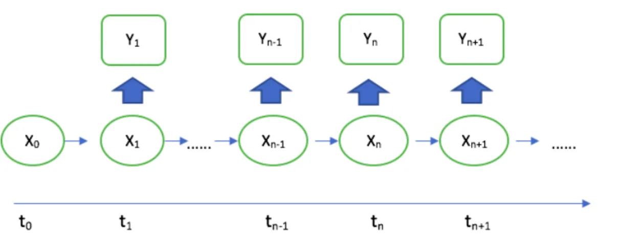
Now consider a time series of observations{Y1:n:Y1, ..., Yn}, consisting of n
obser-vations made at times t1, ..., tn, and let {X1:n : X1, ..., Xn} denote the state process.
1.2 Nonlinear State Space Models 3 statistical behavior of this hidden process is determined by the density hXn|Xn−1 and
the initial density hX0. On the other hand, the measurement process is modeled by
the density hYn|Xn.
Figure 1.1: State Space Models Schematic
The whole processes can be depicted as the above Figure 1.1, which shows the dependence among model variables. Under the Markovian assumption, the model can be simply expressed as the follows, for all n,
Xn|Xn−1 ∼hXn|Xn−1,
Yn|Xn∼hYn|Xn.
Because of the Markovian property of the process and the relationship between
X1:n and Y1:n, we know that for the state process, hXn|X0:n−1,Y1:n−1 =hXn|Xn−1.
hYn|X0:n,Y1:n−1 = hYn|Xn. Let θ be a p−dimensional real-valued parameter, θ ∈ R
p.
The state space structure implies that the joint density is determined by the ini-tial density, hX0(x0;θ), together with the conditional transition probability density,
hXi|Xi−1(xi|xi−1;θ), and the measurement density,hYi|Xi(yi|xi;θ), for i= 1,· · · , n. In
particular, we have hX0:n,Y1:n(x0:n, y1:n;θ) =hX0(x0;θ) n Y i=1 hXi|Xi−1(xi|xi−1;θ)hYi|Xi(yi|xi;θ)
This kind of nonlinear stochastic dynamical systems is widely used to model real data. In this case, the well known Kalman filter method may not be suitable for the statistical inference because of its assumptions. Instead, alternative mathematical procedures to analyze these nonlinear state space models have been proposed. In this context, many procedures have been proposed in recent years, leading to a prosperous atmosphere in the research of nonlinear state space models. In this thesis, we focus on the inference methods for nonlinear state space models. We present the estima-tion procedures and their algorithms including, iterated filtering (IF), approximate Bayesian computation (ABC) and particle Markov chain Monte Carlo (PMCMC).
1.3 Some Review of Literature 5
1.3
Some Review of Literature
Over the past decade, various researchers have made significant contributions to-wards the development of methodologies for statistical inference for state space models (Shumway and Stoffer 2006), i.e, partially observed Markov process models (Ionides et al. 2006; Bret´o et al. 2009). Sequential Monte Carlo, also known as particle filter (Doucet et al. 2001; Arulampalam et al. 2002; Capp´e et al. 2007) provides a standard method to obtain the log likelihood for this kind of stochastic dynamic models. Bret´o et al. (2009), He et al. (2010) introduced procedures whose main feature is that the full density does not need to be explicitly evaluated and only a simulator is required for the state space model.
Generally speaking, approaches that work with the full likelihood function are called full-information methods. On the other hand, approaches not based on the full likelihood are called feature-based procedures. Each method may be categorized as full-information or feature-based, Bayesian or frequentist. Both Bayesian (Liu and West 2001; Toni et al. 2009) and frequentist (Ionides et al. 2006; Poyiadjis et al. 2006) approaches to simulation likelihood-based inference via sequential Monte Carlo have been proposed. The maximum likelihood approach of Ionides et al. (2006, 2010) offers a possibility to carry on inference for general nonlinear stochastic state space
models.
1.4
Organization of Thesis
In this thesis, we focus on the inferential procedures and algorithms for nonlinear dynamic state space models. We evaluate the performance of these methods through simulation studies. Also, we conduct a case study applying nonlinear state space models to the analysis of time series data of annual forest fire counts in Canada.
The structure of this thesis is organized as follows. In Chapter 2, we present four algorithms for the statistical inference of nonlinear state space models. The first algo-rithm is intended to evaluate the likelihood, the other three are parameter estimation procedures. Chapter 3 constructs a nonlinear state space model and explores the performance of the discussed methods through simulation studies. Chapter 4 illus-trates the implementation of the model by analyzing the annual numbers of forest fires through Canada as an application. Finally, summary of the entire research and some future work is discussed in Chapter 5.
Chapter 2
Methodologies and Algorithms for
Nonlinear State Space Models
Statistical inference for state space models has been an active area of research. Yet, substantial restrictions or strict hypotheses upon the form of models have to be placed in advance when it comes to most existing inference methods. In nonlin-ear, non-Gaussian situations, some methods such as the Extended Kalman filter or the Gaussian sum filter are proposed to approximate the estimation for filtering and smoothing problems. However, the accuracy of these approximation, in most situ-ations, may be an issue. Sequential Monte Carlo (SMC) methods have emerged as the most popular and successful alternative to the Kalman filter extensions. Many
variations and elaborations to SMC have been proposed. Below, we will discuss four procedures and their respective algorithms that can be used for estimation, predic-tion and forecasting. These procedures are sequential Monte Carlo (also known as particle filter), iterated filtering (IF), particle Markov chain Monte Carlo (PMCMC), and approximate Bayesian computation (ABC).
2.1
Sequential Monte Carlo (Particle Filter)
Sequential Monte Carlo (SMC) methods, also known as particle filter, have far-reaching and powerful applications in modern time series analysis problems involv-ing state space models. Particularly, they are able to handle those nonlinear, non-Gaussian state space models, since particle filters algorithms do not rely on local linearization techniques or functional approximations. Instead, they are based on a set of simulations, which provides a convenient and attractive approach to computing the posterior distributions.
In the model we discussed in Section 1.2, we have that Xn|Xn−1 ∼ hXn|Xn−1 and
Yn|Xn ∼hYn|Xn. Consider the parameter valueθ ∈Θ and define Xn|(Xn−1 =x)∼hXn|Xn−1 ≡fθ(·|x)
2.1 Sequential Monte Carlo (Particle Filter) 9 where fθ(·|x) is the transition probability density for some static parameter θ and
gθ(·|x) is the marginal density probability. For the state process {Xn;n ≥ 1}, the
initial density is X1 ∼πθ(·).
The goal is to perform Bayesian inference conditional on the observations {y1:N =
(y1,· · · , yN)} for N ≥ 1. When θ ∈ Θ is a known parameter, the posterior density
πθ(x1:N|y1:N) is proportional to πθ(x1:N, y1:N). That is πθ(x1:N|y1:N)∝ πθ(x1:N, y1:N) where πθ(x1:N, y1:N) = πθ(x1)gθ(y1|x1) N Y n=2 fθ(xn|xn−1)gθ(yn|xn).
If θ ∈ Θ is unknown, we denote π(θ) as the prior density of θ. Then, the posterior density is proportional to the joint density
π(θ, x1:N|y1:N)∝πθ(x1:N, y1:N)π(θ).
The difficulty of statistical inference for nonlinear, non-Gaussian state space mod-els is that the densitiesπθ(x1:N, y1:N) andπ(θ, x1:N|y1:N) generally do not have a closed
form expressions. Therefore, these densities need to be approximated or evaluated numerically.
Now we can factorize the likelihood in the following way:
L(θ) =πθ(y1:N) = N Y n=1 πθ(yn|y1:n−1) (2.1)
Noted that πθ(yn|y1:n−1) = Z xn πθ(yn, xn|y1:n−1)dxn = Z xn πθ(xn|y1:n−1)πθ(yn|xn, y1:n−1)dxn = Z xn πθ(xn|y1:n−1)πθ(yn|xn)dxn, (2.2) we have L(θ) = N Y n=1 Z πθ(xn|y1:n−1)πθ(yn|xn)dxn.
Moreover, we can obtain the prediction formula using the Markovian property as
πθ(xn|y1:n−1) = Z xn−1 πθ(xn, xn−1|y1:n−1)dxn−1 = Z xn−1 πθ(xn−1|y1:n−1)πθ(xn|xn−1, y1:n−1)dxn−1 = Z xn−1 πθ(xn−1|y1:n−1)πθ(xn|xn−1)dxn−1 (2.3)
The filtering formula can be obtained by using the Bayes’ theorem as
πθ(xn|y1:n) = πθ(xn|yn, y1:n−1) = πθ(yn|xn, y1:n−1)πθ(xn|y1:n−1) πθ(yn|y1:n−1) = R πθ(xn|y1:n−1)πθ(yn|xn) xnπθ(xn|y1:n−1)πθ(yn|xn)dxn . (2.4)
Overall, the prediction and filtering formulas give us a recursion. Specifically, the prediction formula gives the prediction distribution at time n using the filtering
2.1 Sequential Monte Carlo (Particle Filter) 11 distribution at timen−1, and the filtering formula gives the filtering distribution at time n using the prediction distribution at time n, for all n= 1,2,· · · , N.
Now denote XF
n−1,j, j = 1, . . . , J as a set of J points drawn from the filtering
distributionπθ(xn−1|y1:n−1) at timen−1 andXn,jP as points drawn from the prediction
distribution πθ(xn|y1:n−1) at time n by simply simulating the process model: Xn,jP ∼
πθ xn|XnF−1,j
for j in 1 :J. Having obtainedXP
n,j, we can get a sample of points from the filtering distribution
πθ(xn|y1:n) at time n by resampling from
Xn,jP , j ∈ 1 : J with weights wn,j =
πθ yn|Xn,jP
. In addition, the Monte Carlo methods provide us an approximation to the conditional likelihood that we obtained from the above. That is
Ln(θ) = πθ(yn|y1:n−1) = Z xn πθ(xn|y1:n−1)πθ(yn|xn)dxn, (2.5) can be estimated by ˆ Ln(θ)≈ N1 Pjπθ(yn|Xn,jP ), wherever XP
n,j is random sample drawn from πθ(xn|y1:n−1).
Now we can iterate this procedure through the data, one step at a time, alternately simulating and resampling, until we reach n = N. Then the full log likelihood has
approximation: `(θ) = logL(θ) =X n logLn(θ) ≈X n log ˆLn(θ). (2.6)
In general, there is a more generic way to express the whole calculation procedure of particle filter (Andrieu et al. 2010). We aim to yield the estimate, ˆπ. The procedure can be summarized in the following steps.
Particle Filter Algorithm
Step 1. At time t = 1, define an importance density v(·) for importance sampling; we aim to approximate πθ(x1|y1).
a. Draw a sample of J particles Xk
1 = (X11,· · · , X1J) from vθ(x1|y1).
b. Calculate the normalized importance weights and denote them as Wk
1 = (W1 1,· · · , W1J), where w1(X1k) = πθ(X1k, y1) vθ(X1k|y1) W1k = w1(X k 1) PJ m=1w1(X1m) .
2.1 Sequential Monte Carlo (Particle Filter) 13 c. The estimate of πθ(x1|y1) can be calculated by
ˆ πθ(x1|y1) = J X k=1 W1kδXk 1(x1)
whereδx(·) is the Dirac Delta function.
d. Use these particles and weights to resample J new particles from the ap-proximation, ˆπθ(x1|y1).
Step 2. Iteration. At time t = 2,3,· · · , N −1, we again use importance sampling to approximateπθ(x1:t|y1:t).
a. DenoteAk
t−1 as the index of the parent of particlesX1:ktat timet−1; draw
a sample Ak
t−1 ∼ M(·|Wt−1), where Wt = (Wt1,· · · , WtJ) and M(·|p) is
the multinomial distribution with parameterp. b. Draw a sample Xk t ∼v ·|yt, X Ak t−1 t−1 , and set Xk 1:t= XA k t−1 1:(t−1), X k t . c. Calculate the normalized importance weights:
wt(X1:kt) = πθ(X1:kt, y1:t) πθ XA k t−1 1:(t−1), y1:(t−1) vθ Xk t|yt, X Ak t−1 t−1 Wtk = wt(X k 1:t) PJ m=1wt(X1:mt) .
given by ˆ πθ(x1:t|y1:t) = J X k=1 WtkδXk 1:t(x1:t)
whereδx(·) is the Dirac Delta function.
Step 3. At time t =N, the procedure yields the approximation of the posterior density
πθ(x1:N|y1:N) given by ˆ πθ(x1:N|y1:N) = J X k=1 WNkδXk 1:N(x1:N).
At the end, the estimate of the likelihoodπθ(y1:N) is
ˆ πθ(y1:N) = ˆπθ(y1) N Y t=2 ˆ πθ(yt|y1:(t−1)) where ˆ πθ(yt|y1:(t−1)) = 1 N J X k=1 wt(X1:kt).
2.2 Iterated Filtering 15
2.2
Iterated Filtering
Iterated filtering technique is a significant inference method that can maximize the likelihood obtained by SMC (Ionides et al. 2006, 2011). It’s specially practical to the state space models. The idea of iterated filtering is that an optimization can be obtained by taking parameter perturbations into consideration when iteratively reconstructing the latent states. In terms of the unknown parameter space, stochastic perturbations are introduced into the method, which can be dynamically used to search for a suitable parameter estimate.
The main goal of the algorithm is to find the maximum likelihood estimates of the unknown parameters. As long as a proper procedure iterates with successively diminished perturbations, the estimating result will converge to the maximum like-lihood estimate. Ionides et al (2015) improve the iterated filtering algorithm based on the convergence of an iterated Bayes map, and name the algorithm as IF2. In general, the IF2 algorithm can be summarized as the following procedure.
Iterated Filtering Algorithm
Step 1. Initialization. Arbitrary starting parameter [θj]0, where j = 1,2,· · ·J with J
wherem= 1,2,· · · , M withM as the number of operation. Let the superscript
F represent filtering recursion andP represent prediction recursion.
Step 2. Iteration. For m= 1,2,· · · , M,
1. Draw a random sample of parameter, [θF
0,j]m ∼γ0(θ|[θj]m−1;σm).
2. Draw a random sample of states [XF
0,j]m ∼fX0(x0; [θ F
0,j]m).
3. Iteration. Forn = 1,2,· · · , N, a. Draw a random sample [θP
n,j]m ∼γn(θ|[θFn−1,j]m;σm).
b. Draw a random sample [XP
n,j]m ∼π(xn|[XnF−1,j]m; [θjP]m).
c. Calculate weights: [wn,j]m =π(yn|[Xn,jP ]m; [θPn,j]m).
d. Draw indices k1:J with P{kj =s}= [wn,s]m/PJu=1[wn,u]m.
e. Let [θFn,j]m = [θn,kP j]m and [X
F
n,j]m = [Xn,kP j]m.
4. Set [θj]m = [θFN,j]m.
2.3 Particle Markov Chain Monte Carlo (PMCMC) 17
2.3
Particle Markov Chain Monte Carlo (PMCMC)
Particle Markov chain Monte Carlo (PMCMC) is a Bayesian inference method us-ing full information. It’s proposed by Andrieu et al. (2010) to perform inference on the unknown parameter vector θ. It targets the full joint posterior distribution
π(θ, x1:N|y1:N). PMCMC methods combine likelihood evaluation via particle filter
with MCMC moves in the parameter space. It works well in nonlinear non-Gaussian scenarios while the traditional MCMC methods can fail in this specific situation. One common used PMCMC algorithm is termed as particle marginal Metropolis-Hastings (PMMH). It plugs the unbiased likelihood estimate obtained by particle filter into the Metropolis-Hastings update procedure to get the desired posterior distribution for the parameters (Andrieu and Roberts 2009).
First we take a brief review of the Metropolis-Hastings algorithm, which is one of the most common MCMC algorithms. It can generate correlated variables from a Markov chain. Given the target densityπ(x1:N, y1:N), it is associated with a proposed
density v(·|x).
So the MH algorithm can be summarized as below. Given a target density π(x) and a proposal densityv(·|x), a new Markov chain{Xm∗}whose stationary distribution is π(x) can be generated by the following algorithm:
Metropolis-Hastings Algorithm
Step 1. Start with an arbitrary x∗0, generatex0 fromv(·|x∗m−1). Step 2. Compute the probability ρ(x∗m,x0) = minn1, π(x
0 )v(x∗m|x 0 ) π(x∗ m)v(x 0| x∗ m) o .
Step 3. Set x∗m+1 = x0 with probability ρ(x∗m,x0); set x∗m+1 = x∗m with probability 1−ρ(x∗m,x0).
In our state space models, when the parameter θ is unknown, we are interested in sampling from π(θ, x1:N|y1:N). The PMMH algorithm will focus on jointly updating
θ and x1:N. Given that π(θ, x1:N|y1:N) = π(θ|y1:N)πθ(x1:N|y1:N), a natural choice of
proposal density for an MH update is
v(θ∗, x∗1:N|θ, x1:N) = v(θ∗|θ)πθ∗(x1:∗N|y1:N). (2.7) So the resulting MH acceptance ratio is given by
A= π(θ ∗, x∗ 1:N|y1:N)v(θ, x1:N|θ∗, x∗1:N) π(θ, x1:N|y1:N)v(θ∗, x∗1:N|θ, x1:N) = πθ∗(y1:N)π(θ ∗)v(θ|θ∗) πθ(y1:N)π(θ)v(θ∗|θ) . (2.8)
2.3 Particle Markov Chain Monte Carlo (PMCMC) 19 The PMMH algorithm can be summarized as the following procedure.
PMMH Algorithm
Step 1. Initialization. Arbitrary starting parameter θ0; run the SMC algorithm with
J particles targeting πθ0(x1:N|y1:N) to obtain the estimates ˆπθ0(·|y1:N) and the
marginal likelihood estimate ˆπθ0(y1:N); draw a random sampleX
0
1:N ∼πˆθ0(·|y1:N).
Step 2. Iteration. Denote M as the number of operation. For m= 1,2,· · · , M, 1. Draw a parameter θP from the proposal distribution θP ∼v(·|θm−1).
2. Run the SMC algorithm with J particles targeting πθP(x1:N|y1:N) to
ob-tain the density estimate ˆπθP(·|y1:N) and the marginal likelihood estimate
ˆ
πθP(y1:N); draw a random sample X1:PN ∼πˆθP(·|y1:N).
3. Calculate the probability ρm = min n
1, πθP(y1:N)π(θP)v(θm−1|θP) πθm−1(y1:N)π(θm−1)v(θP|θm−1)
o
.
4. With probability ρm, set θm = θP, X1:mN = X1:PN, ˆπθm(y1:N) = ˆπθP(y1:N);
otherwise, setθm =θm−1, X1:mN =X m−1
1:N , ˆπθm(y1:N) = ˆπθm−1(y1:N).
Step 3. After M times iterations, we will have the samples θ1:M where the posterior
2.4
Approximate Bayesian Computation (ABC)
ABC algorithms are Bayesian feature-based methods to evaluate the posterior dis-tributions through simulations instead of calculations of likelihood functions. They compare the distance between the observed and simulated data (Pritchard et al. 1999; Marjoram et al. 2003; Sisson et al. 2007).
Let θ as the parameter vector we are about to estimate in our models. Denote
π(θ) as its prior distribution and x0 as the observed data. Our goal is to obtain an
approximation of the posterior distribution, π(θ|x0). According to Bayes’ Theorem,
we haveπ(θ|x0)∝f(x0|θ)π(θ), wheref(x0|θ) is the likelihood ofθ given the observed
data x0.
A simple ABC algorithm is called the rejection sampler (Pritchard et al. 1999). It includes the following steps:
Rejection Sampler Algorithm
Step 1. Sample a candidate parameter θ∗ from a the prior distribution π(θ).
Step 2. Simulate a dataset x∗ fromf(x|θ∗).
2.4 Approximate Bayesian Computation (ABC) 21 using a distance functionD; and a tolerance, ifD(x0, x∗)≤, then acceptθ∗,
otherwise reject.
Step 4. Repeat the above steps until one has a sample {θ∗k} of size M where infer-ence about π(θ|x) can be done by taking uniform weights Wk = 1
M for k =
1,2, . . . , M.
Often times, instead of using the full data set to obtain the posterior distribution, either because we only have summary statistics or because of the dimension of the data, we would like to obtain the distribution of the parameters given a set of summary statistics. For this situation, we define a distance function based on the summary statistics. These summary statistics are the features of the full dataset. The features, also called probes (Kendall et al. 1999), are denoted by a collection of functions,
S = (S1,· · · ,Sd), where each Si maps an observed time series to a real number. We
write S = (S1,· · · , Sd) for the vector-valued random variable withS =S(Y1:N), with
hS(s;θ) being the corresponding joint density. Also, the observed feature vector is s0
wheres0i =Si(y1:N). The goal of ABC is to estimate the posterior distribution of the
unknown parameters given S = s0. Denote the distance function as ρ and s as the
But the acceptance rate of this ABC rejection sampler will be quite low if the prior distribution vastly differs from the posterior distribution. To solve the problem, Marjoram et al. (2003) proposed an ABC method based on Markov chain Monte Carlo. The procedure can be summarized as below:
ABC Algorithm
Step 1. Initialization. Arbitrary starting parameter θ0.
Step 2. Iteration. Denote M as the number of operation. For m= 1,2,· · · , M, 1. Draw a proposed parameterθP from a proposal distributionθP ∼v(·|θ
m−1).
2. Sample a dataset xP fromf(x|θP).
3. Compute observed probes s0 and the simulated probes sP.
4. Calculate the probability pm = min n
1, π(θP)v(θm−1|θP)
π(θm−1)v(θP|θm−1)I[ρ(s0,sP)≤] o
. 4. With probability pm, set θm =θP; otherwise, set θm =θm−1.
Step 3. After M times iterations, we obtain the samples θ1:M, as well as the posterior
2.5 The R Package: POMP 23
2.5
The R Package: POMP
The R package POMP (King et al. 2016) provides a suite of tools for analysis of time series data based on state space models. It provides a very flexible framework for statistical inference using nonlinear, non-Gaussian state space models. Many modern statistical methods have been implemented in this framework including sequential Monte Carlo, iterated filtering, particle Markov chain Monte Carlo, approximate Bayesian computation, maximum synthetic likelihood estimation, etc.
POMP is fully object-oriented. A partially observed Markov process model is represented by an object of class ’pomp’. Methods for the class ’pomp’ use vari-ous components to carry out computations on the model. A brief summary of the mathematical notations corresponding to the elementary methods is shown as below:
Table 2.1: A Brief Summary of notations for POMP Models Method Mathematical terminology
rprocess Simulate from hXn|Xn−1(xn|xn−1;θ)
dprocess Evaluate hXn|Xn−1(xn|xn−1;θ)
rmeasure Simulate from hYn|Xn(yn|xn;θ)
dmeasure Evaluate hYn|Xn(yn|xn;θ)
rprior Simulate from the prior distribution π(θ)
dprior Evaluate the prior densityπ(θ)
init.state Simulate from hX0(x0;θ)
timezero Initial time t0
time Timest1:N
obs Datay1:N
states Statesx0:N
There are many examples illustrated in the package, as well as a large vol-ume of corresponding R and C codes that are provided with the package. Further documentation and an introductory tutorial can be found on the POMP website, http://kingaa.github.io/pomp.
Chapter 3
Simulation Study
Nonlinear state space models can be used to analyze the time series of count data. One of the applications is to model the number of major (with magnitude 7 or higher on the Richter scale) earthquakes each year. We use the model from Langrock (2011) and Zeger (1988), which assumes that the number of earthquakes yt is a conditional
Poisson distributed variable with mean λt. Also, we assume that the mean of λt
follows an AR(1) process,
log(λt)−µ=φ(logλt−1−µ) +σvt
wherevtdenotes a standard Gaussian random variable. By introducingxt=log(λt)−
xt+1|xt ∼ N(φxt, σ2)
yt|xt∼ P(βext)
where the parameter vector isθ ={β, σ, φ}with the constraintsφ ∈(−1,1)⊂Rand
{σ, β} ∈ R2
+. Here, P(λ) denotes a Poisson distributed variable with mean λ. That
is, the probability ofk ∈Nearthquakes during yeart is given by the probability mass function (PMF),
P{Yt=k}=e−λ
λk k!
In this chapter we set up a nonlinear state space model and present the simulation study of a time series of count data to compare the four methodologies we have studied: SMC, IF, PMCMC, and ABC.
3.1
Simulation Setup
We use R software to generate the random numbers. Set the parameter vector θ as
θ = {β = 1, σ = 0.1, φ = 0.2} and the initial state as x0 = 1. It leads to the state
process,
xt+1|xt∼ N(0.2xt,0.12)
3.1 Simulation Setup 27
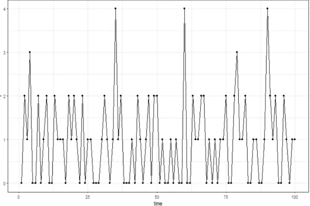
yt|xt∼ P(ext).
We simulate a time period from 1 to 100, and the nonlinear state space model generate a series of simulated counts. The plot of simulated counts is shown in Figure 3.1. Since the true value of parameters we set up are small, the largest simulated outcomes are just 4 and there are lots of zero in this simulation.
3.2
Simulation Analysis
Based on the series of count data we simulated, we can use the iterated filtering approach to obtain the maximum likelihood estimate of parameters. In R, it can be used the function named mif in POMP package to obtain the results. Since the parameters in our model are constrained to be positive, we prefer to transform them into an unconstrained scale to estimate instead. So we designate the logarithm trans-formation to the parameters when estimating. In order to improve the computation efficiency, the foreachRpackage (Revolution Analytics and Weston 2014) will be used to parallelize the computations.
We run 10 trajectories, and for each run, the number of iterations is 100, the number of particles is 2000. The calculation result is shown in Figure 3.2. It shows that each trajectory converges to an estimate. For the parameter logσ and logφ, most of runs have different estimations after 100 iterations. But for logβ and the log-likelihood logL, nine of ten runs converges to a really close estimate. Usually, we will focus on the estimate with the highest estimated log-likelihood.
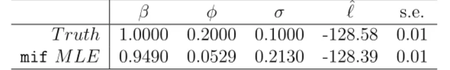
Specifically, we can take a comparison between the parameter estimates and their true values. From Table 3.1, we obtain the MLE of parameters as ˆθM LE = {β =
3.2Simulation Analysis 29 −1 55 −1 45 −1 35 −1 25 lo g L −1 .5 −0 .5 0. 5 lo gβ −3 .5 −2 .5 −1 .5 lo gσ 0 20 40 60 80 100 −3 .0 −2 .0 −1 .0 0. 0 mifiteration lo gφ
MLE is -128.39, and its standard error is 0.01.
Table 3.1: Results of Estimating Parameters Using IF2 Algorithm
β φ σ `ˆ s.e.
T ruth 1.0000 0.2000 0.1000 -128.58 0.01
mifM LE 0.9490 0.0529 0.2130 -128.39 0.01
For the iterated filtering method, we can consider two more cases with other true values as comparison. In Case Two, we set θ2 = {β = 5, σ = 0.3, φ = 0.5}, and the
MLE obtained by the iterated filtering is ˆθ2M LE = {β = 4.97, σ = 0.372, φ = 0.47}
with the log-likelihood -253.91. The result is shown in Table 3.2.
Table 3.2: Results of Estimating Parameters Using IF2 Algorithm in Case Two
β φ σ `ˆ s.e.
T ruth 5.0000 0.5000 0.3000 -254.61 0.05
mif M LE 4.9700 0.4700 0.3720 -253.91 0.13
Likewise, we set the true values of θ in Case Three as θ3 ={β = 10, σ = 0.5, φ=
0.7}. Correspondingly, we can obtain the MLE as ˆθ3M LE = {β = 6, σ = 0.488, φ =
0.61}. The detailed result is shown in Table 3.3.
Table 3.3: Results of Estimating Parameters Using IF2 Algorithm in Case Three
β φ σ `ˆ s.e.
T ruth 10.0000 0.7000 0.5000 -291.38 0.09
mif M LE 6.0000 0.6100 0.4880 -288.00 0.19
The above shows that the mifprocedure can successfully maximize the likelihood and propose a reasonable parameter estimate.
3.2 Simulation Analysis 31 In the following methods, we just consider the original values of θ, which is θ =
{β = 1, σ = 0.1, φ= 0.2}. Now the statistical estimation for the unknown parameters can be carried out by using PMCMC algorithm that we’ve discussed in Section 2.3. PMCMC is a full-information Bayesian method that it pays large price to run the SMC algorithm to finally obtain the Metropolis-Hastings acceptance probability. Using the R function pmcmc in POMP package, we specify a uniform prior distribution on unknown parameters and set the particles number as 100. We run 5 independent MCMC chains with 30,000 iterations for each chain. After a mass of calculation, we can obtain a swam of the posterior parameter estimates.
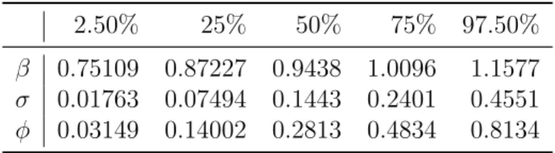
Table 3.4: PMCMC Quantiles for Each Parameter 2.50% 25% 50% 75% 97.50%
β 0.75109 0.87227 0.9438 1.0096 1.1577
σ 0.01763 0.07494 0.1443 0.2401 0.4551
φ 0.03149 0.14002 0.2813 0.4834 0.8134
Table 3.4 shows the PMCMC quantiles for each parameters, and we use the 50% quantile as the estimates of unknown parameters. So we can obtain ˆθP M CM C ={β =
0.9438, σ= 0.1443, φ= 0.2813}.
Besides, we can calculate the mean and the standard deviation of paramters β, σ, and φ. As the Bayesian inference, we can also calculate their naive standard errors and the time-series standard error from the big volume of posterior parameter sample
set.
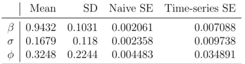
Table 3.5: PMCMC Empirical Mean and Standard Deviation for Each Parameter, Plus Standard Error of the Mean
Mean SD Naive SE Time-series SE
β 0.9432 0.1031 0.002061 0.007088
σ 0.1679 0.118 0.002358 0.009738
φ 0.3248 0.2244 0.004483 0.034891
Table 3.5 reflects the PMCMC empirical mean and standard deviation for each parameter, as well as the standard error of the mean. As we know, the true value of
β is 1, while the mean of the posterior distribution of β is 0.9432 and its standard deviation is 0.1031.
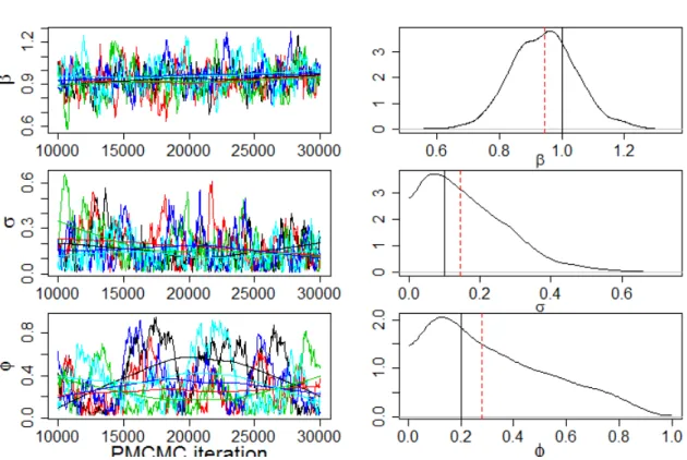
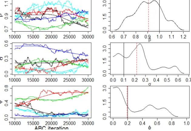
The diagnostic plots for the PMCMC algorithm is shown in Figure 3.3. The trace plots in the left column show the evolution of 5 independent MCMC chains from iterations 10001 to 30001. We can see that for β and σ, the five traces are relatively close, while the traces of φ are very different. In addition, based on the big swam of posterior estimates, we can also plot the kernel density estimates of the marginal posterior distributions, which are shown at right. Specifically, the solid vertical line is the true parameters and the red dashed line is the PMCMC estimates of parameters.
3.2 Simulation Analysis 33
As comparison, we apply the ABC algorithm to obtain the evaluation of unknown parameters. Since the ABC algorithm use partial features of the data, we need to designate the probes first. We set up the mean and their autocorrelation function as their probes. In Section 2.4, we’ve discussed the procedures. Now using the R
function abc in POMP package, we can obtain the posterior parameter estimates based on partial feature of data. Also, we run 5 independent chains and for each one the iteration step is 30,000.
Table 3.6: ABC Quantiles for Each Parameter 2.50% 25% 50% 75% 97.50%
β 0.69828 0.82642 0.9063 0.9838 1.1181
σ 0.01692 0.11229 0.2172 0.2828 0.5765
φ 0.02464 0.07618 0.1918 0.5072 0.736
Table 3.6 shows the ABC quantiles for each parameters, and we use the 50% quantile as the estimates of unknown parameters. So we can obtain ˆθABC = {β =
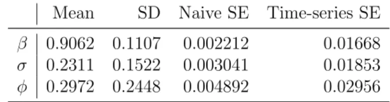
0.9063, σ = 0.2172, φ = 0.1918}. Table 3.7 reflects the ABC empirical mean and standard deviation for each parameter, as well as the standard error of the mean. Table 3.7: ABC Empirical Mean and Standard Deviation for Each Parameter, Plus Standard Error of the Mean
Mean SD Naive SE Time-series SE
β 0.9062 0.1107 0.002212 0.01668
σ 0.2311 0.1522 0.003041 0.01853
3.2 Simulation Analysis 35 In addition, the diagnostic plots for the ABC algorithm is shown in Figure 3.4. We can see that the five chains diverge in different directions, which means the model is quite sensitive to the parameters. Kernel density estimates of the marginal posterior distributions are shown at right. These posterior distribution are plot by the posterior parameter estimates that obtained by ABC algorithm usingR. The solid vertical line is the true parameters and the red dashed line is the ABC estimates of parameters.
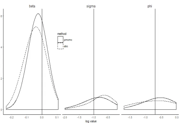
Figure 3.5: The Marginal Posterior Distributions of log10 Value of Parameters
In the end, we compare the statistical efficiency between ABC and PMCMC. We take the log10 value for all the posterior parameter estimates obtained by PMCMC and ABC. Then We plot their density functions into the same figure.
Figure 3.5 shows the marginal posterior distributions using full information via PMCMC (solid line) and partial information via ABC (dashed line). Kernel density estimates are illustrated for the posterior marginal densities of log10(β), log10(σ), and log10(φ), respectively. It reflects that ABC leads to somewhat broader posterior
3.2 Simulation Analysis 37 distributions than the posteriors from PMCMC. In some ways, the reason may be straightforward. Since PMCMC use more information of the data than that of ABC, PMCMC then should have a more narrow and precise estimate than ABC.
Application: The Analysis of
Annual Forest Fire Counts in
Canada
4.1
Background
Forest fire is a major environmental problem in Canada. It can cause catastrophic damages on natural resources and bring serious economic and social impacts. Each year, there are over thousands of forest fires around Canada, causing the destruction of large volumes of forest land. Nevertheless, forest fires have also benefits for the
4.2 Data Description 39 health of the flora. For example, forest fires have been associated to the control of spread of beatle trees. According to the statistics from the Natural Resources Canada, about 7,588 forest fires have occurred each year over the last 25 years. Therefore, it is necessary to maintain an efficient wildland fire management in order to predict and manage risks and benefits.
A comprehensive study of forest fire activity would require the analysis of annual number of forest fires. Often a Poisson model has been employed for the number of fires, see Dayananda (1977), Mandallaz and Ye (1997). In this work, we consider the historical recorded data of forest fires as a time series of count data. We propose a nonlinear state space model to analyze the annual number of forest fires in Canada. And the statistical inference and estimation for the proposed model is then processed by the four methodologies that we have discussed in Chapter 2.
4.2
Data Description
The data we analyze consist of yearly total number of forest fires occurred in Canada from 1970 to 2014. This time series of forest fire counts is collected from the National Forestry Database (http://nfdp.ccfm.org/dynamic report/dynamic report ui e.php). We select the reporting agency as Canada, and the reporting item is the number of
fires in total. This dataset reflects the overall forest fire occurrences in Canada for each year. Table 4.1 shows the collected data.
Table 4.1: Total Number of Forest Fires Year Total Fires Year Total Fires
1970 9250 1993 6043 1971 9167 1994 9763 1972 8232 1995 8486 1973 7593 1996 6349 1974 8129 1997 6148 1975 11178 1998 10723 1976 10236 1999 7633 1977 8945 2000 5349 1978 8028 2001 7753 1979 10051 2002 7861 1980 9138 2003 8230 1981 10095 2004 6680 1982 8942 2005 7542 1983 8935 2006 9820 1984 9220 2007 6917 1985 9354 2008 6278 1986 7320 2009 7210 1987 11301 2010 7291 1988 10741 2011 4743 1989 12185 2012 7956 1990 10111 2013 6264 1991 10327 2014 5152 1992 9068
4.2 Data Description 41
Figure 4.1: The Trend Plot of the Total Number of Forest Fires
The trend plot of this time series of forest fire counts can be illustrated in Figure 4.1 as above. We can see that in the recent 45 years, the minimum annual number of forest fires is 4,743, while the maximum number is 12,185. The general tendency of forest fires is declining though it oscillates each year.
Also, we can plot the histogram of forest fires counts, as shown in Figure 4.2. This figure shows that the distribution of the historical fires data is slightly left-skewed, with an average of 8,394 yearly occurrences.
4.3 Model Setup 43
4.3
Model Setup
Now we propose a nonlinear state space model to practically simulate and replicate the real counts generating process of the forest fires. First of all, we consider the state process. Assuming it is a discrete time process model, let’s denote{Nt, t = 0,1,2,· · · }
as the state space. Then the state process can be set as below:
Nt+1 =
rNt
1 + Nt
K
t, t∼ LN(−12σ2, σ2),
where the unknown parameter vector is θ = {r, K, σ} and t follow a log-normal
distribution. This stochastic model is known as the Beverton-Holt model, which was introduced in the context of fisheries by Beverton & Holt (1957) . Despite it is a classic discrete time population model usually applied in ecology or epidemiology, it might still be able to depict the potential relationships between those transferable state spaces as a latent state system for the annual count of forest fires. Herercan be explained as the inherent growth rate, andK is assumed as a quasi-carrying capacity. We can define the state Nt as the true population size of forest fire counts at Year t.
For the measurement process, let us assume that the observation at time tfollows a Poisson distribution with a parameter size Nt. That leads to the annual observed
number of forest firesyt follows:
4.4
Model Simulation
For those state spaces, we established the implied state-generating structure, but the parameter vector still remains unknown. The difficulties are how to estimate the latent unknown parameters. According to our observed numbers of forest fire, we can try a reasonable initial guess for the parameter vector θ = {r, K, σ}, and plot the simulated states.
Let us assume the initial parameters are θ0 = {r = 1.4, K = 20000, σ = 0.15},
and the initial state value is N0 = 8000. With the process model in place, we can
simulate the state spaces and plot 10 state realizations with the initial parameters. It is shown in Figure 4.3. Since the measurement model we are considering follows a Poisson distribution with parameterNt, it also reflects the simulated annual averages
4.4 Model Simulation 45
Figure 4.3: 10 Simulated State Realizations Based on the Process Model with the Initial Parameters
Figure 4.4: A Comparison Between Simulated State Realizations and Simulated Ob-servation Realizations
With the measurement model, we can now simulate for the full nonlinear state space model. The result is shown in Figure 4.4. It is a comparison between the simulated states and the corresponding simulated observations. From the Figure 4.4, we find those trajectories are similar, which is quite straightforward. Another plot that shows the relationship between latent states and observed measurements is illustrated in Figure 4.5. All the points almost fall into a line, which reveals a property of the Poisson distribution in some ways.
4.4 Model Simulation 47
Figure 4.6: 10 Simulated Count Trajectories Based on Initial Parameters and the Actual Observed Number of Fires
To sum up, based on the nonlinear state space model that we have set up as well as the initial parameters that we have assigned, we can simulate the fitted model and compare it against the observed data - the total number of forest fires occurred in Canada. Figure 4.6 shows that our simulated trajectories cover the real data trajectory, and it exists certain similar shape. That means the initial parameters we assigned are plausible and the fitted model looks feasible and practical.
4.5 Model Estimation 49
4.5
Model Estimation
Given the initial parameters, we can evaluate the likelihood of the forest fires data using the particle filter. Since the larger number of particles we use, the smaller Monte Carlo error but the greater computational burden we have, we decide to run 1000 particles to estimate the log likelihood at the initial guess of parameters θ0 =
{r = 1.4, K = 20000, σ = 0.15}, and the initial state value is N0 = 8000. We can
obtain the log likelihood as -418.6927.
We will use the iterated filtering (Ionides et al. 2006, 2015) to obtain a maximum likelihood estimate for the real forest fires data. Since the parameters of the model
θ = {r, K, σ} are constrained to be positive, we transform them to a scale on which they are unconstrained when estimating.
Table 4.2: Results of Estimating Parameters
r K σ `ˆ s.e.
Initial Guess 1.40 20000 0.150 -384.21 0.31
mifM LE 1.29 27900 0.172 -383.74 0.63
We replicate the iterated filtering search, and make a careful estimation of the log likelihood ˆ` as well as its standard error at each of the resulting point estimates. And then the parameter vector corresponding to the highest likelihood is chosen as the numerical approximation to the maximum likelihood estimates of parameters. The
resulting estimates are shown in Table 4.2. We can see the estimating parameters of the nonlinear state space model by maximum likelihood using iterated filtering are ˆ
θM LE ={ˆr= 1.29,Kˆ = 27900,σˆ = 0.172}.
Figure 4.7: The Histogram of Log-likelihood at Different Parameter Values. Blue line represents the Maximum Likelihood Estimate, while pink line represents the initial guess.
We proceed to carry out 100 replicated particle filters at the initial guess and the MLE of parameters. A histogram shown as Figure 4.7 is plot to compare the calculated log likelihood at the two different points. We can see that the median
4.5 Model Estimation 51 of the log likelihoods at the MLE is -406.9707, which is greater than that of log likelihoods at the initial guess, -412.7548. It means that the MLE is better.
Now we carry out a local search of the likelihood surface using the IF2 Algorithm. Given a model and a set of data, the likelihood surface is well defined. We set the starting point asθstart={r= 1.1, K = 10000, σ= 0.05}and a fixed initial state value
8000. Also, we set a perturbation size of 0.02 and the cooling type as geometric. Then runningR codes, we can obtain the diagnostic plots shown as Figure 4.8.
K sigma X.0 loglik nfail r 0 10 20 30 40 50 0 10 20 30 40 50 0 10 20 30 40 50 1 2 3 7999.50 7999.75 8000.00 8000.25 0 10 20 30 0.1 0.2 −1500 −1200 −900 −600 5000 10000 15000 20000 iteration value
In addition, the Figure 4.9 illustrates the geometry of the likelihood surface in a neighborhood of the point estimate.
loglik 1.5 2.0 2.5 3.0 3.5 0.19 0.21 0.23 0.25 −403 −401 1.5 2.0 2.5 3.0 3.5 r K 5000 15000 −403 −402 −401 −400 0.19 0.21 0.23 0.25 5000 10000 15000 20000 sigma
Figure 4.9: A Local Search of the Likelihood Surface
We can also carry out a global search by trying all remotely sensible parameter vectors that are contained in a large box of parameter space. A starting values vector is randomly drawn from the box. Then the result of the global search is shown in Figure 4.10. The best result of this search had a log likelihood of -397.2959 with a standard error of 0.6764758. A scatterplot is used to visualize the global geometry
4.5 Model Estimation 53 of the likelihood surface. It is shown in Figure 4.11 that gray points are the starting values and red points are the IF2 estimates. We conclude that optimization attempts from various starting points converge on a particular region in parameter space.
Figure 4.10: A Global Search of the Likelihood Surface
To get an idea of what the likelihood surface looks like corresponding to the parameter r and K, we can evaluate the likelihood at a grid of points and visualize the surface directly. In particular, all points with log likelihoods less than 50 units below the maximum are shown in gray in Figure 4.12.
4.5 Model Estimation 55 10000 15000 20000 25000 30000 35000 0.5 1.0 1.5 2.0 r K −450 −440 −430 −420 −410 loglik
Now we specify a prior distribution on unknown parameters and carry out Bayesian inference. The PMCMC algorithm is applied to draw a sample from the posterior. Table 4.3 shows the PMCMC quantiles for each parameters, and we use the 50% quantile as the estimates of unknown parameters. So we can obtain ˆθP M CM C ={r=
1.298, K = 27943, σ = 0.174}. The diagnostic plots for the PMCMC algorithm is shown in Figure 4.13. The trace plots in the left column show the evolution of 5 independent MCMC chains from iterations 10001 to 30001. Kernel density estimates of the marginal posterior distributions are shown at right. The solid vertical line is the initial guess of parameters and the red dashed line is the PMCMC estimates of parameters.
Table 4.3: PMCMC Quantiles for Each Variable
2.50% 25% 50% 75% 97.50%
r 1.2430 1.2740 1.2980 1.3150 1.3460
σ 0.1386 0.1593 0.1740 0.1854 0.2162
4.5 Model Estimation 57
Also, we apply the ABC algorithm to obtain the evaluation of unknown param-eters. Table 4.4 shows the ABC quantiles for each parameters, and we use the 50% quantile as the estimates of unknown parameters. So we can obtain ˆθABC = {r =
1.397, K = 19050, σ= 0.1582}. The diagnostic plots for the ABC algorithm is shown in Figure 4.14. Kernel density estimates of the marginal posterior distributions are shown at right. The solid vertical line is the initial guess of parameters and the red dashed line is the ABC estimates of parameters.
Table 4.4: ABC Quantiles for Each Variable
2.50% 25% 50% 75% 97.50%
r 1.1980 1.3230 1.3970 1.4720 1.5660
σ 0.1175 0.1432 0.1582 0.1756 0.2046
4.5 Model Estimation 59
Summary and Future Work
In this thesis, we mainly proposed a nonlinear state space model to analyze the annual forest fires occurred in Canada. This proposed model is different from the traditional Poisson regression models or Logistic models that are usually applied in the fires occurrence analysis. It provides a flexibility and reliability to the analysis of the real forest fires dataset. The difficult part of the proposed model is the statistical inference and estimation for the unknown parameters. To solve the problems, we used four numerical methodologies and algorithms, which have been proved to be feasible and practical in the literature. They are particle filter (also named sequential Monte Carlo), iterated filtering (IF), particle Markov chain Monte Carlo (PMCMC), and approximate Bayesian computation (ABC), respectively. All these methods have
Summary and Future Work 61 plug-and-play property, which can be easily programmed and run in the R statistical software using the package POMP.
The paper first provides a brief introduction to the nonlinear state space model. Then, it takes a focus on the methodologies applied to fit the model and obtain the parameter estimates. Also, a simulation study is carried out to analyze a series of simulated counts using the methods. At the end, an analysis of the annual forest fires using the nonlinear state space model is presented. The unknown parameters of the model are estimated by using the proposed numerical methods with satisfactory outcomes.
For future work, we can add a parameter for the measurement process based on our original model. That means the new measurement process would be P(φNt). Of
course, an additional unknown parameter will bring larger computational costs to our analysis. Also, we may assume the measurement process follows a Negative Binomial distribution, considering the over-dispersion situation. Moreover, one may also be interested in the role of a vector-valued covariate process in explaining the forest fires data. Then modeling and inference conditional on covariates can be carried out in the further work as well.
[1] Andrieu C, Doucet A, Holenstein R (2010). Particle Markov Chain Monte Carlo Methods. Journal of the Royal Statistical Society B, 72(3), 269-342.
[2] Arulampalam MS, Maskell S, Gordon N & Clapp T (2002). A tutorial on particle filters for online nonlinear, non-Gaussian Bayesian tracking. IEEE Trans. Signal Process, 50, 174-188.
[3] Beaumont MA (2010). Approximate Bayesian Computation in Evolution and Ecology. Annual Review of Ecology, Evolution, and Systematics, 41, 379-406. [4] Bhadra A (2010). Discussion of Particle Markov Chain Monte Carlo Methods by
C. Andrieu, A. Doucet and R. Holenstein.Journal of the Royal Statistical Society B,72, 314-315.
[5] Bret´o C, He D, Ionides EL & King A A (2009). Time series analysis via mechanistic models. Ann. Appl. Stat., 3, 319-348.
[6] Capp´e O, Godsill S, Moulines E (2007). An Overview of Existing Methods and Recent Advances in Sequential Monte Carlo.Proceedings of the IEEE,95(5), 899-924.
[7] Dayananda PWA (1977). Stochastic models for forest fires. Ecological Modelling, 3:309-313.
[8] Doucet A, de Freita N & Gordon N, (2001). Sequential Monte Carlo methods in practice. New York, NY: Springer.
[9] He D, Ionides EL, King AA (2010). Plug-and-play Inference for Disease Dynamics: Measles in Large and Small Towns as a Case Study. Journal of the Royal Society Interface, 7(43), 271-283.
BIBLIOGRAPHY 63 [10] Hull J (2009). Options, Futures, and other Derivatives. Pearson, 7 edition. [11] Ionides EL, Bhadra A, Atchad´e Y, King AA (2011). Iterated Filtering. The
Annals of Statistics,39(3), 1776-1802.
[12] Ionides EL, Bret´o C, King AA (2006). Inference for Nonlinear Dynamical Sys-tems. Proceedings of the National Academy of Sciences of the USA, 103(49), 18438-18443.
[13] Ionides EL, Nguyen D, Atchad´e Y, Stoev S, King AA. (2015). Inference for dynamic and latent variable models via iterated, perturbed Bayes maps.
Proc. Natl Acad. Sci. USA 112, 719-724.
[14] Kalman RE (1960). A new approach to linear filtering and prediction problems.
Journal of Basic Engineering,82(1):35-45.
[15] Kantas N, Doucet A, Singh SS, Maciejowski JM (2015). On Particle Methods for Parameter Estimation in State-Space Models.
[16] Keeling MJ and Rohani P (2008). Modeling infectious diseases in humans and animals. Princeton University Press
[17] King AA, Ionides EL, Nguyen D (2016). Statistical inference for partially ob-served markov processes via the R packagepomp.Journal of Statistical Software, 69,1-43.
[18] Langrock R (2011). Some applications of nonlinear and non-Gaussian statespace mod- elling by means of hidden Markov models. Journal of Applied Statistics, 38(12): 2955-2970.
[19] Liu J, West M (2001). Combining Parameter and State Estimation in Simulation-Based Filtering. In A Doucet, N de Freitas, NJ Gordon (eds.), Sequential Monte Carlo Methods in Practice, pp. 197-224. Springer-Verlag, New York.
[20] Ljung L (1999). System identification: theory for the user. Prentice Hall.
[21] Mandallaz D , Ye R (1997). Prediction of forest fires with Poisson models. Cana-dian Journal of Forest Research,27:1685-1694.
[22] Marin JM, Pudlo P, Robert CP, Ryder RJ (2012). Approximate Bayesian Com-putational Methods. Statistics and Computing,22(6), 1167-1180.
[23] Marjoram P, Molitor J, Plagnol V & Tavare S (2003). Markov chain Monte Carlo without likelihoods. Proc. Natl Acad. Sci. USA 100, 15 324-15 328.
[24] Poyiadjis G, Singh S & Doucet A (2006). Gradient-free maximum likelihood parameter estimation with particle filters. In Proc. Am. Control Conf. pp. 3062 -3067.
[25] Pritchard J, Seielstad MT, Perez-Lezaun A & Feldman MW (1999). Popula-tion growth of human Y chromosomes: a study of Y chromosome microsatellites.
Mol. Biol. Evol. 16: 1791-1798.
[26] Revolution Analytics, Weston S (2014). foreach: Foreach Looping Construct for R. R package version 1.4.2
[27] Shumway RH & Stoffer DS (2006). Time series analysis and its applications, 2nd edn, New York, NY: Springer.
[28] Sisson SA, Fan Y & Tanaka MM (2007). Sequential Monte Carlo without likeli-hoods. Proc. Natl Acad. Sci. USA104, 1760-1765.
[29] Toni T, Welch D, Strelkowa N, Ipsen A, Stumpf MP (2009). Approximate Bayesian Computation Scheme for Parameter Inference and Model Selection in Dynamical Systems. Journal of the Royal Society Interface, 6(31), 187-202. [30] Tsay RS (2005). Analysis of financial time series.John Wiley & Sons, 2 edition. [31] Wan E, Van Der Merwe R (2000). The Unscented Kalman Filter for Nonlin-ear Estimation. Adaptive Systems for Signal Processing, Communications, and Control, pp. 153-158.
[32] Wood SN (2010). Statistical Inference for Noisy Nonlinear Ecological Dynamic Systems. Nature, 466(7310), 1102-1104.
[33] Wilkinson DJ (2011). Stochastic modelling for systems biology. CRC press, 2 edition.
[34] Zeger SL (1988). A regression model for time series of counts.Biometrika,75(4): 621-629.