cooling of the inside of a hemisphere with
application to SCRAP
by
David McDougall
Thesis presented in partial fullment of the requirements for
the degree of Master of Engineering (Mechanical) in the
Faculty of Engineering at Stellenbosch University
Supervisor: Prof. T.W. von Backström
Co-supervisors: Dr. M. Lubkoll Prof. A.B. Sebitosi April 2019
The nancial assistance of the National Research Foundation (NRF) towards this research is hereby acknowledged. Opinions expressed and conclusions arrived at, are those of the author and are not necessarily to be attributed to the NRF.
Declaration
By submitting this thesis electronically, I declare that the entirety of the work contained therein is my own, original work, that I am the sole author thereof (save to the extent explicitly otherwise stated), that reproduction and publication thereof by Stellenbosch University will not infringe any third party rights and that I have not previously in its entirety or in part submitted it for obtaining any qualication.
April 2019
Date: . . . .
Copyright © 2019 Stellenbosch University All rights reserved.
ii
Abstract
Numerical simulation of jet impingement cooling of the
inside of a hemisphere with application to SCRAP
D. McDougall
Department of Mechanical and Mechatronic Engineering, University of Stellenbosch,
Private Bag X1, Matieland 7602, South Africa.
Thesis: MEng (Mech) April 2019
Conventional concentrating solar power (CSP) plants use Rankine cycles as their thermal power generation cycle. Recent developments have shown the potential for combined cycle (CC) CSP plants to achieve higher eciencies and lower costs than conventional CSP plants. One conguration of the Brayton cycle of a CC plant is to utilise a pressurised air receiver between the compressor and turbine to oset or omit fuel consumption. The Spiky Central Receiver Air Pre-heater (SCRAP) concept, categorised as a metallic tubular pressurised air receiver, has been shown to exhibit promising performance for the purpose of pre-heating the air stream prior to it entering a combustion chamber or cascading secondary receiver.
The receiver's absorber assemblies, the so-called spikes, are designed to transfer the incoming solar radiation energy to the pressurised air stream. With the hemisphere of the spike tip exposed to the solar eld, it experiences the highest ux with the maximum expected at the hemisphere's centre. Jet impingement is employed here because the elevated local heat transfer around the maximum ux region cools the receiver material, which reduces external thermal losses. A reduced maximum temperature also permits a wider range of materials.
This thesis presents further insight into the local heat transfer characteristics and uid mechanical properties of the spike tip jet impingement, which is critical to the concept feasibility. Impingement cooling, in the context of a Brayton cycle, presents a trade-o between the internal pressure drop and the external heat losses.
To analyse the local heat transfer characteristics of the cooling mechanism in the SCRAP receiver, a computational uid dynamics (CFD) model was
iv ABSTRACT
developed and validated against experimental data, from literature, of a ow eld of a similar nature. It was found that the three-equation k-ω SST RANS turbulence model, with the intermittency transition extension, performs well at predicting the Nusselt number surface distributions for designs with dimensionless characteristics similar to those of the SCRAP receiver's spike tip. Area-weighted averages of the distributions were predicted within 10 %of
the experimental results from literature.
It was identied that adding a nozzle to the spike tip is necessary to achieve the required cooling of the spike tip, which experiences highly concentrated solar ux. Using the validated CFD model, a detailed parametric analysis was conducted to characterise the jet impingement cooling capabilities in the spike tip of SCRAP. It was found that the nozzle diameter is the most sensitive geometric parameter. Decreasing the nozzle diameter drastically increases pressure drop. However, this accelerates the uid, which signicantly increases heat transfer.
The pressure drop and thermal eciency of a pressurised air receiver both aect the Brayton cycle eciency. For this reason, a method of calculating a cycle eciency that considers receiver pressure drop and thermal losses was suggested. The resulting eciency is a quantity that permits a trade-o between heat transfer and pressure drop. A set of design points with varying nozzle diameters, d, showed that a maximum cycle eciency is achieved for
10 mm≤d≤12 mm. The suggested eciency quantication tool can be used
in further work for design analyses of solarised gas turbines. Stellenbosch University https://scholar.sun.ac.za
Uittreksel
Numeriese simulasie van straalversnelling afkoeling van
die binnekant van 'n halfrond met toepassing op SCRAP
(Numerical simulation of jet impingement cooling of the inside of a hemisphere with application to SCRAP)
D. McDougall
Departement Meganiese en Megatroniese Ingenieurswese, Universiteit van Stellenbosch,
Privaatsak X1, Matieland 7602, Suid Afrika.
Tesis: MIng (Meg) April 2019
Konvensionele gekonsentreerde sonkrag (GSK) stasies maak gebruik van die Rankine siklus as die termiese kragopwekking siklus. Onlangse ontwikkelings vir gekombineerde siklus (GS) GSK stasies het potensiaal getoon om hoër doeltreendheid teen 'n laer koste as konvensionele GSK stasies te behaal. Een aspek van die Brayton-siklus van 'n GS-aanleg is om 'n hoëdruk lugontvanger tussen die kompressor en turbine te gebruik om brandstofverbruik te verskuif of vry te spring. Die Stekelrige Sentrale Ontvanger Lug Voorverwarmer (SCRAP) konsep, gekategoriseer as 'n metaalbuis hoëdruk lug ontvanger, het belowende verrigting getoon vir die doel om die lugstroom te voorverhit voordat dit die verbrandingskamer of inlyn sekondêre ontvanger binnegaan.
Die ontvanger se absorpsie-samestellings, die sogenaamde spikes, is ontwerp om die inkomende stralingsenergie van die son na die hoëdruk lugstroom oor te dra. Met die halfrond van die spitspunt wat aan die sonveld blootgestel word, ervaar dit die hoogste hitte-vloed met die maksimum wat by die middelpunt van die halfrond verwag word. Straal botsing word hier ingespan omdat die verhoogde plaaslike hitte-oordrag rondom die maksimum vloedgebied die ontvangermateriaal afkoel, wat eksterne termiese verliese verminder. 'n Verlaagde maksimum temperatuur laat ook 'n wyer verskeidenheid materiale toe.
Hierdie proefskrif bied 'n verdere insig in die plaaslike hitte-oordrag eienskappe en vloei-meganiese eienskappe van die spitspunt straalbotsing wat krities is vir die konsep haalbaarheid. Straalbotsing verkoeling in die konteks
vi UITTREKSEL
van 'n Brayton siklus bied 'n oorweging tussen die interne drukval en eksterne hitteverliese.
Om die plaaslike hitte-oordrag eienskappe van die verkoelingsmeganisme in die SCRAP ontvanger te ontleed, is 'n berekeningsvloeistofdinamika (CFD) model ontwikkel en bevestig teen eksperimentele data uit die literatuur van 'n vloeibare veld van soortgelyke aard. Daar is bevind dat die drievergelyking k-ω SST RANS turbulensie model met die afwisseldende oorgang uitbreiding goed vaar met die voorspelling van die Nusselt nommer oppervlakverdelings vir ontwerpe met dimensielose eienskappe soortgelyk aan dié van die SCRAP ontvanger se spitspunt. Gebied-geweegde gemiddeldes van die verspreidings is voorspel binne 10 % van die eksperimentele resultate uit literatuur.
Dit is vasgestel dat die toevoeging van 'n spuitstuk aan die spitspunt nodig is om die vereiste verkoeling van die spitspunt te behaal wat hoogs gekonsentreerde hittevloed van die son sal ervaar. Met behulp van die bevestigde CFD model, is 'n gedetailleerde parametriese analise uitgevoer om die straal botsing in die spitspunt van SCRAP te beskryf. Daar is bevind dat die spuitdiameter die sensitiefste geometriese parameter is. Vermindering in die spuitstuk diameter verhoog drasties die drukval, maar dit versnel die vloeistof wat hitte-oordrag aansienlik verhoog.
Die drukval en die termiese doeltreendheid van 'n hoëdruk lugontvanger het 'n invloed op die Brayton-siklus doeltreendheid. Om hierdie rede is 'n metode vir die berekening van 'n siklusdoeltreendheid voorgestel, wat die ontvanger se drukval en termiese verliese in ag neem. Die gevolglike doeltreendheid is 'n hoeveelheid wat 'n afwisseling tussen hitte-oordrag en drukval moontlik maak. 'n Stel ontwerppunte met veranderedne spuitstuk diameters, d, het getoon dat 'n maksimum siklusdoeltreendheid word behaal vir 10 mm ≤ d ≤ 12 mm. Die voorgestelde doeltreendheid kwantisering
instrument kan gebruik word in verdere werk vir ontwerp ontledings van sonkrag gasturbines.
Acknowledgements
I would like to express my sincere gratitude to the following people and organisations:
Prof von Backström for his enthusiasm and continued support, Dr Lubkoll for his invaluable contribution and mentorship, Prof Sebitosi for his useful guidance,
STERG for the research environment and cohesion,
My STERG colleagues for friendship and helpful research conversations, My family and friends for advice, love, encouragement and prayers, Judy McDougall, my mom, for editing my thesis so willingly, The NRF for their nancial support, and
Stellenbosch University's Rhasatsha high performance computer (HPC) for its computational power (http://www.sun.ac.za/hpc).
Dedications
This thesis is dedicated to my Lord and saviour, Jesus Christ. Only through His strength and guidance, was this possible.
viii
Contents
Declaration ii Abstract iv Uittreksel vi Acknowledgements viii Dedications ix Contents xList of Figures xii
List of Tables xiv
Nomenclature xv
1 Introduction 1
1.1 Background . . . 1
1.2 Problem statement . . . 4
1.3 Motivation and objectives . . . 7
1.4 Methodology . . . 8
2 Review of impinging jet cooling 9 2.1 Introduction to jet impingement . . . 9
2.2 Reynolds numbers and typical Nusselt numbers . . . 10
2.3 Second peak phenomenon . . . 11
2.4 Nozzle-to-surface distance and nozzle diameter . . . 13
2.5 Concave surface eects . . . 14
2.6 Numerical turbulence models . . . 15
2.7 Conclusion . . . 17
3 Setup of numerical model validation 18 3.1 Experimental validation case study . . . 18
3.2 Parametrisation of geometry and mesh . . . 20
3.3 Boundary conditions . . . 23
3.4 Fluid properties . . . 24 ix
x CONTENTS
3.5 Solution method and convergence . . . 25
3.6 Automation, high-performance computing and solution analysis 25 3.7 RANS turbulence model selection . . . 26
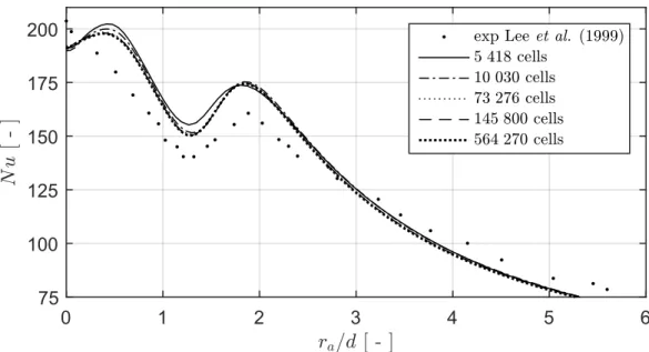
3.8 Mesh independence . . . 27
3.9 Conclusion . . . 29
4 Results and discussion of validation 30 4.1 Comparison of turbulence models . . . 30
4.2 Review of thek-ω SST and Transition SST turbulence models . 33 4.3 Model sensitivities . . . 35
4.4 Numerical correlation with experiments . . . 41
4.5 Conclusion . . . 46
5 Setup of numerical model application 48 5.1 Comparison with previous work . . . 49
5.2 Spike tip model setup . . . 51
5.3 Spike tip pressure drop . . . 55
5.4 Geometric sensitivities . . . 56
5.5 Parametric set . . . 59
5.6 Conclusion . . . 62
6 Results and discussion of model application 63 6.1 Geometric parameters . . . 63
6.2 Fluid property assumption . . . 64
6.3 Receiver thermal eciency . . . 65
6.4 Flux prole parameters . . . 66
6.5 Cycle eciency tool . . . 71
6.6 Conclusion . . . 75 7 Conclusion 76 7.1 Contribution . . . 76 7.2 Recommendations . . . 78 Appendices 80 A HPC automation 81 A.1 Job submission command (HPC interaction) . . . 81
A.2 Fluent TUI commands for validation simulations . . . 82
A.3 Fluent TUI commands for application simulations . . . 84
A.4 User dened ux boundary condition . . . 86
B Flat plate impinging round jet validation 88
C Surface distribution plots 90
List of References 92
List of Figures
1.1 Diagram of a typical CSP central receiver Rankine cycle power plant 2 1.2 Schematic diagram of the SUNSPOT cycle . . . 3 1.3 A drawing of SCRAP with the left side sectioned . . . 4 1.4 A sectioned drawing of the spike showing the air's ow path . . . . 4 1.5 Spike view factor or level of exposure to the surroundings . . . 6 2.1 A cross section of an impinging jet on a at surface . . . 10 2.2 Typical at plate jet impingement N u distribution at dierent
nozzle distances from the surface . . . 12 2.3 Impinging jet Nusselt numbers at Re= 23 000 . . . 14
3.1 A schematic diagram of the concave hemisphere jet impingement experimental setup . . . 19 3.2 Geometric parameters and mesh segmentation of the computational
domain . . . 22 3.3 A coarse mesh of 5176 cells where d= 34 mm and L/d= 4 . . . 23
3.4 Convergence of ymax+ with increasing mesh cell count . . . 27 3.5 Convergence of two values of interest with increasing mesh cell count 28 3.6 Nusselt number distributions for increasing cell count . . . 28 4.1 Nusselt number distributions for the less accurate numerical models
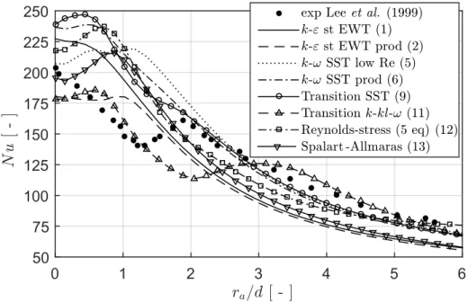
on L4_d3_50 . . . 31 4.2 Nusselt number distributions for the more accurate numerical
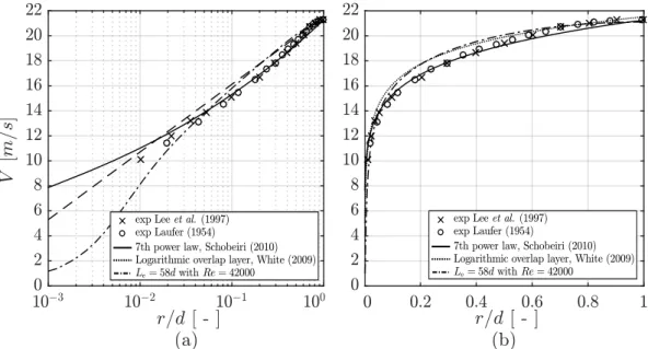
models on L4_d3_50 . . . 32 4.3 Fully developed pipe ow velocity proles along the (a) logarithmic
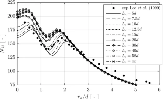
dimensionless radius and (b) linear dimensionless radius . . . 37 4.4 N u distributions resulting from varying pipe ow development
lengthsLe for L4_d3_50 . . . 38
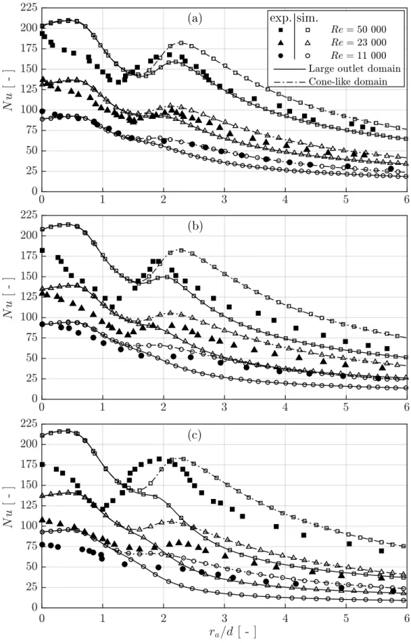
4.5 Contour maps for L4_d1_50 illustrating the outlet region sensitivity 39 4.6 Nusselt number distributions for two dierent diameter ratios . . . 40 4.7 Nusselt number distributions atL/d= 2in both numerical domain
types . . . 42 4.8 Nusselt number distributions atL/d= 4in both numerical domain
types . . . 43 4.9 Nusselt number distributions at L/d = 10 in both numerical
domain types . . . 44 xi
xii LIST OF FIGURES
5.1 Nusselt number distribution comparison for dierent nozzle diameters, d . . . 50 5.2 Comparison of havg by Lubkoll (2017) and current study for
dierent nozzle diameters . . . 50 5.3 Geometry and boundary conditions of the computational domain . 53 5.4 Geometric depiction of SCRAP spike tip with a nozzle . . . 53 5.5 Comparison of ∆ptot by calculation and simulation for dierent
nozzle diameters . . . 56 5.6 Pressure drop over spike tip region using dierent nozzle slope
anglesα for a nozzle diameter of d= 5 mm . . . 57
5.7 Pressure drop and heat transfer coecient over spike tip region using dierent nozzle-to-surface distances,L, for a nozzle diameter of d= 8 mm . . . 58
5.8 A contour map of total gauge pressure . . . 58 5.9 Pressure drop and heat transfer coecient over spike tip region
using dierent nozzle diameters, d, for a distance ratio ofL/d= 2 . 59
5.10 Graph of the four dierent absorbed solar ux q˙00sol proles . . . 61
6.1 Average heat transfer coecient, havg, and pressure drop, ∆p, for
dierent nozzle diameters, d, and nozzle-to-surface distances, L . . 64 6.2 Heat transfer coecient, h, and pressure drop, ∆p, for dierent
nozzle diameters,d, comparing uid property assumptions . . . 65 6.3 A comparison of the application of a uniform ux and a cosine ux
prole with the same area-weighted averages . . . 67 6.4 Thermocline and path lines showing the dierence between the
uniform ux BC and the cosine ux prole BC . . . 68 6.5 Tavg,sandηrecvs. dshowing the signicance of considering radiation
losses . . . 69 6.6 Tavg,s and ηrec vs. d showing the results for dierent energy inputs . 71
6.7 Flow diagram showing the dierent points in the hybrid CSP/gas Brayton cycle . . . 72 6.8 ∆prec,tip and Ts,max vs. d showing the results for dierent energy
inputs . . . 74 6.9 ηth and SF C vs. d showing the results for dierent energy inputs . 74
B.1 Nusselt number distributions on a at plate for model comparison . 88 B.2 Nusselt number distributions on a at plate at dierent Re . . . 89 C.1 N u distributions along the concave surface of the spike tip . . . 90 C.2 Surface temperature,Ts, distributions along external surface of the
end cap . . . 91 Stellenbosch University https://scholar.sun.ac.za
List of Tables
3.1 Naming convention for the 45 experimental cases . . . 21
3.2 Air properties at 286.15 K and 1 bar. . . 25
4.1 Table of percentage dierences between simulation and experimen-tal N uavg . . . 46
5.1 Assumptions and input parameters . . . 52
5.2 Pressure drop calculation contributions . . . 55
5.3 Pressure drop at dierent nozzle diameters . . . 56
5.4 Variations of ux inputs to model . . . 60
Nomenclature
Constants σ = 5.6703×10⁻⁸W/(m2K4) Abbreviations BC Boundary condition BSL Baseline CC Combined cycleCFD Computational uid dynamics CPU Central processing unit
CR Central receiver
CSP Concentrating solar power DNI Direct normal irradiation DNS Direct numerical simulation EWT Enhanced wall treatment HPC High performance computer HTF Heat transfer uid
LCOE Levelised cost of electricity LES Large eddy simulation OCGT Open cycle gas turbine
PC Personal computer
PV Photovoltaic
RANS Reynolds-averaged Navier-Stokes RNG Re-normalised group
RSM Reynolds-stress model SFC Specic fuel consumption
xiv
xv SST Sheer-stress transport
SUNSPOT Stellenbosch University solar power thermodynamic cycle TUI Text user interface
UDF User-dened function Variables
A Area. . . [m2]
arg1 Blending function argument . . . [−]
C N ucorrelation constant . . . [−]
Cf Skin friction coecient . . . [−]
cp Specic heat capacity . . . [kJ/(kg K)]
Cp Pressure coecient . . . [−]
d Nozzle or pipe diameter . . . [m]
D Diameter of the hemispherical impingement surface . . . [m]
d/D Curvature intensity. . . [−]
f Fuel to air ratio . . . [−]
F View factor . . . [−]
F1 Blending function. . . [−]
h Heat transfer coecient . . . [W/(m2K)]
I Turbulent intensity . . . [%]
k Thermal conductivity, Turbulent kinetic energy . . . [W/(m K) , m2/s2]
L Nozzle/pipe-to-surface distance . . . [m]
Le Entrance length . . . [m]
L/d Dimensionless nozzle/pipe-to-surface distance . . . [−]
˙ m Mass ow rate. . . [kg/s] m P r exponent in N ucorrelation . . . [−] n Reexponent in N u correlation. . . [−] N u Nusselt number . . . [−] p Pressure . . . [Pa] P r Prandtl number . . . [−] ˙
Q Heat transfer rate . . . [W] ˙
xvi NOMENCLATURE
q Thermal energy per unit mass ow . . . [kg/(kW h)]
Re Reynolds number (dV /ν) . . . [−]
r Radial distance from stagnation point . . . [m]
ra Radial arc length from stagnation point (curved surfaces) [m]
SF C Specic fuel consumption. . . [kg/(kW h)]
T Temperature. . . [K]
U Fluid velocity . . . [m/s]
V Velocity. . . [m/s] ¯
V Mean nozzle/pipe exit velocity. . . [m/s]
w Work per unit mass ow . . . [kJ/kg]
y+ Dimensionless distance from wall . . . [−]
Z Jet pipe length . . . [m]
α Slope angle of nozzle . . . [ °or rad]
αopt Absorptivity of receiver surface . . . [−]
γ Intermittency or Heat capacity ratio . . . [−]
ε Emissivity or Turbulent dissipation rate . . . [− or m2/s3]
εopt Emissivity of receiver surface . . . [−]
η Eciency. . . [−]
θ End cap surface angle (0at stagnation point) . . . [ °or rad]
µ Dynamic viscosity . . . [kg/(m s)]
ν Kinematic viscosity. . . [m2/s]
νt Eddy-viscosity. . . [m2/s]
ξ Pressure loss coecient . . . [−]
ρ Density . . . [kg/m3]
σ Stefan-Boltzmann constant . . . [W/(m2K4)]
φ An array of constants . . . [−]
ω Specic turbulent dissipation rate . . . [1/s] Ω Vorticity . . . [1/s]
Subscripts
0 Stagnation
a Ambient
xvii
al Allowable
avg Average (area weighted)
b Combustion c Compressor e Entrance exp Experimental f Air g Gas in Inlet j Nozzle/pipe exit loss Loss m Mechanical max Maximum
nat Natural convection
net Net opt Optical out Outlet rad Radiation rec Receiver s Surface sim Simulation sky Sky sp Spike
sol Solar absorbed
t Turbine
tc Turbine to compressor
th Thermal
tip Tip
tot Total
Chapter 1
Introduction
1.1 Background
Renewable energy has, in recent years, seen rapid development towards reducing costs and increasing eciencies of existing technologies. New innovations in other technologies, such as concentrating solar power (CSP), are also experiencing signicant recent growth.
Photovoltaic (PV) energy and wind energy are signicant players in the necessary global sustainable energy transition and CSP, although not as widely adopted, has seen rapid growth since 2006. The lag behind other renewable technologies can be attributed to its relatively high levelised cost of electricity (LCOE). In recent years, CSP has become more economically feasible and has developed into a competitive technology in the renewables industry, which has stimulated growth. The global total CSP capacity was less than 500 MW in
2006 (most of it in the Unites States) and had grown to 4.8 GW worldwide by
the end of 2016 (Sawin et al., 2017).
CSP is a thermal power generation technology in which heat is obtained by concentrating sunlight. To do this, reective surfaces (mirrors) are arranged and/or curved to concentrate solar irradiance onto a receiver. The receiver harnesses high temperature thermal energy which is transported via a heat transfer uid (HTF) to a thermodynamic cycle such as a Rankine cycle. Typically, this thermal energy is captured in synthetic oils or molten salt and exchanged with water/steam to produce electricity through a Rankine cycle such as in a conventional coal-red power station. CSP power plants conventionally make use of parabolic trough collectors. Developments in central receiver (CR) plants (which involve a eld of controlled mirror facets called heliostats that have a point focus at the top of a tower) have further increased eciencies and the economic feasibility of CSP. A simple ow schematic of a state-of-the-art Rankine cycle CR CSP plant with molten salt thermal storage is shown in Figure 1.1.
Managing an electric grid like South Africa's requires supplying the demand without too much curtailment. To achieve this, the grid should have several dierent technologies producing power. Some technologies (such as conventional coal-red power plants) provide a base load, others (such
2 CHAPTER 1. INTRODUCTION
Figure 1.1: Diagram of a typical CSP central receiver Rankine cycle power plant (Augsburger, 2013)
as gas turbines) provide peak load. There are also technologies supplying intermediate load. In an electric grid, the utility operator must manage the suppliers to meet demand without excess curtailment. The grid must have sucient (with a safety factor) production capacity to meet the highest peak demands.
Gas turbines have rapid response times and can therefore be rapidly commissioned by a utility operator during peak demand periods. A gas turbine typically pressurises ambient air via a compressor, after which fuel is added and the air-fuel mixture is combusted and expanded through a turbine that turns an electric generator. The combustion of fuel simply adds thermal energy to the system. This addition of thermal energy can also be achieved by harnessing concentrated solar energy via a CSP receiver as shown on the left of Figure 1.2. A hybrid solarised gas turbine cycle could provide day-time production with low emissions (solar energy replaces fossil fuel consumption to an extent) and be available for peaking production as a conventional gas turbine.
The Stellenbosch University Solar Power Thermodynamic (SUNSPOT) cycle is a combined cycle (CC) CSP plant concept that is being utilised for several research studies at Stellenbosch University and can be congured in several ways. A CC power plant typically has a conventional open cycle gas turbine (OCGT), also known as a Brayton cycle, and a conventional steam turbine cycle, also known as a Rankine cycle. The exhaust gas from the OCGT contains excess usable heat that is recovered in the boiler stage of the Rankine cycle. Thermal energy storage is a signicantly less expensive method of storing energy than electrochemical storage (batteries). The use of thermal energy storage in the SUNSPOT cycle shows the potential for asynchronous production (gas turbine for day-time production and Rankine cycle with stored thermal energy for night-time production).
The conguration of the SUNSPOT cycle shown in Figure 1.2 proposes the use of a pressurised air receiver for the gas turbine (Brayton cycle) with rock bed thermal storage between the Brayton and Rankine cycles (Kröger, 2012).
1.1. BACKGROUND 3
Figure 1.2: Schematic diagram of the SUNSPOT cycle (Kröger, 2012)
A pressurised air receiver could be placed between the compressor and turbine to be used as a pre-heater to oset (or even eliminate) fuel consumption in a hybrid CSP/fuel gas turbine. With the turbo machinery running at full load, the solarised hybrid gas turbine would obtain its thermal input from a combination of the CSP receiver (as a pre-heater) and the combustion of fuel (as a subsidy to obtain the required turbine inlet temperature). The resulting reduction in fuel consumption is desirable for two reasons, namely:
A reduction in the combustion of natural gas results in a reduction of carbon-equivalent emissions, and
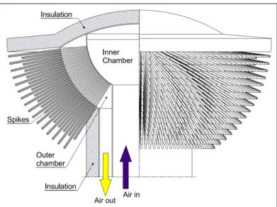
Solar energy is a free source of energy that can oset fuel expenses. The Spiky Central Receiver Air Pre-heater (SCRAP) was proposed by Kröger (2008). Lubkoll (2017) conducted an overall performance analysis of this innovative design. It is categorised as a closed volumetric pressurised air receiver. The receiver is proposed to be situated between the compressor and turbine of the Brayton cycle where the compressed air is heated in the multitude of spikes (see Figure 1.3) that point toward the heliostats. The performance analysis by Lubkoll (2017) included lab-based experimental work on a single spike and a numerical performance analysis. His research showed that the receiver has high potential, but further work is required to bring the concept to a commercialisable state.
Figure 1.4 shows the air ow in a single spike. The spike is made of two concentric pipes with a concave hemispherical dome (further referred to as the end cap or tip) at the end of it. The inner tube is, at its base, connected to the inner chamber at the top of the tower where the unheated compressed air is distributed into all the spikes. The air exits the inner tube at the spike tip as a jet and impinges against the end cap, cooling the end cap and heating the air. The end cap causes the ow to turn around and enter the nned channels where it continues to absorb heat in channel ow. Exiting the nned section into the outer chamber, the heated air then travels either to the combustion chamber for further heating or directly to the turbine.
4 CHAPTER 1. INTRODUCTION
Figure 1.3: A drawing of SCRAP with the left side sectioned (Kröger, 2008)
Figure 1.4: A sectioned drawing of the spike showing the air's ow path (Kröger, 2008)
Lubkoll (2017) recommended that further work should be done on the impinging jet cooling in the spike tip. The current study is based on this recommendation to obtain further insight into the local eects of the cooling mechanism, thereby exploring its eects on the performance of the receiver.
1.2 Problem statement
Lubkoll (2017) shows in his ray-tracing analysis that the end cap experiences a solar ux distribution that is at a maximum at its centre and a minimum where it connects to the rest of the spike. This is predominantly due to cosine losses caused by the curvature of the hemisphere, with the assumption of small heliostats for better penetration into the spiky structure. The area that experiences the highest ux requires the most cooling. Introducing a nozzle at the end of the inner tube of the spike causes the ow to accelerate, increasing the heat transfer capabilities of the jet, particularly in the centre where it impinges in the maximum ux region. The exploitation of the excellent heat transfer characteristics of jet impingement to cool the end cap (which
1.2. PROBLEM STATEMENT 5 experiences the maximum solar ux) forms one of the bases of the concept of the SCRAP.
The SCRAP receiver is conceptualised to be a volumetric receiver whereby the maximum surface temperature occurs deep in the structure and surfaces exposed to the surroundings are at a lower temperature than the HTF outlet temperature. This results in a reduction in radiative and convective losses to the surroundings without compromising the outlet temperature of the receiver, and higher eciencies are thus achievable.
Introducing a nozzle to increase heat transfer at the spike tip will increase the thermal eciency of the receiver. However, it will induce an increased pressure drop over the receiver which would reduce the eciency of the gas turbine cycle. The pressure drop caused by introducing a nozzle is due to the ow acceleration and sudden expansion where no venturi diuser is used to recover the dynamic pressure. The dynamic energy in the jet (high velocity) is what causes the high heat transfer capabilities, so diusing the jet to recover dynamic pressure reduces the heat transfer coecient. This describes the fundamental coupling of pressure drop and heat transfer coecients in thermo-uid mechanics. They are, however, not coupled linearly and they each aect the gas turbine cycle eciency to dierent extents.
Lubkoll (2017) predicted that the thermal eciency,ηth, of the receiver can
exceed 80 %. This thermal eciency does not take pressure drop into account,
so to quantify the performance of the receiver for the application to a Brayton cycle, the pressure drop must be considered.
Thermal losses include convection (natural and forced) and radiation losses. The receiver is highly sensitive to wind, even at low wind speeds, due to the large surface area that is exposed to passing wind (Lubkoll, 2017). The conductive losses to the tower are considered to be negligible. With higher material temperatures, radiation losses increase rapidly. Radiative losses (shown in equation 1.1) are proportional to the dierence between the fourth powers of the material surface and the equivalent sky temperatures.
˙
qrad00 =F εσ(Ts4−Tsky4 ) (1.1)
One way to reduce thermal losses to the surroundings is to reduce the surface temperature of the material that is most exposed to the surroundings. Figure 1.5 shows that the spike tip is the main contributor to radiative losses since its view factor F to ambient is assumed to be 1 (in reality it would be slightly less than 1) and the spike cylinder has a negligible view factor and therefore a negligible contribution to radiative losses.
Reducing the spike tip surface temperature could contribute to the desired volumetric eect, where the receiver surface temperatures are lower than the uid outlet temperatures. This eect is desirable because of the reduction in radiation losses while still achieving high outlet air temperatures, resulting in high receiver thermal eciencies (Avila-Marin, 2011). Due to its exposure to the surroundings, the spike tip is the area to focus on when attempting to reduce radiation losses. The material surface temperatures observed by this
6 CHAPTER 1. INTRODUCTION
receiver can exceed 1000◦Cat the spike tip (Lubkoll, 2017). The performance
analysis by Lubkoll (2017) considers1000◦Cas the upper limit so that steel can
be a feasible material. Improving the jet impingement cooling at the spike tip reduces material surface temperatures and hence reduces the radiative losses and vulnerability to materials melting or deteriorating.
Figure 1.5: Spike view factor or level of exposure to the surroundings (Lubkoll et al., 2015)
A high level computational uid dynamics (CFD) model was developed by Lubkoll (2017) to determine the eects of adding dierent size nozzles to the end of the inner pipe. With a constant mass ow rate, a smaller nozzle means higher jet velocity which impinges on the inner surface of the end cap. Lubkoll (2017) observed that the smaller the nozzle diameter, the better the heat transfer and the lower the end cap material temperature, but a decreased nozzle diameter increases pressure drop.
The CFD model developed by Lubkoll (2017) was validated using at plate experimental results and then extended to the spike tip geometry. The model was used to observe the impinging jet heat transfer characteristics and to understand the eect of the nozzle diameter for his further system modelling. The model validation performed by Lubkoll (2017) was sucient for his initial performance analysis, but he recommended that a comprehensive validation study be done on developing a better understanding of the local eects in the impinging jet ow at the spike tip. The local eects are important because of the complexity of the ow characteristics causing the heat transfer, and due to the fact that the end cap experiences a ux distribution and requires local cooling.
In summary, the SCRAP receiver's spike tip produces radiation losses due to its high surface temperature. This temperature, and hence the losses, can be reduced by decreasing the nozzle diameter at the inner tube exit, but this comes at the cost of pressure drop. There are a number of geometric changes that can improve the heat transfer characteristics of the spike tip, but a more comprehensive validation study is required for the development of a CFD model. A validated model would allow for further improvements to be made to the spike tip through parametric observations or an optimisation study.
1.3. MOTIVATION AND OBJECTIVES 7
1.3 Motivation and objectives
This study is divided into two parts. The rst part presents the development and validation of a CFD model, using published experimental data, with relevance to the application of the spike tip jet impingement. The second part applies the validated model to the SCRAP receiver with the intention of gaining insight into the geometric and uid mechanical eects on the receiver's performance.
1.3.1 Numerical model development
The software being utilised is Fluent v17.2 from ANSYS Inc. and an eort will be made to best understand the capabilities of the commercial software. Impinging jet ow is a complicated ow eld to model numerically. There has been little investigation into the behaviour of an impinging jet on a concave hemispherical surface. In recent publications, McDougall et al. (2018) and Craig et al. (2018) present some numerical results for jet impingement heat transfer on a concave hemisphere.
The objective of developing a numerical model is to observe the capability of Fluent to predict, with an acceptable level of accuracy, the local and average heat transfer characteristics of the highly turbulent jet impingement ow eld, using the Reynolds-averaged Navier-Stokes (RANS) turbulence models.
Accurately predicting the turbulent ow using the RANS models will drastically save computational time in comparison to Large-eddy Simulations (LES) or Direct Numerical Simulations (DNS). A successfully validated RANS model would enable the author to perform an extensive parametric analysis on spike tip jet impingement at relatively low computational expense.
1.3.2 Application of model to SCRAP
Lubkoll (2017) introduces the trade-o between pressure drop and heat transfer in the spike tip jet impingement. The smaller the nozzle diameter, the higher the jet impingement heat transfer capability and the higher the pressure drop. Increased heat transfer is desirable for reduced surface temperature (therefore reduced thermal losses to ambient) and higher receiver eciency, but increased pressure drop is unwanted because it decreases the pressure ratio of the turbine and therefore decreases the gas turbine cycle eciency. This trade-o forms the basis of part two of the current work.
Given that a suciently validated CFD model is developed for concave hemispherical jet impingement, it could be used to study the eects of geometric alterations within the spike tip. A geometric sensitivity study will give insight into the important parameters to consider in a parametric analysis, which would permit the selection of a design that improves the eciency of a selected gas turbine cycle and even permit an optimisation study to be performed in further work.
The objective of this part is to compare the validated CFD results to Lubkoll (2017), to gain a better understanding of the sensitivity of certain
8 CHAPTER 1. INTRODUCTION
nozzle geometric parameters, and to perform a parametric analysis with quantication of the gas turbine cycle eciency. Within the parametric set, the design point with the maximum gas turbine cycle eciency (aected by jet impingement heat transfer and pressure drop) is the preferred design. There are also pressure drop limitations in the turbo-machinery and maximum material temperature limitations that are taken into account here.
The insight gained from the parametric analysis as well as the tools presented (CFD model and gas turbine cycle eciency calculation) will be a step closer to having an in depth understanding of the SCRAP receiver and can be used for further work.
1.4 Methodology
After gaining some insight from the extensive pool of jet impingement literature, a numerical RANS CFD model is developed and validated with relevance to being applied to the SCRAP receiver's spike tip jet impingement. The validation process involves numerically replicating (with the information available) the experimental setup of Lee et al. (1999) and determining the capability of Fluent RANS turbulence models to replicate the published experimental heat transfer proles.
The correlation between the experimental and numerical results determines the validity of the model. It is also important to know the model's sensitivities to numerical inputs such as the mesh renement, the size of the numerical domain and boundary conditions. A sensitivity analysis is therefore presented. The validated numerical model is then used to determine the validity of the high level CFD model used by Lubkoll (2017). Thereafter the reference geometry and environmental parameters presented by Lubkoll (2017) are replicated with the introduction of a nozzle. This nozzle's geometry can have a signicant eect on pressure drop and heat transfer. A sensitivity analysis on some geometric parameters is performed to determine the eect of these parameters. These results lead to a parametric analysis performed to obtain insight into the eect of certain parameters on the eciency of a gas turbine cycle.
A gas turbine cycle eciency calculation is presented as a tool with the inclusion of receiver thermal eciency, pressure drop in the receiver and fuel consumption to get to the required turbine inlet temperature. Assumptions are used with a reference base case to present an example of the benets of quantifying the performance of the receiver in terms of gas turbine cycle eciency.
The purpose of the study is not to select improved design parameters for the spike tip, but rather to present a tool that can be used to simulate the complicated spike tip jet impingement. This tool can be used as part of a design improvement study that considers all parameters of the receiver's design and quanties the receivers performance increase in terms of an improvement to the cycle eciency of the gas turbine it is a part of.
Chapter 2
Review of impinging jet cooling
A literature review on the jet impingement cooling mechanism is conducted with the concave hemispherical impingement surface eects in mind. Other necessary literature is reviewed in subsequent chapters where necessary. This review serves to present the necessary background knowledge of jet impingement ow that is relevant to the practical application in question.
2.1 Introduction to jet impingement
Impinging jet cooling involves a conned stream of uid exiting a nozzle or a pipe as a jet and impinging on a target surface to heat or cool the surface. The uid either removes heat from or transfers heat to the surface, depending on a positive of negative temperature dierence.
A heat transfer coecient is, in general, aected by: local uid and solid properties at the interface, a local temperature dierence between the uid and solid, local ow velocity, and local turbulent intensity. The reason that the jet impingement mechanism displays heat transfer coecients that are superior to most other mechanisms is because of the fact that the uid is forced against the impingement surface at a high velocity with relatively small boundary layer thickness and high levels of turbulence.
Impinging jet cooling is a commonly used cooling mechanism for engineering applications such as turbine blade cooling (Colucci and Viskanta, 1996), manufacturing processes and cooling of electronic equipment (Behnia et al., 1998) where high heat transfer coecients are required.
The ow eld of an impinging jet consists of three major regions, shown in Figure 2.1. In the free jet region, the jet width increases as it gets further from the nozzle and the average jet velocity decreases. This is due to turbulence being introduced by the entrainment of surrounding uid into the jet (a mixing region). The stagnation region is where the uid is forced to change direction from orthogonal to the surface to parallel. The stagnation point is the point on the surface at the centreline of the jet, around which the uid velocity approaches 0 m/s. The stagnation region ends where the parallel component
of the uid velocity reaches its maximum (where the orthogonal component is
0 m/s). A convective wall jet follows in the wall jet region, further transferring
10 CHAPTER 2. REVIEW OF IMPINGING JET COOLING
heat to or from the surface. Jet energy is further dissipated to the surrounding uid as the wall jet progresses.
stagnation point. Dewan et al.[3]reviewed on the current status of computation of turbulent impinging jet. Due to the lack of gener-ality in the reported data they could not assess the accuracy of different LES computations. They found that the hybrid RANS/LES gave good results compared to the simple RANS-based models and the use of an appropriate SGS model gave accurate prediction. This is due to the assumption of isotropy of eddy viscosity-based model
that is not valid in the impinging region. The poor results of RANS-based models may be due to the involvement of a number of arbitrary coefficients. An optimized selection of coefficients may give good result in one region and fail to do so in the other region. In addition to this, poor performance of wall function in the stagna-tion region and the methodology of time averaging are also the reasons for the poor performance of RANS-based models.
In one of the early experimental studies, Vader et al.[4] con-ducted an experimental work for the surface temperature and heat
flux distributions on aflat, upward facing, constant heatflux sur-face cooled by a planar impinging jet. They found that the results were sensitive to the variations in the stagnation line velocity gradient and the Prandtl number. Local convection heat transfer coefficient distributions along a constant heatflux surface experi-encing impingement by two, planar, free-surface jets of water were obtained in an experiment by Slayzak et al.[5]. Two velocity ratios were considered keeping the other parameters constant. They found that with decreasing velocity ratio, impingement heat transfer coefficients beneath the weaker jet were reduced by the effects of crossflow imposed by the stronger jet. Using a thermal imaging technique, Lytle and Webb[6]analyzed experimentally the local heat transfer characteristics of air jet impingement at jet-to-plate spacings of less than one jet diameter. They gave relation-ship of stagnant Nusselt number with Reynolds number and jet-to-plate spacing as NuStRe1=2and Nust ðz=dÞ0:288respectively. In
an experimental study for a two-dimensional air jet impinging onto a vertical impingement plate, Tu and Wood[7]used a wider range of Reynolds number, nozzle-to-impingement plate height to nozzle gap ratio as compared to the previous studies. They found the pressure distributions nearly Gaussian that was independent of Reynolds number. They used a range of Preston tubes and Stanton probes out of which the smallest probe (Stanton probe of size 0.05 mm) gave the best result for the wall shear stress. Cziesla et al.
[8]concluded that the velocity profile at the nozzle exit as a reason for the deviation of the stagnation point Nusselt number from the experimental values. An increase in Nusselt number at the edges of abscissa was observed due to thinning of boundary layer caused by head-on collision between neighboring wall jets. Lin et al.[9], in an experimental study on heat transfer behaviors of a confined slot jet impingement, found that the stagnation, local and average Nusselt numbers were affected by jet Reynolds number while it was insignificantly influenced by the nozzle-to-plate spacing. Yang and Shyu[10]concluded that the positions of maximum local Nusselt number and the maximum pressure move downstream if the confinement plate inclination is increased. The maximum Nusselt number got decreased and the local Nusselt number in the down-stream location got increased with increase in inclination of confinement plate. In addition to this, it was found that the incli-nation has a significant effect on the recirculation region. Maurel and Solliec[11]developed a test bench with variable geometry; they used LDV (laser Doppler velocimetry) and PIV (particle image velocimetry) to analyze the development of the jet for different geometrical configurations. They concluded that the characteristic height of the impinging zone remained close to 12% to 13% of the jet-to-plate spacing, irrespective of the Reynolds number and the jet width. Theflowfield of plane impinging jets at moderate Rey-nolds numbers was computed using LES with dynamic Smagor-insky model by Beaubert and Viazzo[12]. They studied the mean velocity, the turbulence statistics along the jet axis and at different vertical locations. The effect of the jet exit Reynolds number on near and farfield structure is significant between 3000 and 7500. In a numerical study of plane turbulent impinging jet in a confined space using DNS, Hattori and Nagano[13] noticed that for low nozzle-to-plate distances, a second peak appears in the local Nus-selt number and skin friction coefficient distribution along the
Nomenclature
Roman symbols
Gn production by shear (Eq.(5))
h;H dimensional and non-dimensional nozzle-to-plate spacing, respectively
k;kn dimensional and non-dimensional turbulent kinetic energy, respectively
p static pressure
p0 ambient pressure
P non-dimensional pressure Pr Prandtl number,n=a
Ret turbulent Reynolds number,k2=n~ε Rey non-dimensional distance,pffiffiffiky╱n
Re Reynolds number,U0w=n
T;q dimensional and non-dimensional temperature, respectively
ui;Ui dimensional and non-dimensional mean velocity,
respectively
U0 average inlet jet velocity
w jet width
xi;Xi dimensional and non-dimensional Cartesian
coordinates, respectively
Greek symbols
a;at;at;nlaminar, turbulent and non-dimensional turbulent
eddy diffusivity, respectively
~ε;~εn dimensional and non-dimensional modified
turbulent kinetic energy dissipation rate, respectively
n;nt;nt;n laminar, turbulent and non-dimensional turbulent
kinematic viscosity, respectively
u;un dimensional and non-dimensional rate of specific
dissipation
r density offluid
Fig. 1.Schematic diagram of an impinging jet.
A.M. Achari, M.K. Das / International Journal of Thermal Sciences 98 (2015) 332e351 333
Figure 2.1: A cross section of uniform velocity prole jet impinging on a at surface (Achari and Das, 2015)
The highly turbulent ow being forced upon the surface, in conjunction with a temperature dierence between the uid and the surface, results in elevated heat transfer coecients in comparison to other forced convection heat transfer mechanisms.
In the case of the SCRAP receiver, the end cap is subjected to a high solar ux and the purpose of the receiver is that the air ow inside the spikes absorb as much of that heat as possible, while reducing the thermal losses to ambient as much as possible. The design is structured to have a large surface area for heat transfer, hence, the multitude of spikes. Much of the heat transfer occurs in the nned section of the spike, but a substantial air temperature rise is observed due to jet impingement in the spike tip, where heat is transferred from the end cap (the impingement surface) to the compressed air exiting the nozzle at the end of the inner pipe (Lubkoll, 2017).
This review is conducted to better understand the impinging jet cooling mechanism in the context of the SCRAP receiver and how dierent design parameters or ow conditions aect heat transfer. These design parameters and ow conditions include: Reynolds number, nozzle-to-surface distance, and concave impingement surface. Some geometric sensitivities, the second peak phenomenon, and numerical turbulence modelling of jet impingement are reviewed.
2.2 Reynolds numbers and typical Nusselt
numbers
Reynolds numbers mentioned henceforth are based on the nozzle diameter, d, and mean nozzle exit velocity, V¯, as Re =ρdV /µ¯ where ρ is the density and
µ is the dynamic viscosity of the uid at the nozzle exit. Smooth pipe ow is considered turbulent at Re ≥ 2300 (Faisst and Eckhardt, 2004; Kerswell,
2.3. SECOND PEAK PHENOMENON 11 2005) and free jets are considered turbulent ow for Re ≥ 100 (Schabel and
Martin, 2010).
To characterise the heat transfer between a solid and a uid, the Nusselt number, N u, shown in equation 2.1 is typically used. It is the heat transfer coecient, h, between the solid and uid, non-dimensionalised by a characteristic length, d, and the thermal conductivity of the uid,k. TheN u is therefore a measure of the ratio of convective heat transfer, h [W/(m2K)],
and the conductive heat transfer, k/d [W/(m2K)]. The characteristic length,
d, in the case of this jet impingement study is the nozzle diameter or jet pipe exit diameter.
N u=hd/k (2.1)
The heat transfer coecient is calculated as shown in equation 2.2 where
˙
q00 is the local surface heat ux on the impingement surface. Notice that the temperature dierence in question is between the impingement surface local temperature and the average uid uid temperature at the nozzle exit.
h= ˙q00/(Ts−Tj) (2.2)
Average surface Nusselt numbers can range from 2 to 1700. Jets from
laminar pipe ow with nozzles close to the surface can produce Nusselt numbers from 2 to 20 (Zuckerman and Lior, 2006) while Rahimi et al. (2003) observed local Nusselt numbers up to 1700 from a supersonic jet. These are extreme
cases of low and high Nusselt numbers, but typically Reynolds numbers of
4000 to 80 000 are used in jet impingement cooling applications with Nusselt
numbers ranging from 50 to 200 (Zuckerman and Lior, 2006).
There are several empirical relationships for jet impingement Nusselt numbers and they typically include the Prundtl number,P r, Reynolds number, Re, and an empirical function, f(L/d), of the ratio of the nozzle-to-surface
distance, L, and the nozzle diameter, d. The form of such an empirical relationship is described by Zuckerman and Lior (2006) and shown in equation 2.3 where C, n and m are constants.
N u=C RenP rmf(L/d) (2.3)
For at plate jet impingement, increasing average Nusselt numbers are typically observed when the nozzle-to-surface distance, L, is decreased or when the Reynolds number, Re, is increased. An increased Reynolds number is attributed to an increased mass ow rate, m˙, and/or a decreased nozzle
diameter, d, (see equation 2.7).
2.3 Second peak phenomenon
A surface Nusselt number plot along the radial direction of a round jet impinging on a at surface typically has a global maximum at the stagnation point and decreases rapidly along the radial direction. Figure 2.2 shows the typical expected N uradial distribution from the stagnation point of at plate
12 CHAPTER 2. REVIEW OF IMPINGING JET COOLING
jet impingement heat transfer. It is common to observe a second peak on such a distribution in certain ow condition ranges. This is observed in Figure 2.2 with a nozzle distance ratio, L/d, of 2.
r/d [-] 0 1 2 3 4 5 6 N u [-] 40 60 80 100 120 140 160 L/d= 2 L/d= 6 L/d= 10 L/d= 14
Figure 2.2: Typical at plate jet impingementN udistribution from the stagnation
point at dierent nozzle distances from the surface, L, with Re = 23 000
(experimental results by Baughn and Shimizu (1989))
There have been several propositions made by researchers as to the reason for this phenomenon known as the secondary peak. Some early observations before the 21st century led to a number of conclusions. Gardon and Akrat (1965) state that the secondary peak is due to the thinning of the boundary layer due to the speeding up of the ow as it changes direction, which is accentuated as the nozzle-to-surface distance is decreased. Lytle and Webb (1994), similarly, concludes that the phenomenon is due to a peak in turbulence in the boundary layer because of accelerated ow, but also attributes it to the entrainment of ambient or free-stream uid into the jet. This changes the uid temperature and increases heat transfer when the entrainment region impinges the surface. Fox et al. (1993) claim that the large eddies generated by the interaction between the jet and the surrounding air introduce vortices to the wall jet, changing the local temperatures and thus causing a secondary peak. Kataoka et al. (1987) also determined that the increase in heat transfer is due to the large vortices that aect the ow structure.
With further developments in CFD turbulence models and Large Eddy Simulations (LES) the complexity of jet impingement ow can be observed in more detail for a better understanding. Hadziabdic and Hanjalic (2008) performed LES on jet impingement to better understand the two peaks. They conclude that there is a recirculation of uid in the region between the two peaks, which is heated, reducing its cooling capability and thus reducing the local Nusselt number. The local minima accentuates the second peak, which is not only due to the recirculation, but also the elevated advection caused
2.4. NOZZLE-TO-SURFACE DISTANCE AND NOZZLE DIAMETER 13 by accelerated ow in the wall jet. Uddin et al. (2013) also performed LES simulations with a particular interest in understanding the secondary peak phenomenon. It was found that there is a region on the impingement surface that experiences hot and cold spots caused by the surrounding large eddies. This, in conjunction with the accelerated ow that changes the development of the thermal boundary layer, is concluded by Uddin et al. (2013) to be the cause of the secondary peak. They further observe that the local second maxima typically occur at1.4≤r/d≤2.8, wherer is the local radial distance from the stagnation point.
2.4 Nozzle-to-surface distance and nozzle
diam-eter
The nozzle-to-surface distance, L, does not aect Reynolds number, but the nozzle diameter, d, does. It is seen in equation 2.7 that the Reynolds number is directly proportional to mass ow rate and inversely proportional to the nozzle diameter, d. ˙ m=ρAV¯ (2.4) A= πd 2 4 (2.5) ν= µ ρ (2.6) Re= ¯ V d ν = ρ ¯ V dA µA = md˙ µπd42 = m˙ µπd4 (2.7)
The results shown in Figure 2.3 from a study conducted by Lee et al. (2004) show the eect of changing nozzle diameters for at plate impinging jet ow. They conclude that an increasing nozzle diameter produces higher heat transfer at and around the stagnation point, with negligible dierences observed down-stream at radius-to-diameter ratios r/d >0.5. It is noted that
for practical applications, this does not mean that a larger nozzle is better, because increasing the nozzle diameter means the mass ow rate must increase to achieve a constant Reynolds number.
Lee et al. (1997, 2004) and Kataoka et al. (1987) found that the maximum stagnation point Nusselt number is achieved at a nozzle-to-surface distance of L/d≈7 on a at plate.
14 CHAPTER 2. REVIEW OF IMPINGING JET COOLING
Figure 2.3: Impinging jet Nusselt numbers at Re = 23 000 (a) Stagnation point
Nusselt numbers for dierent nozzle diameters and nozzle-to-surface distances (b) Radial Nusselt number distribution for dierent nozzle diameters at L/d = 6 (Lee
et al., 2004; Yan, 1993)
2.5 Concave surface eects
Most of the available literature on jet impingement heat transfer refers to at plate impingement. The geometry of the SCRAP receiver end cap is a hemisphere and the curvature of the surface aects the ow structure and heat transfer. It is assumed that the surface curvature acts against the uid's inertia and helps prevent separation.
Sharif and Mothe (2010) states that surface curvature is able to increase average heat transfer rates by up to 20 % in comparison to at plates. The
curvature intensity, d/D (the ratio of nozzle diameter, d, and curved surface diameter,D), has a signicant eect on the average heat transfer rate. Öztekin et al. (2013) studied this eect with a slot jet impinging on a concave trough. Dierent curvature intensities were tested and it was found that there is an optimal curvature intensity that results in a maximum N uavg. The average
Nusselt numbers produced by the at plate (curvature intensity of d/D = 0)
were signicantly less than the curved plates. The curvature eect (forced change of ow inertia due to the curvature) is also said to be accentuated with increasing Reynolds numbers (Yang et al., 1999).
The increased heat transfer capabilities are attributed to the eect that the curvature has on the development of the turbulent boundary layer. The boundary layer is destabilised by Taylor-Görtler vortices, caused by centrifugal forces, which increases turbulent intensity and, hence, heat transfer characteristics (Thomann, 1968).
Gau and Chung (1991) developed two empirical formulae for the average Nusselt number of a 2D slot jet on a concave semi-circular trough surface shown in equations 2.8 and 2.9. The formulae are similar to the form of equation 2.3 with the addition of the curvature intensity.
N uavg = 0.251Re0.68(D/d)−0.38(L/d)0.15 for 6000≤Re≤35 000 8≤D/d≤45.7 2≤L/d≤8 (2.8) Stellenbosch University https://scholar.sun.ac.za
2.6. NUMERICAL TURBULENCE MODELS 15 N uavg = 0.394Re0.68(D/d)−0.38(L/d)−0.32 for 6000≤Re≤35 000 8≤D/d≤45.7 8≤L/d≤16 (2.9) An experimental study on concave hemispherical jet impingement heat transfer was conducted by Lee et al. (1999). This is, to the author's knowledge, the only study done on an axisymmetric concave geometry (other research involving concave surfaces are typically on 2-d slot jets on troughs).
In order to understand the parametric sensitivity, Lee et al. (1999) studied 45 dierent cases. Some of the geometries and ow conditions are similar to that of the SCRAP receiver tip. It is because of these similarities that these experimental results have been selected as the validation case for developing a numerical model. Their experimental setup and results are further introduced in section 3.1.
2.6 Numerical turbulence models
The ow eld of an impinging jet is known to have complex structures with a high level of turbulence and large scale eddies. The vast range of complexities from stagnant ow to large eddies to wall boundary layers brings uncertainties and diculties when utilising RANS turbulence models, but there are several cases in literature where RANS models produce adequate predictions of ow and heat transfer characterisation.
The RANS models of interest for jet impingement include the standard k−ε, re-normalised group (RNG)k-ε, realisablek-ε, standardk-ω, sheer-stress transport (SST) k-ω, Reynolds-stress (RSM) and v2f models. The intricacies
of the numerical models are not studied in detail in the scope of this report, but previous researchers have reviewed the advantages and disadvantages of these models in the context of jet impingement ow.
Using a variation of the standardk-εmodel, Cooper et al. (1993) found that the turbulent kinetic energy, k, around the stagnation point, is over-predicted by an order of magnitude. This results in too much entrainment of the free-stream uid, reducing the jet's momentum and causing the ow acceleration into the wall jet to be reduced. As a result, the wall jet boundary layer is thicker and hence less heat transfer occurs in the wall jet region.
RNG k-ε has additional terms in its transport equations for k and ε that the standard k-ε does not have (Yakhot and Orszag, 1987). Behnia et al. (1998) compared the standard and RNG k-ε models with the v2f model.
The v2f is similar to the standard k-ε, but it does not require any wall
functions as it is valid in the boundary layer (Behnia et al., 1998). It was found that the RNG and standard k-ε models produce similar results, with the re-normalised coecients not improving the over-predicted turbulence. A signicant improvement in ow and heat transfer prediction with thev2f model
in comparison to the k-ε model is found, with v2f results in good agreement
with experimental results. The v2f model is unfortunately not used in this
16 CHAPTER 2. REVIEW OF IMPINGING JET COOLING
academic license server. Special permission is required for the activation of the model.
A study on several variations of the k-ε and k-ω models (excluding SST hybrids) was done by Jarmillo et al. (2012). They conclude that the k-ω, in general, is better at predicting jet impingement ow than the k-ε. They also performed Direct Normal Simulations (DNSs) which, understandably, produced better results that the RANS turbulence models. It was, however, found that the variation of the k-ω model that Yap (1987) proposed, has good agreement with the DNS and experimental results.
RANS turbulence models are pursued and developed because of the computational time that is saved in comparison to LES or DNS. Later, in 2005, Angioletti et al. (2005) compares three of the better impinging jet models, namely, RNGk-ε, SSTk-ωand RSM, using version6.0of the Fluent
commercial software. This study was done on Re in the transition regime from 1000 to 4000 and found that SST k-ω is better for the lower end of the range of Re while RNG k-ε and RSM are better for the higher Re.
Zuckerman and Lior (2006) reviewed the accuracy and computational costs of the k-ε, k-ω, algebraic stress, RSM, SST, v2f, DNS and LES models of
predicting at plate impinging jet heat transfer. LES and DNS models are the most accurate, but the transient nature of the solution method makes the computational time one to two orders of magnitude more than that of the RANS models. The best compromise between accuracy and speed is concluded by Zuckerman and Lior (2006) to be the SST or v2f models.
Rama Kumar and Prasad (2008) used the SST k-ω model in FLUENT v6.2.16 for jet impingement of a row of jets on a concave semi-cylinder. This ow eld entails interference between the jets in the axial direction of the semi-cylinder, but is expected to exhibit similar characteristics to the axisymmetric ow seen in the SCRAP spike-tip. Of the jet impingement CFD work published up to the date of this report, the work by Rama Kumar and Prasad (2008) has, to the author's knowledge, the closest resemblance to the geometry and ow characteristics of the SCRAP's jet impingement ow. They nd that the results produced by the SST k-ω model are in good agreement with the empirical correlations.
Furthermore, Caggese et al. (2013) follow the recommendation of Zuckerman and Lior (2006) and use the SST k-ω model. Their results show good experimental agreement1, with the exception of poor agreement
when L/d = 0.5, which is out of the parametric scope of the validation and
application of the present study.
There are several published works on LES and DNS transient simulation of jet impingement that often, as expected, outperform the RANS turbulence models. One such example is the LES simulations conducted by Uddin et al. (2013) who, as mentioned in section 2.3, study the phenomenon of the secondary N u peak. While these transient simulations produce excellent 1Agreement is within 10 % for area-weighted averageN u (N uavg) and 7 % to 8 % for
stagnation pointN u (N u0)
2.7. CONCLUSION 17 results, they require immense computational time relative to RANS turbulence modelling. The purpose of this study is to determine the adequacy of the RANS models in predicting concave hemispherical jet impingement with relatively little computational time. The transient models are therefore not further reviewed.
Commercial software developers such as ANSYS Inc. who develop
FLUENT have customer support that oers technical assistance with their software packages. They are often challenged by problems that customers present that the software isn't capable of solving. In such a case, the company will often use it as an opportunity to improve the numerical models or make other appropriate improvements. These commercial packages are therefore constantly improving and releasing new versions. In 2016, ANSYS reported on the results of the newly-implemented mechanism in the SSTk-ωmodel. The model produced good correlation with experimental data, including excellent secondary N u peak prediction (ANSYS, 2016).
2.7 Conclusion
The study of impinging jet ow is a signicantly large eld of study with a vast collection of literature. The heat transfer mechanism's ow eld entails a number of complex characteristics that are evidently dicult to model numerically.
In summary, a higher Reynolds number yields better heat transfer (whether a higher mass ow rate is selected or a smaller nozzle). The optimal dimensionless nozzle-to-surface distance is L/d≈7 for a at plate (Lee et al.,
1997, 2004; Kataoka et al., 1987) and is found by Lee et al. (1999) to be
6≤L/d≤8on a concave hemisphere. If the concave hemisphere diameter D is constant, as is the case in this study, the optimal curvature intensity d/D is only achievable by varying the nozzle diameter d.
It is observed that the SSTk-ω model seems to be the preferred numerical model for jet impingement ow predictions, but no literature seems to exist that demonstrates this model's suitability for jet impingement on a concave hemispherical surface.
This review of some of the literature, in the context of the SCRAP's spike tip jet impingement cooling presents a background knowledge of some of the ow complexities, parametric sensitivities and numerical models that will be utilised and further referred to in this analysis.
Chapter 3
Setup of numerical model validation
1
CFD RANS modelling is typically used to model turbulent ow with Reynolds decomposition, rst proposed by Reynolds (1895), which separates the time-averaged and time-uctuating components of the uid ow. The resulting equations, based on the Navier-Stokes equations, form the numerical RANS turbulence models that are used to approximate time-averaged solutions to turbulent uid ow. The numerical predictions of ow elds and heat transfer with CFD is done by discretising the ow domain, applying boundary conditions to that domain and solving a set of equations within the specied discretised numerical environment.
The usability of a CFD model increased by validating it against analytical solutions, experimental data or empirical correlations. This chapter presents the setup of a RANS numerical environment (further referred to as the model) in which a suitable experimental case study by Lee et al. (1999) will be numerically replicated. In the following chapter, the numerical prediction results will be compared to the published experimental results to determine the model's sensitivities and its accuracy2.
Some of the experimental parameters are outside of the scope of the characteristics of SCRAP, nonetheless all of the parameters are analysed to determine the limitations of the model over a wider range of ow characteristics.
3.1 Experimental validation case study
The end cap of the SCRAP receiver is exposed to a non-uniform solar ux distribution. The ux distribution in combination with the expectation of a secondary peak in heat transfer and other localised heat transfer eects of impinging jets can lead to substantial temperature dierentials over the end
1Parts of this chapter have been published in McDougall et al. (2018)
2A number of uncertainties with regard to the experimental environment will be reported
in this chapter. The author has attempted to establish contact with Lee et al. (1999), but was not successful. The uncertainties are reported for completeness sake, but are not deemed to impact on the results reported herein.
18
3.1. EXPERIMENTAL VALIDATION CASE STUDY 19 cap surface. Local eects are vital in determining localised radiation losses and material limitations. It is therefore imperative to validate the local eects.
The experimental setup developed by Lubkoll et al. (2016) was designed to be modular for further alternative experimentation on a single spike and it is available for use by the author. The dome (end cap) at the tip of the spike can be placed in the steam chamber in order to determine average heat transfer coecients and pressure drops of the impinging jet ow with varying pipe diameters. However, an average heat transfer coecient is considered insucient for the current validation process because it does not capture the necessary localised eects. For this reason, it was decided that for the scope of this study, no experiments would be conducted and the results from Lee et al. (1999) are to be used as a case study to develop and validate a CFD model that can be applied to spike tip jet impingement predictions. The details of the experimental case study (Lee et al., 1999) are henceforth introduced.
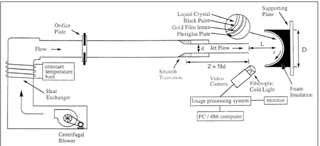
While plenty of experimental and numerical publications have been made on jet impingement, they are typically conned to applying a jet to a standard at plate or curved trough impingement surface. Lee et al. (1999) conducted experiments on an impinging jet on a concave hemispherical surface to determine the eect of several parameters on heat transfer. Their methodology is sound and their non-dimensional geometric and ow parameters are similar to that of the SCRAP spike tip characteristics. This experimental case study is therefore chosen as the validation case study for the present work.
As seen in Figure 3.1, the impingement surface had a thermochromic liquid crystal layer that changed colour locally according to its temperature. A layer of resistive metal was used to induce a uniform heat ux to the concave hemisphere, with the back side insulated. A camera captured images that were analysed by a computer to produce isotherm maps of the surface. These were used to calculate local Nusselt number distributions from the stagnation point. This remote temperature measurement technique was described by Lee et al. (1994) and Lee et al. (1995). They estimated that the Nusselt numbers presented have a maximum uncertainty of 4.5 %.
Figure 3.1: A schematic diagram of the concave surface jet impingement experimental setup (Lee et al., 1999)