Chapter 6: The Fermi Liquid

Chapter 6: The Fermi Liquid

L.D. Landau January 13, 2008

Contents

1 introduction: The Electronic Fermi Liquid 3 2 The Non-Interacting Fermi Gas 5

2.1 Infinite-Square-Well Potential . . . 5

2.2 The Fermi Gas . . . 10

2.2.1 T = 0, The Pauli Principle . . . 10

2.2.2 T ₆= 0, Fermi Statistics . . . 13

3 The Weakly Correlated Electronic Liquid 23 3.1 Thomas-Fermi Screening . . . 23

3.2 Fermi liquids . . . 28

3.3 Quasi-particles . . . 29

3.3.1 Particles and Holes . . . 29

3.3.2 Quasiparticles and Quasiholes at T = 0 . . . 33

3.4 Energy of Quasiparticles. . . 39

4 Interactions between Particles: Landau Fermi Liquid 42 4.1 The free energy, and interparticle interactions . . . 42

4.2.1 Equilibrium Distribution of Quasiparticles at FiniteT . . . 48 4.2.2 Local Equilibrium Distribution . . . 50 4.3 Effective Mass m∗ _{of Quasiparticles . . . . 52}

1 introduction: The Electronic Fermi Liquid

As we have seen, the electronic and lattice degrees of freedom decouple, to a good approximation, in solids. This is due to the different time scales involved in these systems.

τion ∼ 1/ωD ≫ τelectron ∼

¯

h EF

(1)

where EF is the electronic Fermi energy. The electrons may be

thought of as instantly reacting to the (slow) motion of the lat-tice, while remaining essentially in the electronic ground state. Thus, to a good approximation the electronic and lattice degrees of freedom separate, and the small electron-lattice (phonon) in-teraction (responsible for resistivity, superconductivity etc) may be treated as a perturbation (with ωD/EF as an expansion

pa-rameter); that is if we are capable of solving the problem of the remaining purely electronic system.

At first glance the remaining electronic problem would also appear to be hopeless since the (non-perturbative) electron-electron interactions are as large as the combined electron-electronic kinetic energy and the potential energy due to interactions with

the static ions (the latter energy, or rather the corresponding part of the Hamiltonian, composes the solvable portion of the problem). However, the Pauli principle keeps low-lying orbitals from being multiply occupied, so is often justified to ignore the electron-electron interactions, or treat them as a renormaliza-tion of the non-interacting problem (effective mass) etc. This will be the initial assumption of this chapter, in which we will cover

• the non-interacting Fermi liquid, and

• the renormalized Landau Fermi liquid (Pines Nozieres). These relatively simple theories resolve some of the most im-portant puzzles involving metals at the turn of the century. Per-haps the most intriguing of these is the metallic specific heat. Except in certain “heavy fermion” metals, the electronic contri-bution to the specific heat is always orders of magnitude smaller than the phonon contribution. However, from the classical theo-rem of equipartition, if each lattice site contributes just one elec-tron to the conduction band, one would expect the contributions

from these sources to be similar (Celectron ≈ Cphonon ≈ 3N rkB).

This puzzle is resolved, at the simplest level: that of the non-interacting Fermi gas.

2 The Non-Interacting Fermi Gas

2.1 Infinite-Square-Well Potential

We will proceed to treat the electronic degrees of freedom, ig-noring the electron interaction, and even the electron-lattice interaction. In general, the electronic degrees of freedom are split into electrons which are bound to their atomic cores with wavefunctions which are essentially atomic, unaffected by the lattice, and those valence (or near valence) electrons which react and adapt to their environment. For the most part, we are only interested in the valence electrons. Their environment de-scribed by the potential due to the ions and the core electrons– the core potential. Thus, ignoring the electron-electron interac-tions, the electronic Hamiltonian is

H = P

2

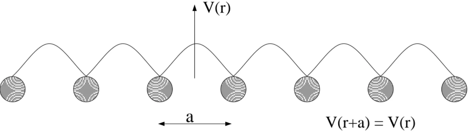
As shown in Fig. 1, the core potential V (r), like the lattice, is periodic

a

V(r)

V(r+a) = V(r)

Figure 1: Schematic core potential (solid line) for a one-dimensional lattice with lattice constanta.

For the moment, ignore the core potential, then the electronic wave functions are plane waves ψ _∼ eik·r. Now consider the core potential as a perturbation. The electrons will be strongly effected by the periodicity of the potential when λ = 2π/k _∼ a

1_{. However, when k is small so that λ}

≫ a (or when k is large, so λ _≪ a) the structure of the potential may be neglected, or we can assume V(r) = V0 anywhere within the material. The

1

Interestingly, when λ∼a, the Bragg condition 2dsinθ≈a≈λ may easily be satisfied, so the electrons, which may be though of as DeBroglie waves, scatter off of the lattice. Consequently states for whichλ= 2π/k∼aare often forbidden. This is the source of gaps in the band structure, to be discussed in the next chapter.

potential still acts to confine the electrons (and so maintain charge neutrality), so V(r) = _∞anywhere outside the material.

Figure 2: Infinite square-well potential. V(r) = V0 within the well, and V(r) = ∞

outside to confine the electrons and maintain charge neutrality.

Thus we will approximate the potential of a cubic solid with linear dimension L as an infinite square-well potential.

V(r) =            V0 0 < ri < L ∞ otherwise (3)

The electronic wavefunctions in this potential satisfy

− h¯

2

2m∇

2_{ψ(r) = (E′}

The normalize plane wave solution to this model is ψ(r) = Y3 i=1   2 L   1/2 sinkixi where i = x, y, or z (5)

and kiL = niπ in order to satisfy the boundary condition that

ψ = 0 on the surface of the cube. Furthermore, solutions with

ni < 0 are not independent of solutions with ni > 0 and may

be excluded. Solutions with ni = 0 cannot be normalized and

are excluded (they correspond to no electron in the state). The

π/L

k_x k_y

k_z

(π/L)3

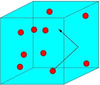
Figure 3: Allowed k-states for an electron confined by a infinite-square potential. Each state has a volume of (π/L)3 in k-space.

eigenenergies of the wavefunctions are

−h¯ 2 ∇2 2m ψ = ¯ h2 2m X i k 2 i = ¯ h2π2 2mL2 n2_x + n2_y +n2_z (6)

and as a result of these restrictions, states in k-space are con-fined to the first quadrant (c.f. Fig. 3). Each state has a volume (π/L)3 of k-space. Thus as L _{→ ∞}, the number of states with energies E(k) < E < E(k) +dE is dZ′ = (4πk 2_dk)/8 (π/L)3 . (7) Then, since E = ¯h_2m2k2, so k2dk = _¯hm2 r 2mE/h¯2dE dZ = dZ′/L3 = 1 4π2   2m ¯ h2   3/2 E1/2dE . (8)

or, the density of state per unit volume is

D(E) = dZ dE = 1 4π2   2m ¯ h2   3/2 E1/2. (9)

Up until now, we have ignored the properties of electrons. How-ever, for the DOS, it is useful to recall that the electrons are spin-1/2 thus 2S + 1 = 2 electrons can fill each orbital or k-state, one of spin up the other spin down. If we account for this spin degeneracy in D, then

D(E) = 1 2π2   2m ¯ h2   3/2 E1/2. (10)

2.2 The Fermi Gas

2.2.1 T = 0, The Pauli Principle

Electrons, as are all half-integer spin particles, are Fermions. Thus, by the Pauli Principle, no two of them may occupy the same state. For example, if we calculate the density of electrons per unit volume

n = Z₀∞D(E)f(E, T)dE , (11)

where f(E, T) is the probability that a state of energy E is oc-cupied, the factor f(E, T) must enforce this restriction. How-ever, f is just the statistical factor; c.f. for classical particles

f(E, T) = e−E/kBT _{for classical particles, (12)}

which for T = 0 would require all the electrons to go into the ground state f(0,0) = 1. Clearly, this violates the Pauli principle.

At T = 0 we need to put just one particle in each state, start-ing from the lowest energy state, until we are out of particles. Since E _∝ k2 in our simple square-well model, will fill up all

k-states until we reach some Fermi radius kF, corresponding to

some Fermi Energy EF

k_x k_y k_z

k

k

Figure 4: Due to the Pauli principle, all k-states up to kF, and all states with energies

up to Ef are filled at zero temperature.

EF = ¯ h2k_F2 2m , (13) thus, f(E, T = 0) = θ(EF − E) (14) and n = Z₀∞D(E)f(E, T)dE = Z₀EF D(E)DE =   2m ¯ h2   3/2 ₁ 2π2 Z E_F 0 E 1/2_DE =   2m ¯ h2   3/2 ₁ 2π2 2 3E 3/2 F , (15)

or EF = ¯ h2 2m 3π2n2/3 = kBTF (16)

which also defines the Fermi temperature TF. Thus for metals,

in which n _≈ 1023/cm3, EF ≈ 10−11erg ≈ 10eV ≈ kB105K.

Notice that due to the Pauli principle, the average energy of the electrons will be finite, even at T = 0!

E = Z₀EF D(E)EdE = 3

5nEF . (17) However, it is the electrons near EF in energy which may be

excited and are therefore important. These have a DeBroglie wavelength of roughly λe = 12.3 A◦ (E(eV))1/2 ≈ 4 ◦ A (18)

thus our original approximation of a square well potential, ig-noring the lattice structure, is questionable for electrons near the Fermi surface, and should be regarded as yielding only qual-itative results.

2.2.2 T ₆= 0, Fermi Statistics

At finite temperatures some of the states will be thermally ex-cited. The energy available for these excitations is roughly

kBT, and the only possible excitations are from filled to

un-filled electronic states. Therefore, only the states within kBT

(EF − kBT < E < EF + kBT) of the Fermi surface may be

excited. f(E, T) must be modified accordingly.

What we need is then f(E, T) at finite T which also satisfies the Pauli principle. Lets return to our model of a periodic solid which is constructed by bringing individual atoms together from an infinite separation. First, just consider a solid constructed from only two atoms, each with a single orbital (Fig. 5). For

1

2

δ

n = -1

δ

n = +1

this system, in equilibrium, 0 = δF = X i ∂F ∂ni δni (19)

electrons are conserved so P

iδni = 0. Thus, for our two orbital

system ∂F ∂n1 δn1 + ∂F ∂n2 δn2 = 0 and δn1 +δn2 = 0 (20) or ∂F ∂n1 = ∂F ∂n2 (21) A similar relation holds for an arbitrary number of particles. Apparently this quantity, the increased free energy needed to add a particle to the system, is a constant

∂F ∂ni

= µ (22)

for all i. µ is called the chemical potential.

Now consider an ensemble of orbitals. We will treat the ther-modynamics of this system within the canonical ensemble (i.e. the system is in contact with a thermal bath, and the particle number is conserved) for which _F = _{E −}T_S is the appropriate potential. The system energy _E and Entropy _S may be written

as functions of the orbital energies Ei and occupancies ni and

the degeneracy gi of the state of energy Ei. For example,

g = 2

E

E

E

g = 4

g = 2

E

g = 4

n = 2

n = 4

n = 1

n = 2

Figure 6: states from an ensemble of orbitals.

E = X

i niEi. (23)

The entropy _S requires a bit more thought. If P is the number of ways of distributing the electrons among the states, then

S = kB lnP . (24)

Consider a set of gi states with energy Ei. The number of

ways of distributing the first electron in these states is gi. For

a second electron we then have gi − 1 ways... etc. So for ni

electrons there are

gi!

ni!(gi − ni)!

possible ways of accommodating the ni (indistinguishable)

elec-trons in gi states.

The number of ways of making the whole system (ie, filling energy levels with Ei 6= Ej) is then

P = Y

i

gi!

ni!(gi − ni)!

, (26)

and so, the entropy

S = kB X i lngi! −lnni! − ln(gi − ni)!. (27) For large n, lnn! _≈ nlnn ₋ n, so S = kB X i gilngi −nilnni − (gi −ni) ln(gi − ni) (28) and F = X i niEi −kBT X i gilngi − nilnni − (gi − ni) ln(gi − ni) (29) We will want to use the chemical potential µ in our thermo-dynamic calculations

µ = ∂F

∂nk

= Ek +kBT (lnnk + 1 − ln(gk − nk)− 1) , (30)

where β = 1/kBT. Solving for nk

nk =

gk

Thus the probability that a quantum state with energy E is occupied, is (the Fermi function)

f(E, T) = 1

1 + eβ(E_k−µ) . (32)

At T = 0, β = _∞, and f(E,0) = θ(µ₋E). Thus µ(T = 0) =

EF. However in general µ is temperature dependent, since it

must be adjusted to keep the particle number fixed. In addition,

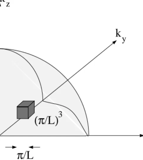
0.0 0.5 1.0 1.5 2.0 ω 0.0 0.5 1.0 1.5 1/(e β ( ω−µ ) +1)

Figure 7: Plot of the Fermi function 1/e−β(ω−µ)_{+ 1 when β = 1/k}

BT = 20 and

µ= 1. Not that at energiesω _≈µthe Fermi function displays a smooth step of width

≈kBT = 0.05. This allows thermal excitations of particles near the Fermi surface.

when T ₆= 0, f becomes less sharp at energies E _≈ µ. This reflects the fact that particles with energies E ₋µ _≈ kBT may

Specific Heat The form of f(E, T) also clarifies why the elec-tronic specific heat of metals is so small compared to the clas-sical result Cclassical = 3₂nkBT. The reason is simple: only the

electrons with energies within about kBT of the Fermi surface

may be excited (about kBT

E_F of the electron density) each with

excitation energy of about kBT. Therefore,

Uexcitation ≈ kBT n kBT EF = nkBT T TF (33) so C _≈ nkB T TF (34)

Then as T _≪ TF (TF is typically about 105K in most metals2)

C _≈ nkB_TT_F ≪ Cclassical ≈ nkB. Thus at temperatures where

the phonons contribute essentially a classical result to the spe-cific heat, the electronic contribution is vanishingly small. In general this holds except at very low T where the phonon con-tribution Cphonon ∼ T3 goes to zero faster than the electronic

contribution to the specific heat.

2

Heavy Fermion systems are the exception to this rule. There TF can be as small as a fraction

Specific Heat Calculation Of course, since we know the free energy of the non-interacting Fermi gas, we can calculate the form of the specific heat. Here we will follow Ibach and L¨uth and Kittel; however, since the chemical potential does depend upon the temperature, I would like to make the approximations we make a bit more explicit.

Upon heating from T = 0 to finite T, the Fermi gas will gain energy U(T) = Z ∞ 0 dE ED(E)f(E, T) − Z E F 0 dE ED(E) (35) so CV = dU dT = Z ∞ 0 dE ED(E) df(E, T) dT . (36)

Then since at constant volume the electronic density is constant, so _dTdn = 0, and n = R∞ 0 dED(E)f(E, T), 0 = EF dn dT = Z ∞ 0 dE EFD(E) df(E, T) dT (37) so we may write CV = Z ∞ 0 dE (E − EF)D(E) df dT . (38)

µ df dT = ∂f ∂β ∂β ∂T + ∂f ∂µ ∂µ ∂T = βe β(E₋µ) eβ(E₋µ) _{+ 1}2   E ₋ µ T − ∂µ ∂T   (39)

However, _∂T∂µ depends upon the details of the density of states near the Fermi surface, which can differ greatly from material to material. Furthermore, _∂T∂µ < 1 especially in common metals at temperatures T _≪ TF, and the first term E_T−µ is of order

one (c.f. Fig. 7). Thus, for now we will neglect _∂T∂µ relative to

E₋µ

T (you will explore the validity of this approximation in your

homework), and, consistent with this approximation, replace µ

by EF, so df dT ≈ βeβ(E−EF) eβ(E₋E_F) _{+ 1}2 E ₋ EF T , (40) and CV ≈ 1 kBT2 Z ∞ 0 dE (E ₋EF)2D(E)βeβ(E−EF) eβ(E₋E_F) _{+ 1}2 let x = β(E − EF) ≈ kBT Z ∞ −βE_F dx D   x β +EF  x2 ex (ex _{+ 1)}2 (41)

As shown in Fig. 8, the function x2_(exe₊₁₎x 2 is only large in the

-10 -5 0 5 10 x 0.0 0.1 0.2 0.3 0.4 0.5 x 2 e x /(e x +1) 2 Figure 8: Plot of x2 ex (ex

+1)2 vs. x. Note that this function is only finite for roughly −10 < x < 10. Thus, at temperatures T _≪ TF ∼ 105K, we can approximate

Dx β +EF ≈D(EF) in Eq. 42. T _≪ TF, D x β +EF

≈ D(EF), since the density of states

usually does not have features which are sharp on the energy scale of 10kBT. Thus CV ≈ kBT D (EF) Z ∞ −βE_F dx x 2 ex (ex _{+ 1)}2 ≈ π 2 3 k 2 BT D(EF). (42)

Note that no assumption about the form of D(E) was made other than the assumption that it is smooth within kBT of the

Fermi surface. Thus, experimental measurements of the specific heat at constant volume of the electrons, gives us information

about the density of electronic states at the Fermi surface. Now let’s reconsider the DOS for the 3-D box potential.

D(E) = 1 2π2   2m ¯ h   3/2 E1/2 = D(EF)   E EF   1/2 (43) For which n = REF 0 D(E)dE = D(EF)2₃EF, so CV = π2 2 nkB T TF ≪ 3 2nkB (44)

where the last term on the right is the classical result. For room temperatures T _∼ 300K, which is also of the same order of magnitude as the Debye temperatures θD,

CV phonon ∼

3

2nkB ≫ CV electron (45) So, the only way to measure the electronic specific heat in most materials is to go to very low temperatures T _≪ θD, for which

CV phonon ∼ T3. Here the total specific heat

CV ≈ γT +βT3 (46)

We will see that gives us some measurement of the electronic ef-fective mass for our Fermi liquid theory. I.e. it tell us something about electron- electron interactions.

3 The Weakly Correlated Electronic Liquid

3.1 Thomas-Fermi Screening

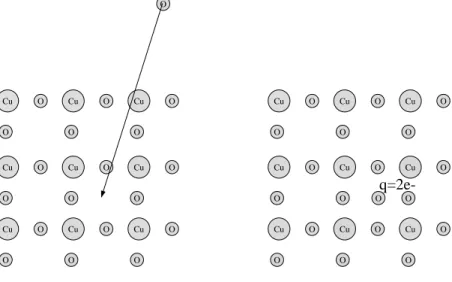
As an introduction to the effect of electronic correlations, con-sider the effect of a charged oxygen defect in one of the copper-oxygen planes of a cuprate superconductor shown in Fig. 9. Assume that the oxygen defect captures two electrons from the metallic band, going from a 2s22p4 to a 2s22p6 configuration. The defect will then become a cation, and have a net charge

Cu O O Cu O O Cu O O Cu O O Cu O O Cu O O Cu O O Cu O O Cu O O O Cu O O Cu O O Cu O O Cu O O Cu O O Cu O O Cu O O Cu O O Cu O O O

q=2e-Figure 9: A charged oxygen defect is introduced into one of the copper-oxygen planes of a cuprate superconductor. The oxygen defect captures two electrons from the metallic band, going from a 2s2_2p4 _{to a 2s}2_2p6 _{configuration.}

elec-trostatic potential and the electronic charge density will be re-duced.

If we model the electronic density of states in this material with our box-potential DOS, we can think of this reduction in the local charge density in terms of raising the DOS parabola near the defect (cf. Fig. 10). This will cause the free electronic

-eδU E_F e near charged defect Away from charged defect

Figure 10: The shift in the DOS parabola near a charged defect.

charge to flow away from the defect. Near the defect (since

e < 0 and hence eδU(r_near) < 0)

While away from the defect, δU(r_away) = 0, so n(r_away) _≈ Z₀EF D(E)DE (48) or δn(r) _≈ Z₀EF+eδU(r)D(E)DE ₋ Z₀EF D(E)DE (49) If _|eδU_{| ≪} EF, then δn(r) _≈ eδU D(EF). (50)

We can solve for the change in the electrostatic potential by solving Poisson equation.

∇2δU = 4πδρ = 4πeδn = 4πe2D(EF)δU . (51)

Let λ2 = 4πe2D(EF), then ∇2δU = λ2δU has the solution3

δU(r) = qe−

λr

r (52)

The length 1/λ = rT F is known as the Thomas-Fermi screening

length. rT F = 4πe2D(EF) −1/2 (53) 3

The solution is actuallyCe−λr/r, whereCis a constant. Cmay be deterined by lettingD(E_F) =

0, so the medium in which the charge is embedded becomes vacuum. Then the potential of the charge isq/r, soC=q.

Lets estimate this distance for our square-well model, r_{T F}2 = a0π 3(3π2_n)1/3 ≈ a0 4n1/3 rT F ≈ 1 2   n a3₀   −1/6 (54)

In Cu, for which n _≈ 1023 cm−3 (and since a0 = 0.53

◦ A) rT F Cu ≈ 1 2 1023−1/6 (0.5_× 10−8₎−1/2 ≈ 0.5 × 10 −8 _{cm = 0.5} ◦ A (55)

Thus, if we add a charge defect to Cu metal, the effect of the defect’s ionic potential is screened away for distances r > 1₂ A◦.

-e -r/r TF /r r_TF=1/4 r r_TF=1 r -e -r/r TF /r bound states free states r_TF= n-1/6

Figure 11: Screened defect potentials. As the screening length increases, states that were free, become bound.

Now consider an electron bound to an ion in Cu or some other metal. As shown in Fig. 11 the screening length decreases, and bound states rise up in energy. In a weak metal (i.e. something

like YBCO), in which the valence state is barely free, a reduction in the number of carriers (electrons) will increase the screening length, since

rT F ∼ n−1/6. (56)

This will extend the range of the potential, causing it to trap or bind more states–making the one free valance state bound.

Now imagine that instead of a single defect, we have a con-centrated system of such ions, and suppose that we decrease the density of carriers (i.e. in Si-based semiconductors, this is done by doping certain compensating dopants, or even by mod-ulating the pressure). This will in turn, increase the screening length, causing some states that were free to become bound, causing an abrupt transition from a metal to an insulator, and is believed to explain the MI transition in some transition-metal oxides, glasses, amorphous semiconductors, etc.

3.2 Fermi liquids

The purpose of these next several lectures is to introduce you to the theory of the Fermi liquid, which is, in its simplest form, a collection of Fermions in a box plus interactions.

In reality , the only physical analog is a gas of 3He, which due its nuclear spin (the nucleus has two protons, one neutron), obeys Fermi statistics for sufficiently low energies or temper-atures. In addition, simple metals, from the first or second column of the periodic table, for which we may approximate the ionic potential

V(R) = V0 (57)

are a close approximant to Fermi liquids.

Moreover, Fermi Liquid theory only describes the ”gaseous” phase of these quantum fermion systems. For example, 3He also has a superfluid (triplet), and at least in 4He-3He mixtures, a solid phase exists which is not described by Fermi Liquid The-ory. One should note; however, that the Fermi liquid theory state does serve as the starting point for the theories of

super-conductivity and super fluidity.

One may construct Fermi liquid theory either starting from a many-body diagrammatic or phenomenological viewpoint. We, as Landau, will choose the latter. Fermi liquid theory has 3 basic tenants:

1. momentum and spin remain good quantum numbers to de-scribe the (quasi) particles.

2. the interacting system may be obtained by adiabatically turning on a particle-particle interaction over some time t.

3. the resulting excitations may be described as quasi-particles with lifetimes _≫ t.

3.3 Quasi-particles

The last assumption involves a new concept, that of the quasi-particles which requires some explanation.

3.3.1 Particles and Holes

Particles and Holes are excitations of the non-interacting system at zero temperature. Consider a system of N free Fermions

each of mass m in a volume V. The eigenstates are the anti-symmetrized combinations (Slater determinants) of N different single particle states.

ψp(r) = 1

√

V e

ip_·r/¯h ₍₅₈₎

The occupation of each of these states is given bynp = θ(p−pF)

where pF is the radius of the Fermi sphere. The energy of the

system is E = X p np p2 2m (59) and pF is given by N V = 1 3π2 pF ¯ h !3 (60) Now lets add a particle to the lowest available state p = pF

then, for T = 0, µ = E0(N + 1)− E0(N) = ∂E0 ∂N = p2_F 2m . (61)

If we now excite the system, we will promote a certain number of particles across the Fermi surface SF yielding particles above

and an equal number of vacancies or holes below the Fermi surface. These are our elementary excitations, and they are

quantified by δnp = np −n0p δnp =            δ_p,p′ for a particle p′ > p_F −δ_p,p′ for a hole p′ < p_F . (62)

If we consider excitations created by thermal fluctuations, then

E_F E D(E) particle excitation hole excitation δn = -1_p δn = 1_p’

Figure 12: Particle and hole excitations of the Fermi gas.

δnp ∼ 1 only for excitations of energy within kBT of EF. The

energy of the non-interacting system is completely characterized as a functional of the occupation

E ₋ E0 = X p p2 2m(np − n 0 p) = X p p2 2mδnp. (63)

Now lets take our system and place it in contact with a par-ticle bath. Then the appropriate potential is the free energy,

E D(E) δF = p’ /2m - 2 µ δF = µ - p /2m 2 E = _F µ = p /2m 2 F δF = | µ - p /2m | 2 Figure 13: Since µ = p2

F/2m, the free energy of a particle or a hole is δF =

|p2_{/2m−µ|>0, so the system is stable to these excitations.}

which for T = 0, is F = E ₋ µN, and

F ₋ F0 = X p    p2 2m − µ   δnp. (64)

The free energy of a particle, with momentum p and δnp′ =

δp,p′ is p

2

2m − µ and it corresponds to an excitation outside SF.

The free energy of a hole δnp′ = −δp,p′ is µ− p

2

2m, which

corre-sponds to an excitation withinSF. However, since µ = p2F/2m,

the free energy of either at p = pF is zero, hence the free energy

of an excitation is p 2_/2m − µ , (65)

3.3.2 Quasiparticles and Quasiholes at T = 0

a

U

≈

e

e2

a

-a/r _TF

Figure 14: Model for a fermi liquid: a set of interacting particles an average distance a apart bound within an infinite square-well potential.

Now let’s consider a system with interacting particles an av-erage distance a apart, so that the characteristic energy of in-teraction is e_a2e−a/rT F. We will imagine that this system evolves

slowly from an ideal or noninteracting system in time t (i.e. the interaction U _≈ e_a2e−a/rT F is turned on slowly, so that the

non-interacting system evolves while remaining in the ground state into an interacting system in time t).

If the eigenstate of the ideal system is characterized by n0_p, then the interacting system eigenstate will evolve quasistatis-tically from n0_p to np. In fact if the system is isotropic and

remains in its ground state, then n0_p = np. However, clearly in

some situations (superconductivity, magnetism) we will neglect some eigenstates of the interacting system in this way.

Now let’s add a particle of momentumpto the non-interacting ideal system, and slowly turn on the interaction. As U is

p time = 0 U = 0 p p time = t U = (e /a) exp(-a/r )2 TF

Figure 15: We add a particle with momentum pto our noninteracting (U = 0) Fermi liquid at time t= 0, and slowly increase the interaction to its full value U at time t. As the particle and system evolve, the particle becomes dressed by interactions with the system (shown as a shaded ellipse) which changes the effective mass but not the momentum of this single-particle excitation (now called a quasi-particle).

switched on, we slowly begin to perturb the particles close to the additional particle, so the particle becomes dressed by these interactions. However since momentum is conserved, we have created an excitation (particle and its cloud) of momentum p. We call this particle and cloud a quasiparticle. In the same way,

if we had introduced a hole of momentum p below the Fermi surface, and slowly turned on the interaction, we would have produced a quasihole.

Note that this adiabatic switching on procedure will have difficulties if the lifetime of the quasi-particle τ < t. If so, then the the quasiparticle could decay into a number of other quasiparticles and quasiholes. If we shorten t so that again

τ _≫ t, then switching on U could excite the system out of its ground state). We will show that such difficulties do not arise so long as the energy of the particle is close to the Fermi energy. Here there are few states accessible for creating particle-hole excitations so collisions are rare.

To estimate this lifetime consider the following argument from AGD: A particle with momentum p₁ above the Fermi surface (p1 > pF) interacts with one of the particles below the

Fermi surface with momentum p₂. As a result, two new par-ticles appear above the Fermi surface (all other states are full) with momenta p₃ and p₄. This may also be interpreted as a particle of momentum p₁ decaying into particles with momenta

p

p

p

p

Figure 16: A particle with momentum p1 above the Fermi surface (p1 > pF) interacts

with one of the particles below the Fermi surface with momentump2. As a result, two

new particles appear above the Fermi surface (all other states are full) with momenta

p₃ and p₄..

p₃ and p₄ and a hole with momentum p₂. By Fermi’s golden rule, the total probability of such a process if proportional to

1 τ ∝ Z δ (ε1 +ε2 − ε3 − ε4)d3p2d3p3 (66) where ε1 = p 2 1

2m − EF, and the integral is subject to the

con-straints of energy and momentum conservation and that

p2 < pF , p3 > pF , p4 = |p1 +p2 − p3| > pF (67)

It must be that ε1 + ε2 = ε3 + ε4 > 0 since both particles 3

if ε1 is small, then |ε2| ∼< ε1 is also small, so only of order

ε1/EF states may scatter with the state k1, conserve energy,

and obey the Pauli principle. Thus, restricting ε2 to a narrow

shell of width ε1/EF near the Fermi surface, and reducing the

scattering probability 1/τ by the same factor.

k 1 k 4 E_F 3 2 1 4 k - k₁ 3 k - k₄ 2 E N(E) k_y k_x k 3 k 2

Figure 17: A quasiparticle of momentum p1 decays via a particle-hole excitation

into a quasiparticle of momentum p₄. This may also be interpreted as a particle of momentum p1 decaying into particles with momenta p3 and p4 and a hole with

momentum p2. Energy conservation requires |ε2| _∼< ε1. Thus, restricting ε2 to a

narrow shell of width ε1/EF near the Fermi surface. Momentum conservation k1−

k3 = k4−k2 further restricts the available states by a factor of about ε1/EF. Thus

the lifetime of a quasiparticle is proportional to ε1

EF

₋2

.

momentum conservation

k_{1 −}k₃ = k_{4 −} k₂. (68)

Since ε1 and ε2 are confined to a narrow shell around the Fermi

surface, so too are ε3 and ε4. This can be seen in Fig. 17, where

the requirement that k_{1 −} k₃ = k_{4 −} k₂ limits the allowed states for particles 3 and 4. If we take k₁ fixed, then the allowed states for 2 and 3 are obtained by rotating the vectorsk₁₋k₃ =

k₄₋k₂; however, this rotation is severely limited by the fact that particle 3 must remain above, and particle 2 below, the Fermi surface. This restriction on the final states further reduces the scattering probability by a factor of ε1/EF.

Thus, the scattering rate 1/τ is proportional to ε1

E_F

2

so that excitations of sufficiently small energy will always be sufficiently long lived to satisfy the constraints of reversibility. Finally, the fact that the quasiparticle only interacts with a small number of other particles due to Thomas-Fermi screening (i.e. those within a distance _≈ rT F), also significantly reduces the scattering rate.

3.4 Energy of Quasiparticles.

As in the non-interacting system, excitations will be quanti-fied by the deviation of the occupation from the ground state occupation n0_p

δnp = np − n0_p. (69) At low temperatures δnp ∼ 1 only for p ≈ pF where the

par-ticles are sufficiently long lived that τ _≫ t. It is important to emphasize that only δnp not n0_p or np, will be physically rele-vant. This is important since it does not make much sense to talk about quasiparticle states, described by np, far from the Fermi surface since they are not stable.

For the ideal system

E ₋ E0 =

X

p

p2

2mδnp . (70)

For the interacting system E[np] becomes much more compli-cated. If however δnp is small (so that the system is close to its ground state) then we may expand:

E[np] = Eo +

X

p ǫpδnp + O(δn

2

where ǫp = δE/δnp. Note that ǫp is intensive (ie. it is indepen-dent of the system volume). If δnp = δp,p′, then E ≈ E0+ǫp′; i.e., the energy of the quasiparticle of momentum p′ is ǫp′.

In practice we will only need ǫp near the Fermi surface where

δnp is finite. So we may approximate

ǫp ≈ µ + (p− pF) · ∇p ǫp|_p

F (72)

where _∇pǫp = vp, the group velocity of the quasiparticle. The ground state of the N + 1 particle system is obtained by adding a particle withǫp = ǫF = µ = ∂E_∂N0 (at zero temperature); which

defines the chemical potential µ. We make learn more about

ǫp by employing the symmetries of our system. If we explicitly display the spin-dependence,

ǫp,σ = ǫ₋p,₋σ under time-reversal (73)

ǫp,σ = ǫ₋p,σ under BZ reflection (74)

So ǫp,σ = ǫ₋p,σ = ǫp,₋σ; i.e. in the absence of an external

magnetic field, ǫp,σ does not depend upon σ if. Furthermore,

for an isotropic system ǫp depends only upon the magnitude of

p, _|p_|, so p and vp = ∇ǫp(|p|) = _|p_p|dǫp(| p_|)

define m∗ as the constant of proportionality at the fermi surface

vp_F = pF/m∗ (75)

Using m∗ it is useful to define the density of states at the fermi surface. Recall, that in the non-interacting system,

D(EF) = 1 2π2   2m ¯ h2   3/2 E_F1/2 = mpF πh¯3 (76) where p = ¯hk, and E = p2/2m. Thus, for the interacting system at the Fermi surface

Dinteracting(EF) =

m∗pF

πh¯3 , (77)

where the m∗ (generally > m, but not always) accounts for the fact that the quasiparticle may be viewed as a dressed particle, and must “drag” this dressing along with it. I.e., the effective mass to some extent accounts for the interaction between the particles.

4 Interactions between Particles: Landau Fermi Liquid

4.1 The free energy, and interparticle interactions

The thermodynamics of the system depends upon the free en-ergy F, which at zero temperature is

F ₋F0 = E − E0 − µ(N − N0). (78)

Since our quasiparticles are formed by adiabatically switching on the interaction in the N + 1 particle ideal system, adding one quasiparticle to the system adds one real particle. Thus,

N ₋ N0 = X p δnp, (79) and since E ₋ E0 ≈ X p ǫpδnp, (80) we get F ₋ F0 ≈ X p (ǫp − µ)δnp. (81) As shown in Fig. 18, we will be interested in excitations of the system which distort the Fermi surface by an amount propor-tional to δ. For our theory/expansion to remain valid, we must

δ

Figure 18: We consider small distortions of the fermi surface, proportional to δ, so that 1 N P p|δnp| ≪1. have 1 N X p |δnp| ≪ 1. (82) Where δnp 6= 0, ǫp −µ will also be of order δ. Thus,

X

p (ǫp −µ)δnp ∼ O(δ

2_{), (83)}

so, to be consistent we must add the next term in the Taylor series expansion of the energy to the expression for the free energy. F ₋F0 = X p (ǫp − µ)δnp + 1 2 X p,p′ fp,p′δnpδnp′ + O(δ3) (84)

where

fp,p′ =

δE δnpδnp′

(85)

The term, proportional to fp,p′, was added (to the Sommerfeld theory) by L.D. Landau. Since each sum over p is proportional to the volumeV, as isF, it must be thatfp,p′ ∼ 1/V . However, it is also clear thatfp,p′ is an interaction between quasiparticles, each of which is spread out over the whole volume V , so the probability that they will interact is _∼ r_{T F}3 /V , thus

fp,p′ ∼ r_{T F}3 /V 2 (86) In general, since δnp is only of order one near the Fermi surface, we will only care about fp,p′ on the Fermi surface (as-suming that it is continuous and changes slowly as we cross the Fermi surface. Interested in fp,p′ ǫp=ǫ_p′=µ in only! (87)

Thus, fp,p′ only depends upon the angle between p and p′. We can also reduce the spin dependence of fp,p′ to a symmet-ric and anti symmetsymmet-ric part. First in the absence of an external

field, the system should be invariant under time-reversal, so

fpσ,p′σ′ = f₋p₋σ,₋p′₋σ′ , (88)

and, in a system with reflection symmetry

fpσ,p′σ′ = f₋pσ,₋p′σ′ . (89)

Then

fpσ,p′σ′ = fp₋σ,p′₋σ′ . (90)

It must be then that f depends only upon the relative orienta-tions of the spins σ and σ′, so there are only two independent components fp_↑,p′_↑ and fp_↑,p′_↓. We can split these into sym-metric and antisymsym-metric parts.

f_pa_,p′ = 1 2 fp_↑,p′_↑ −fp_↑,p′_↓ f_ps_,p′ = 1 2 fp_↑,p′_↑ +fp_↑,p′_↓ . (91)

f_pa_,p′ may be interpreted as an exchange interaction, or

fpσ,p′σ′ = fps,p′ +σ · σ′fpa,p′ (92) where σ and σ′ are the Pauli matrices for the spins.

Our ideal system is isotropic in momentum. Thus, f_pa_,p′ and

so we may expand either f_pa_,p′ and f_ps_,p′ f_pα_,p′ = ∞ X l=0f α l Pl(cosθ). (93)

Conventionally these f parameters are expressed in terms of reduced units. D(EF)flα = V m∗pF π2_h¯3 f α l = Flα. (94)

4.2 Local Energy of a Quasiparticle

p

Figure 19: The addition of another particle to a homogeneous system will yeilds in forces on the quasiparticle which tend to restore equilibrium.

Now consider an interacting system with a certain distribu-tion of excited quasiparticles δnp′. To this, add another quasi-particle of momentum p (δn′_{p →} δn′_p+δp,p′). From Eq. 84 the

free energy of the additional quasiparticle is ˜ ǫp −µ = ǫp − µ + X p′ fp′,pδnp′ , (95) (recall that fp,p′ = fp′,p). Both terms here are O(δ). The

second term describes the free energy of a quasiparticle due to the other quasiparticles in the system (some sort of Hartree-like term).

The term ˜ǫp plays the part of the local energy of a

quasi-particle. For example, the gradient of ˜ǫp is the force the system exerts on the additional quasiparticle. When the quasiparticle is added to the system, the system is inhomogeneous so that

δnp′ = δnp′(r). The system will react to this inhomogeneity by minimizing its free energy so that _∇rF = 0. However, only

the additional free energy due the added particle (Eq. 95) is inhomogeneous, and has a non-zero gradient. Thus, the system will exert a force

−∇rǫ˜= −∇r

X

p′

fp′,pδnp′(r) (96) on the added quasiparticle resulting from interactions with other quasiparticles.

4.2.1 Equilibrium Distribution of Quasiparticles at Finite T

˜

ǫp also plays an important role in the finite-temperature prop-erties of the system. If we write

E ₋ E0 = X p ǫpδnp + 1 2 X p,p′ fp′,pδnp′δnp (97) Now suppose that P

p |hδnpi| ≪ N, as needed for the expansion above to be valid, so that

δnp = hδnpi + (δnp − hδnpi) (98) where the first term is _O(δ), and the second _O(δ2). Thus,

δnpδnp′ ≈ −hδnpihδnp′i+ hδnpiδnp′ +hδnp′iδnp (99) We may use this to rewrite the energy of our interacting system

E ₋E0 ≈ X p ǫpδnp − 1 2 X p,p′ fp′,phδnpihδnp′i + X p,p′ fp′,phδnpiδnp′ ≈ X p   ǫp + X p′ fp′,phδnp′i   δnp − 1 2 X p,p′ fp′,phδnpihδnp′i ≈ X phǫ˜piδnp − 1 2 X p,p′ fp′,phδnpihδnp′i +O(δ4) (100) At this point, we may repeat the arguments made earlier to de-termine the fermion occupation probability for non-interacting

Fermions (the constant factor on the right hand-side has no effect). We will obtain

np(T, µ) = 1 1 + expβ(_hǫ˜pi − µ) , (101) or δnp(T, µ) = 1 1 + expβ(_hǫ˜pi − µ) − θ(pf − p). (102)

However, at least for an isotropic system, this expression bears closer investigation. Here, the molecular field (evaluated within

kBT of the Fermi surface)

hǫ˜p − ǫpi =

X

p′

fp′,phδnp′i (103) must be independent of the location of p on the Fermi sur-face (and of course, spin), and is thus constant. To see this, reconsider the Legendre polynomial expansion discussed earlier

hǫ˜p − ǫpi = X p′ fp′,phδnp′i ∝ X l Z d3pflPl(cosθ)hδnp′i ∝ f0 Z d3p_hδnp′i = 0 (104)

In going from the second to the third line above, we made use of the isotropy of the system, so that _hδnp′i is independent of the angle θ. The evaluation in the third line, follows from particle number conservation. Thus, to lowest order in δ

np(T, µ) = 1

1 + expβ(ǫp − µ)

+_O(δ4) (105) 4.2.2 Local Equilibrium Distribution

Now suppose we introduce a local weak perturbation such as the type discussed in Sec. 4.2 to an isotropic system at zero temperature. Such a perturbation could be caused by, eg. a sound wave or a weak magnetic field (which you will explore in your homework, to calculate the sound velocity and suscepti-bility of a Landau Fermi liquid). This pertubation will cause a small deviation of the equilibrium distribution function, leading to a new ”local equilibrium” distribution

¯

np = np(˜ǫp − µ) (106) where the argument of the RHS indicates that this is the distri-bution corresponding to the local energy discussed above. The

gradient of the local energy yields a force which tries to restore the equilibrium distribution np(ǫp − µ) derived above). The deviation from true equilibrium is

δnp = np − n¯p (107) = δn¯p +

∂np(ǫp − µ)

∂ǫp

(˜ǫp − ǫp) (108) Using Eq. 95, we find

δnp = δn¯p − ∂np ∂ǫp X p′ fp,p′δnp′ (109) At zero temperature, the factor ∂np

∂ǫp = −δ(ǫp−µ), so both δnp

and δn¯p are restricted to the fermi surface. Since the pertuba-tion of interest is small, we may expand both δnp and δn¯p in a series of Legendre polynomials, and we will also split them into symmetric and antisymmetric parts (as we did with fp,p′ previously). For example,

δns_p = X

l δ(ǫp −µ)δn s

lPl (110)

If we make a similar expansion for the antisymmetric and sym-metric parts of δn¯p, and substitute this back into Eq. 108, then

we find δn¯a_l =  1 + F_la 2l + 1  δna l (111) δn¯s_l =  1 + F_ls 2l + 1  δns l (112)

4.3 Effective Mass m∗ of Quasiparticles

This argument most closely follows that of AGD, and we will follow their notation as closely as possible (without introducing any new symbols). In particular, since an integration by parts is necessary, we will use a momentum integral (as opposed to a momentum sum) notation

X

p → V

Z d3p

(2πh¯)3 . (113)

The net momentum of the volume V of quasiparticles is

P_qp = 2V Z d

3_p

(2πh¯)3pnp net quasiparticle momentum (114)

which is also the momentum of the Fermi liquid. On the other hand since the number of particles equals the number of quasi-particles, the quasiparticle and particle currents must also be

equal

J_qp = J_p = 2V Z d

3_p

(2πh¯)3vpnp net quasiparticle and particle current

(115) or, since the momentum is just the particle mass times this current

P_p = 2V mZ d

3_p

(2πh¯)3vpnp net quasiparticle and particle current

(116) where v_p = _∇pǫ˜p, is the velocity of the quasiparticle. So

Z d3p

(2πh¯)3pnp = m

Z d3p

(2πh¯)3∇pǫ˜pnp (117)

Now make an arbitrary change of np and recall that ˜ǫp depends upon np, so that δ˜ǫp = V X σ′ Z d3p (2πh¯)3fp,p′δnp′ . (118)

For Eq. 117, this means that

Z d3p (2πh¯)3pδnp = m Z d3p (2πh¯)3∇pǫ˜pδnp (119) +mV Z d 3_p (2πh¯)3 X σ′ Z d3p′ (2πh¯)3∇p fp,p′δnp′ np,

or integrating by parts (and renaming p _→ p′ in the last part), we get Z d3p (2πh¯)3 p mδnp = Z d3p (2πh¯)3∇p˜ǫpδnp (120) −V X σ′ Z d3p′ (2πh¯)3 Z d3p (2πh¯)3δnpfp,p′∇p′np′ ,

Then, since δnp is arbitrary, it must be that the integrands themselves are equal

p m = ∇pǫ˜p − X σ′ V Z d 3_p′ (2πh¯)3fp,p′∇p′np′ (121) The factor _∇p′np′ = −p ′

p′δ(p′ −pF). The integral may be

eval-uated by taking advantage of the system isotropy, and setting

p parallel to the z-axis, since we mostly interested in the prop-erties of the system on the Fermi surface we take p = pF, let θ

be the angle between p (or the z-axis) and p′, and finally note that on the Fermi surface

∇p˜ǫp|p=p_F = vF = pF/m ∗_{. Thus,} pF m = pF m∗ + X σ′ Z p′2dpdΩ (2πh¯)3 fpσ,p′σ′ p′ p′δ(p′ −pF) (122)

However, since both p and p′ are restricted to the Fermi surface p′

p′ = cosθ, and evaluating the integral over p, we get

1 m = 1 m∗ + V pF 2 X σ,σ′ Z dΩ (2πh¯)3fpσ,p′σ′ cosθ , (123)

where the additional factor of 1₂ compensates for the additional spin sum. If we now sum over both spins, σ and σ′, only the symmetric part of f survives (the sum yields 4fs), so

1 m = 1 m∗ + 4πV pF (2πh¯)3 Z d(cosθ)fs(θ) cosθ , (124)

We now expand f in a Legendre polynomial series

fα(θ) = X

l f α

l Pl(cosθ), (125)

and recall that P0(x) = 1, P1(x) = x, .... that

Z 1

−1dxPn(x)Pm(x)dx =

2

2n+ 1δnm (126) and finally that

D(0)f_lα = V m∗pF π2_h¯3 f α l = Flα , (127) we find that 1 m = 1 m∗ + F₁s 3m∗ , (128)

Quantity Fermi Liquid Fermi Liquid/Fermi Gas Specific Heat Cv = m ∗_p F 3¯h3 k 2 BT _CC_VV₀ = m ∗ m = 1 + F1s/3 Compressibility _κκ 0 = 1+F₀s 1+F₀s/3 Sound Velocity c2 = p2F 3mm∗ (1 + F0s) c c₀ 2 = 1+F0s 1+F₁s/3 Spin Susceptibility χ = m∗pF π2¯h3 β2 1+F₀a χ χ₀ = 1+F₁s/3 1+F₀a Table 1: Fermi Liquid relations between the Landau parameters Fα

n and some

exper-imentally measurable quantities. For the latter, a zero subscript indicates the value for the non-interacting Fermi gas.

or m∗/m = 1 + F₁s/3.

The effective mass cannot be experimentally measured di-rectly; however, it appears in many physically relevant measur-able quantities, including the specific heat

CV =    ∂E/V ∂T    V N = 1 V ∂ ∂T X p ǫ˜pnp. (129) To lowest order in δ, we may neglect fp,p′ in both ˜ǫp and np, so CV = 1 V X p ǫp ∂np ∂T . (130)

Recall that the density of statesD(E) = P

pδ(E−ǫp), and

system, that _∂T∂µ is negligible, we get, CV = 1 V Z dǫD(ǫ)ǫ ∂ ∂T 1 expβ(ǫ ₋ µ) + 1 . (131) This integral is identical to the one we had to evaluate for the non-interacting system, and yields the result

CV = π2 3V k 2 BT D(EF) = k 2 BT m∗pF 3¯h3 . (132)

Thus, measuring the electronic contribution to the specific heat

CV yields information about the effective mass m∗, and hence

F₁s. Other measurements are related to some of the remaining Landau parameters, as summarized in table 1.