Variable Neighbourhood Decomposition Search for 0-1
Mixed Integer Programs
Jasmina Lazi´ca, Sa¨ıd Hanafi∗,b, Nenad Mladenovi´ca, Dragan Uroˇsevi´cc aBrunel University, West London UB8 3PH, UK
bLAMIH - Universite de Valenciennes,
ISTV 2 Le Mont Houy, 59313 Valenciennes Cedex 9, France cMathematical Institute, Serbian Academy of Sciences and Arts,
Kneza Mihaila 36, 11000 Belgrade, Serbia
Abstract
In this paper we propose a new hybrid heuristic for solving 0-1 mixed integer pro-grams based on the principle of variable neighbourhood decomposition search. It combines variable neighbourhood search with a general-purpose CPLEX MIP solver. We perform systematic hard variable fixing (or diving) following the vari-able neighbourhood search rules. The varivari-ables to be fixed are chosen accord-ing to their distance from the correspondaccord-ing linear relaxation solution values. If there is an improvement, variable neighbourhood descent branching is per-formed as the local search in the whole solution space. Numerical experiments have proven that exploiting boundary effects in this way considerably improves solution quality. With our approach, we have managed to improve the best known published results for 8 out of 29 instances from a well-known class of very difficult MIP problems. Moreover, computational results show that our method outperforms the CPLEX MIP solver, as well as three other recent most successful MIP solution methods.
Key words: 0-1 mixed integer programming, Metaheuristics, Variable neighbourhood search, CPLEX.
1. Introduction
The 0-1 mixed integer programming (0-1 MIP) problem consists of maximis-ing or minimismaximis-ing a linear function, subject to equality or inequality constraints and binary choice restrictions on some of the variables. The 0-1 mixed integer programming problem (P) can be expressed as:
∗Corresponding author. Fax: +33 327511940
(P) minPnj=1cjxj s.t. Pnj=1aijxj ≥bi ∀i∈M ={1,2, . . . , m} xj∈ {0,1} ∀j∈ B 6=∅ xj≥0 ∀j∈ C
where the set of indices{1,2, . . . , n}of variables is partitioned into two subsets B = {1,2, . . . , p} and C = {p+ 1, p+ 2, . . . , n}, corresponding to binary and continuous variables, respectively, withp∈N, 1≤p≤n. We will also use the following short form notation for problemP:
(P) min{cTx|x∈X} (1)
where X = {x ∈ Rn | Ax ≥ b, x
j ∈ {0,1} for j = 1, . . . , p, xj ≥ 0 for j = p+ 1, . . . , n}.
Numerous combinatorial optimisation problems, including a wide range of practical problems in business, engineering and science can be modelled as 0-1 MIP problems (see [1]). Several special cases of the 0-1 MIP problem, such as knapsack, set packing, cutting and packing, network design, protein alignment, travelling salesman and some other routing problems, are known to be NP-hard [2]. Complexity results prove that the computational resources required to op-timally solve some 0-1 MIP problem instances can grow exponentially with the size of the problem instance. Over several decades many contributions have led to successive improvements in exact methods such as branch-and-bound and branch-and-cut, branch-and-price, dynamic programming, Lagrangian re-laxation, and linear programming. However, many MIP problems still cannot be solved within acceptable time and/or space limits by the best current exact methods. As a consequence, metaheuristics have attracted attention as possible alternatives or supplements to the more classical approaches. Although exact methods can successfully solve to optimality problems with small dimensions (see, for instance, [3]), for large-scale problems they cannot find an optimal so-lution with reasonable computational effort, hence the need to find near-optimal solutions. It is well known that heuristics and relaxations are useful for providing upper and lower bounds of the optimal value for large and difficult optimisation problems. Several hybrid methods for solving 0-1 MIP problems have been pro-posed recently, mainly those combining heuristics and exact methods ([4, 5, 6], [7, 8, 9], [10, 11, 12], [13]).
In this paper we propose a new hybrid approach for solving 0-1 MIP, which combines the variable neighbourhood decomposition search (VNDS) with an exact solution method.
We first find an initial feasible solution and an optimal solution of the LP-relaxation of the problem, using the CPLEX solver. Those solutions generate the initial lower and upper bounds. Trivially, if the LP-solution is 0-1 MIP feasible, we stop the search. Otherwise, at each iteration, we rank variables in the non-decreasing order of their absolute values of the difference between the LP-solution and the incumbent solution values. Subproblems within VNDS are obtained by successively fixing a certain number of variables in the order
provided. In this way, the subproblem involves the free variables which are furthest from their linear relaxation values. Then these subproblems are solved exactly or within the CPU time limit. The subproblems are changed by the hard fixing of the variables (or diving), according to VNS rules.
This paper is organised as follows. In Sec. 2, we provide the necessary mathematical definitions and notations and a brief overview of the existing approaches related to our work. In Sec. 3, we describe VNDS heuristic. In Sec. 4, we provide a detailed description of our VNDS implementation for solving 0-1 MIP problems. Next, in Sec. 5, we analyse the performance of the VNDS method as compared to the other three methods mentioned and to the CPLEX solver alone. Last, in Sec. 6, we give some final remarks and conclusions.
2. Preliminaries
In this section, we first present the mathematical notations and a survey of the closely related recent work.
2.1. Notations and definitions
To formally describe the process of hard variable fixing [14], we introduce the notion of a reduced problem, which is obtained from the original problem by assigning given values to some variables. Formally, let x0 be an arbitrary vector of binary values,x0
j ∈ {0,1} forj∈ B, andJ ⊆ Ban arbitrary subset of binary variable indices. The reduced problem associated withx0and J can be defined as follows: P(x0, J) min cTx s.t. Ax≥b xj =x0j ∀j∈J xj ∈ {0,1} ∀j∈ B 6=∅ xj ≥0 ∀j∈ C (2)
Obviously,P(x0,∅) =P andν(P(x0, J))≤ν(P(x0, J0)), for any setsJ andJ0,
such thatJ⊆J0⊆ B, whereν(P) is the optimal objective function value of the
optimisation problemP.
The LP-relaxation of problem P which results from dropping the integer requirement onx, is denoted as LP(P), i.e. :
LP(P) min cTx s.t. Ax≥b xj∈[0,1] ∀j∈ B 6=∅ xj≥0 ∀j∈ C
Given two solutionsx andy of the problemP and a subset of indicesJ ⊆ B, we define the distance betweenxandy as:
δ(J, x, y) =X j∈J
More generally, if ¯x is an optimal solution of the LP relaxation LP(P) (not necessarily MIP feasible), the distance betweenxand xcan be defined in the same way, for the subsetJ of the indices of variables which are integer feasible inx.
LetXbe the solution space of the problem P considered. The neighbourhood structures{Nk |k=kmin, . . . , kmax}, 1≤kmin ≤kmax≤| B |, can be defined if the distanceδ(B, x, y) between any two solutionsx, y∈X is known. The set of all solutions in thekth neighbourhood of x∈X is denoted asNk(x), where
Nk(x) ={y∈X|δ(B, x, y) ≤ k}.
From the definition of Nk(x), it follows that Nk(x) ⊂ Nk+1(x), for any k ∈ {kmin, kmin+ 1, . . . , kmax−1}, sinceδ(B, x, y) ≤ kimpliesδ(B, x, y) ≤ k+ 1. It is trivial that, if we completely explore neighbourhood Nk+1(x), it is not necessary to explore neighbourhoodNk(x).
2.2. Local branching
Local branching (LB) was introduced by Fischetti and Lodi in 2003 [6], as a branching strategy for MIP problems which can also be effectively used as a heuristic for improving the incumbent solution. The usage of local branching as an improvement heuristic relies on the observation that the neighbourhood of a feasible 0-1 MIP solution (in terms of the rectangular distance) often contains better solutions. More precisely, letx0 be the incumbent solution,x∗ the best
known solution found andε > 0 a small non-negative real number. The local branching heuristic solves the following subproblem:
P(k, x0) min cTx s.t. Ax≥b δ(B, x, x0)≤k cTx≤cTx∗−ε xj∈ {0,1} ∀j∈ B 6=∅ xj≥0 ∀j∈ C
Local branching combines local search with a generic MIP solver, which is used as a black box for exactly solving problemsP(k, x0) in an iterative process.
After the first feasible solution x0 is found (if it exists), the first subproblem
P(k, x0), fork=kmin, is solved (wherek
min ∈Nis a parameter which defines the minimum neighbourhood size). Then, if an improved solution is found, a new subproblem is derived and solved; this is repeated as long as an improvement can be made in the objective function value. This basic mechanism is extended by introducing time limits, automatically modifying the neighbourhood sizek and adding diversification strategies in order to improve the performance. 2.3. Variable neighbourhood search branching
Variable neighbourhood search (VNS) is a metaheuristic which is based on the systematic change of neighbourhoods towards the local optima and also
out of the regions which contain them [15, 16]. The pseudo-code of the step which performs systematic change is given in Fig. 1. In this figure,x, x0 and
k denote the incumbent solution, new solution and the neighbourhood index, respectively.
Procedure NeighbourhoodChange(x, x0, k)
1 ifcTx0< cTxthen
2 x←x0,k←1; //Make a move.
3 elsek←k+ 1; //Next neighbourhood. Figure 1: Neighbourhood change pseudo-code.
VNS branching (VNSB) is a heuristic for solving MIP problems, using the general-purpose MIP solver CPLEX as a black-box [8]. VNSB adds constraints to the original problem, as in the LB method. However, in VNSB, neighbour-hoods are changed in a systematic manner, according to the rules of the general VNS algorithm [16]. The main idea of both LB and VNSB for solving MIP is in fact a change of the neighbourhood during the search. Therefore, LB can be seen as a specialised variant of VNSB (or vice versa): (i) in LB the local search step is performed in the neighbourhood of the fixed size k > 1 (wherek is a given parameter), instead ofk=1; (ii) as a consequence of (i), backwardinstead of forward VNS (see [17]) is used in the inner loop (i.e., instead of increasing neighbourhood by 1 in the intensification step, its current size, initially set at k, is reduced by half); (iii) the shaking step of VNS and the diversification step of LB differ only in the area from which a random feasible solution is chosen. In LB the area is a disk with radii 1 andk+dv·[k
2] where dv is the current number of diversifications (see [6] for details), while in VNSB the disk is defined by radiikcurandkcur+kstep, wherekcurdefines the current neighbourhood size andkstep is a given parameter.
Variable neighbourhood descent(VND) is a variant of VNS in which neigh-bourhoods are changed deterministically. Starting from the first feasible solu-tion, the current neighbourhood of the current incumbent solution x is com-pletely explored and if a better solutionx0 is found, then the whole process is
iterated, starting fromx0 as the current incumbent; otherwise, the next
neigh-bourhood ofxis explored. The whole process is iterated until a maximal number of neighbourhoods is reached, or the predefined time limit is exceeded.
Both VNSB and the approach presented within this paper use the im-plementation of VND with only a time limit as a stopping criterion. The pseudo-code for the VND procedure is given in Fig. 2, where the statement y = LocalSearch(P, x) means that some local search technique is applied to the problem P, starting from x as the initial solution, with solution y as a result.
Procedure VND(P, x, tvnd) 1 repeat
2 k= 1; tstart=cpuT ime( ); 3 repeat
4 x0 =LocalSearch(P(k, x), x); //Find the best neighbour in N
k(x). 5 NeighbourhoodChange(x, x0, k); //Change neighbourhood.
6 tend=cpuT ime( ),t=tend−tstart; 7 untilcTx0=cTxort > tvnd;
8 untilt > tvnd; 9 returnx0.
Figure 2: VND pseudo-code.
2.4. Relaxation induced neighbourhood search
The relaxation induced neighbourhoods search (RINS for short), proposed by Danna et al. in 2005 (see [7]), solves reduced problems at some nodes of a branch-and-bound tree when performing a tree search. It is based on the observation that often an optimal solution of a 0-1 MIP and an optimal solution of its LP relaxation have some variables with the same values. Therefore, it is more likely that some variables in the incumbent integer feasible solution which have the same value as the corresponding variables in the linear relaxation solution, will have the same value in the optimal solution. Hence, it seems justifiable to fix the values of those variables and then solve the remaining subproblem, in order to obtain a 0-1 MIP feasible solution with a good objective value. On the basis of this idea, at a node of the branch-and-bound tree, the RINS heuristic performs the following procedure: (i) fix the values of the variables which are the same in the current continuous relaxation and the incumbent integral solution; (ii) set the objective cutoff to the value of the current incumbent solution; and (iii) solve the MIP subproblem on the remaining variables.
More precisely, let x0 be the current incumbent feasible solution, ¯xthe so-lution of the continuous relaxation at the current node,J ={j∈ B |x0
j = ¯xj}, x∗ the best known solution found andε > 0 a small nonnegative real number.
Then RINS solves the following reduced problem:
P(x0, x∗, J) min cTx s.t. Ax≥b xj=x0j ∀j∈J cTx≤cTx∗−ε xj∈ {0,1} ∀j∈ B 6=∅ xj≥0 ∀j∈ C
Since solving MIP problems optimally can be time consuming, it is desirable to avoid solving reduced problems which are very similar. For example, if the LP relaxations are very similar, adjacent nodes of the branch-and-bound tree tend to have very similar optimal solutions. Therefore, one way to meet this difficulty would be to solve reduced problems only if a new best solution x∗
was found during the process. Hence, with this strategy, RINS provides more diversification than local branching because the optimal LP solution potentially changes at far nodes (nodes which are far with respect to the path length from the root node of the branch-and-bound tree). Experiments have shown that the RINS heuristic thus described gives the best results if not applied to each node of the branch-and-bound tree, but with a certain frequencyf >>1 (usuallyf = 100). Another way to meet the possibility of taking a long computational time to find the MIP optimal solution is to limit the time for solving subproblems. 2.5. Other Approaches
Recently, a few similar approaches have emerged which follow the idea of decomposition based on successive approximations. Although some of them are problem specific, their ideas can easily be extended to solve general MIP problems.
One idea for generating and exploiting small subproblems within a successive approximations method was proposed by Glover ([18, 19]), but without any empirical evidence.
Hanafi and Wilbaut have introduced several enhanced versions ([10, 9, 11]) of the exact algorithm proposed by Soyster in [3]. The process consists in generating two sequences of upper and lower bounds until the optimality of the problem solution is proven. This process is used as a heuristic with a maximum number of iterations. The integration of mixed integer programming relaxations allows the lower bounds to be refined and diversifies the search. They have also suggested a new proof of the finite convergence of this algorithm. In addition, they have proposed a new two-phase heuristic algorithm which uses dominance properties to decrease the number of reduced problems to be solved exactly. The proposed heuristics have been tested on the multidimensional knapsack problem. The results obtained on a set of available and difficult instances show the efficiency of this method.
Mitrovi´c-Mini´c and Punnen have developed a very large scale variable bourhood search (VLSVNS) (see [12]), based on the very large scale neigh-bourhood search (see [5]) and VNS ([16]). This approach uses the exponential k-exchange neighbourhoods with large values for k. These very large neigh-bourhoods are then explored by exactly or approximately solving the sequence of subproblems. The size of each subproblem and the CPU time allowed for solving it are increased in the VNS manner. VLSVNS has been applied effi-ciently for solving the general assignment problem and it outperforms existing methods ([12]).
3. Variable neighbourhood decomposition search
Variable neighbourhood decomposition search (VNDS) is a two-level VNS scheme for solving optimisation problems, based upon the decomposition of the problem [20]. In general, an optimisation problem can be defined as
where f, x, X and S are the real valued objective function, feasible solution, feasible set, and solution space, respectively. Note that MIP problem defined in (1) is a special case of optimisation problem, withf(x) =cTxandS=Rn. We will denote withAthe set of all solution attributes (or variable indices, if setX is enumerable) and withx(J) = (xj)j∈J the subvector associated with the set of solution attributes (or variable indices) J ⊆ A and solution x. The notion of a reduced problem, defined in (2), can be generalised for any optimisation problem P. Namely, if P is a given optimisation problem, then the reduced problem P(x0, J), associated with the arbitrary feasible solution x0 and the subset of solution attributesJ ⊆ A, can be defined as:
P(x0, J) min{f(x)|x∈X, X⊆S, x
j=x0j,∀j∈J}.
The steps of VNDS method are presented in Fig. 3, where the statement y=LocalSearch(P, x, t) means that a local search technique is applied to the problem P, starting fromx as the initial solution, with a given running time limitt and with solutiony as a result.
Procedure VNDS(P, x, kmin, kmax, tmax, tsub, tvnd) 1 repeat
2 k=kmin; tstart=cpuT ime( ); 3 repeat
4 Choose randomlyJk ⊆ Asuch that|Jk |=k;
5 x0(J k) =x(Jk);Jk=A \Jk; 6 x0(Jk) =LocalSearch(P(x, Jk), x(Jk), tsub); 7 ifcTx0< cTx 8 thenx00=VND(P, x0, tvnd); 9 else x00=x0; 10 NeighbourhoodChange(x, x00, k);
11 tend=cpuT ime( );t=tend−tstart; 12 until(k=kmax)or(t > tmax); 13 untilt > tmax;
14 returnx00;
Figure 3: VNDS pseudo-code.
Input parameters for the VNDS algorithm are the optimisation problemP, the initial solutionx, minimal numberkmin of neighbourhoods to be explored, maximal numberkmaxof neighbourhoods to be explored, maximal running time allowed tmax, time allowed for the inner local search procedure tsub and time allowed for the VND proceduretvnd.
At each iteration, VNDS chooses randomly a subset of indicesJk⊆ Awith cardinalityk. Then a local search is applied to the subproblemP(x, Jk), where variables with indices from Jk are fixed to values of the current incumbent solutionx. The local search starts from the current solutionx(Jk), whereJk = A \Jk, to obtain the final solutionx0 and it operates only on subvectorx(Jk)
(i.e., on the free variables indexed byJk). If an improvement occurs, we perform a local search on the complete solution, starting from x0. The local search
applied at this stage is usually some other VNS scheme. Since our experiments have shown that the basic VNS method can be very time consuming, we found it more effective to apply the VND procedure at this step.
In recent years, similar decomposition strategies for solving MIP problems have been proposed (see for instance [19] or [11]).
4. Algorithm of VNDS for 0-1 MIP Problems
In this section we propose a new variant of VNDS for solving 0-1 MIP prob-lems, called VNDS-MIP. This method combines a linear programming (LP) solver, MIP solver and VNS based MIP solving method VND-MIP in order to efficiently solve a given 0-1 MIP problem. The pseudo-code for VNDS for the 0-1 MIP, called VNDS-MIP, is given in Fig. 4. Input parameters for the VNDS-MIP algorithm are instanceP of 0−1 MIP problem, parameterd, which defines the value of variablekstep, i.e., defines the number of variables to be re-leased (set free) in each iteration of the algorithm, the maximum running time allowedtmax, time tsub allowed for solving subproblems, timetvnd allowed for the VND-MIP procedure, time tmip allowed for call to the MIP solver within the VND-MIP procedure and maximum sizerhsmaxof neighbourhood to be ex-plored within the VND-MIP procedure. Throughout the pseudo-code, the calls to the general MIP solver are denoted asx0 = MIPSOLVE(P, t, x), meaning
that the solver is called for the problem instanceP, with the solving time limit tand starting solution suppliedx, wherex0 designates the best solution found.
At the beginning of the algorithm, we first solve the LP-relaxation of the original problem P to obtain an optimal solution x and we generate an ini-tial feasible solution x. The value of the objective function cTx provides a lower bound on the optimal value ν(P) of P. Note that, if the optimal solu-tion x is integer feasible for P, we stop and return x as an optimal solution for P. At each iteration of the VNDS procedure, we compute the distances δj =| xj −xj | from the current incumbent solution values (xj)j∈B to their
corresponding LP-relaxation solution values (xj)j∈B and index the variables
xj, j ∈ B so that δ1 ≤ δ2 ≤ . . . ≤ δp (where p =| B |). Then we solve the subproblemP(x,{1, . . . , k}) obtained from the original problemP, where the firstk variables are fixed to their values in the current incumbent solution x. If an improvement occurs, VND is performed over the whole search space and the process is repeated. If not, the number of fixed variables in the current subproblem is decreased. Note that by fixing only the variables whose distance values are equal to zero, i.e., settingk= max{j ∈ B |δj = 0}, RINS scheme is obtained.
In the remainder of this section, we describe the VND-MIP procedure which is used as a local search method within the VNDS-MIP. Input parameters for
VNDS-MIP(P, d, tmax, tsub, tvnd, tmip, rhsmax)
1 Find an optimal solutionxof LP(P);ifxis integer feasiblethen return x. 2 Find the first feasible 0-1 MIP solutionxofP.
3 Settstart=cpuT ime( ),t= 0. 4 while (t < tmax)
5 Computeδj =|xj−xj |forj∈ B, and index the variablesxj, j∈ B. so thatδ1≤δ2≤. . .≤δp,p=| B |
6 Setnd =| {j∈ B |δj6= 0} |,kstep= [nd/d],k=p−kstep; 7 while(t < tmax)and (k >0)
8 x0= MIPSOLVE(P(x,{1,2, . . . , k}),tsub,x);
9 if(cTx0< cTx)then
10 x= VND-MIP(P, tvnd, tmip, rhsmax, x0);break;
11 else
12 if(k−kstep> p−nd)thenkstep= max{[k/2],1};
13 Setk=k−kstep;
14 Settend=cpuT ime( ),t=tend−tstart;
15 endif
16 endwhile
17 endwhile
18 returnx.
Figure 4: VNDS for MIPs.
the VND-MIP algorithm are instanceP of the 0−1 MIP problem, total running time allowedtvnd, timetmip allowed for the MIP solver, maximum sizerhsmax of the neighbourhood to be explored, and starting solutionx0. The output is
new solution obtained. The VND-MIP pseudo-code is given in Fig. 5.
At each iteration of VND-MIP algorithm, the pseudo-cutδ(B, x0, x)≤rhs,
with the current value of rhsis added to the current problem (line 4). Then the CPLEX solver is called to obtain the next solutionx00(line 5), starting from
the solution x0 and within a given time limit. Thus, the search space for the
MIP solver is reduced, and a solution is expected to be found (or the problem is expected to be proven infeasible) in a much shorter time than the time needed for the original problem without the pseudo-cut, as has been experimentally shown in [6] and [8]. The following steps depend on the status of the CPLEX solver. If an optimal or feasible solution is found (lines 7 and 10), it becomes a new incumbent and the search continues from its first neighbourhood (rhs= 1, lines 9 and 12). If the subproblem is solved exactly, i.e., optimality (line 7) or infeasibility (line 13) is proven, we do not consider the current neighbourhood in further solution space exploration, so the current pseudo-cut is reversed into the complementary one (δ(B, x0, x) ≥rhs+ 1, lines 8 and 14). However, if a
feasible solution is found but has not been proven optimal, the last pseudo-cut is replaced with δ(B, x0, x) ≥ 1 (line 11), in order to avoid returning to
this same solution again during the search process. In case of infeasibility (line 13), neighbourhood size is increased by one (rhs=rhs+ 1, line 15). Finally,
if the solver fails to find a feasible solution and also to prove the infeasibility of the current problem (line 16), the VND-MIP algorithm is terminated (line 17). The VND-MIP algorithm also terminates whenever the stopping criteria are met, i.e., the running time limit is reached or the maximum size of the neighbourhood is exceeded.
VND-MIP(P, tvnd, tmip, rhsmax, x0)
1 rhs = 1;tstart=cpuT ime( ); t= 0; 2 while (t < tvnd and rhs≤rhsmax)do 3 TimeLimit= min(tmip,tvnd−t); 4 add the pseudo-cutδ(B, x0, x)≤rhs;
5 x00 = MIPSOLVE(P,TimeLimit,x0);
6 switch solutionStatusdo
7 case“optSolFound”:
8 reverse last pseudo-cut into δ(B, x0, x)≥rhs+ 1;
9 x0 =x00;rhs= 1;
10 case“feasibleSolFound”:
11 replace last pseudo-cut withδ(B, x0, x)≥1;
12 x0 =x00;rhs= 1;
13 case“provenInfeasible”:
14 reverse last pseudo-cut into δ(B, x0, x)≥rhs+ 1;
15 rhs=rhs+ 1;
16 case“noFeasibleSolFound”:
17 Go to20;
18 end
19 tend=cpuT ime( );t=tend−tstart;
20 end
21 returnx00.
Figure 5: VND for MIPs.
Hence, in our algorithm we combine two approaches: hard variable fixing in the main scheme and soft variable fixing in the local search. In this way we manage to outperform state-of-the-art heuristics for difficult MIP models, as we will show in the next section which discusses the computational results.
5. Computational Results
In this section we present the computational results for our algorithm. All results reported in this section are obtained on a computer with a 2.4GHz Intel Core 2 Duo E6600 processor and 4GB RAM, using general purpose MIP solver CPLEX 10.1. Algorithms were implemented in C++ and compiled within Mi-crosoft Visual Studio 2005.
Methods compared. The VNDS is compared with the four other recent MIP solution methods: Variable Neighbourhood Search Branching (VNSB) [8], local branching (LB) [6], relaxation induced neighbourhood search (RINS) [7] and the CPLEX MIP solver (with all default options but without RINS heuristic). The VNSB and the LB use CPLEX MIP solver as a black box. The RINS heuristic is directly incorporated within a CPLEX branch-and-cut tree search algorithm. It should be noted that the objective function values for LB, VNSB and RINS reported here are sometimes different from those given in the original papers. The reasons for this are the use of a different version of CPLEX and the use of a different computer.
Test bed. The 29 test instances which we consider here for comparison pur-poses are the same as those previously used for testing performances of LB and VNSB (see [6], [8]) and most of the instances used for testing RINS (see [7]). The characteristics of this test bed are given in Tab. 1: the number of con-straints is given in column one, the total number of variables is given in column two, column three indicates the number of binary variables, and column four indicates the best known published objective value so far.
Since we wanted to clearly show the differences between all the techniques, we decided to divide the models into four groups, according to the gap between the best and the worst solution obtained using the five methods. Problems are defined asvery small-spread, small-spread, medium-spread, and large-spread if the gap mentioned is less than 1%, between 1% and 10%, between 10% and 100% and larger than 100%, respectively. A similar way of grouping the test instances was first presented in Danna et al. [7], where the problems were divided into three sets. We use this way of grouping the problems mainly for the graphical representation of our results.
(Table 1 comes here.)
CPLEX parameters. As mentioned earlier, the CPLEX MIP solver is used in each method compared. We now give a more detailed explanation of the way in which we use its parameters. For LB, VNSB and VNDS, we choose to set the CPX PARAM MIP EMPHASIS to FEASIBILITY for the first feasible so-lution, and then change to the defaultBALANCED option after the first feasible solution has been found. Furthermore, for all instances except for van, we turn off all heuristics for finding the first feasible solution, i.e., both parameters CPX PARAM HEUR FREQandCPX PARAM RINS HEURare set to −1. We do this be-cause we have empirically observed that the use of heuristic within CPLEX slows down the search process, without improving the quality of the final solution.
After the first feasible solution has been found, we set the local heuristics frequency (parameterCPX PARAM HEUR FREQ) to 100. For the instance van, the first feasible solution cannot be found in this way within the given time limit, due to its numerical instability. So, for this instance, we set both parameters CPX PARAM HEUR FREQ andCPX PARAM RINS HEUR to 100 in order to obtain the first feasible solution, and after this we turn off the RINS heuristic.
same length of time as in the papers about Local Branching ([6]) and VNSB ([8]). An exception is theNSR8K, which is the largest instance in the test bed. Due to the long time required for the first feasible solution to be attained (more than 13,000 seconds), we decided to allow 15 hours for solving this problem (tmax= 54,000).
VNDS Implementation. In order to evaluate the performance of the algo-rithm and its sensitivity to the parameter values, we tried out different param-eter settings. As our aim was to make the algorithm user-friendly, we tried to reduce the number of parameters. In addition, we tried to use the same val-ues of parameters for testing most of the test instances. As the result of our preliminary testing, we obtained two variants of VNDS for MIP which differ only in the set of parameters used for the inner VND subroutine. Moreover, we found an automatic rule for switching between these two variants. The details are given below.
VNDS with the first VND version (VNDS1). In the first version, we do not restrict the size of the neighbourhoods, nor the time for the MIP solver (apart from the overall time limit for the whole VND procedure). In this ver-sion the number of parameters is minimised (following the main idea of VNS that there should be as few parameters as possible). Namely, we settmip=∞ andrhsmax=∞, leaving the input problemP, the total time allowedtvndand the initial solution x0 as the only input parameters. This allowed four input
parameters for the whole VNDS algorithm (apart from the input problem P): d, tmax, tsub and tvnd. We setd= 10 in all cases1, total running time allowed tmaxas stated above,tsub= 1200sandtvnd= 900sfor all models exceptNSR8K, for which we puttsub= 3600sandtvnd= 2100s.
VNDS with the second VND version (VNDS2). In the second version of the VND procedure, we aim to reduce the search space and thereby hasten the solution process. Therefore, we limit the maximal size of neighbourhood that can be explored, as well as the time allowed for the MIP solver. Values for the parametersd and tmax are the same as in the first variant, and the other settings are as follows: rhsmax = 5 for all instances, tsub = tvnd = 1200s for all instances except NSR8K, tsub =tvnd = 3600s for NSR8K, and tmip =tvnd/d (i.e.tmip = 360sfor NSR8Kandtmip= 120sfor all other instances). Thus, the number of parameters for this second variant of VNDS is again limited to four (not including the input problemP): d,tmax,tvnd andrhsmax.
Problems classification. The local search step in VNDS1 is obviously more computationally extensive and usually more time-consuming, since there are no
1dis the number of groups in which the variables (which differ in the incumbent integral and linear relaxation solution) are divided, in order to define the increasekstepof neighbourhood
limitations regarding the neighbourhood size and time allowed for the call to CPLEX solver. Therefore we expected VNDS2 to be more successful with prob-lems requiring more computational effort to be solved. For the less demanding problems, however, it seems more probable that the given time limit will allow the first variant of VND to achieve greater improvement.
To formally distinguish between these types of problems, we say that the MIP modelP iscomputationally demanding with respect to time limitT, if the time needed for the default CPLEX MIP optimiser to solve it is greater than 2T /3, where T is the maximum time allowed for a call to the CPLEX MIP optimiser. We say that MIP model P is computationally non-demanding with respect to the time limitT, if it is not computationally demanding with respect to T. Since the time limit for all problems in our test bed is already given, we will refer to computationally demanding problems with respect to 5 hours (or 15 hours for theNSR8K instance) asdemanding problems. Similarly, we will refer to computationally non-demanding problems with respect to 5 hours as non-demanding problems.
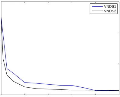
As the step of our final method, we choose to apply VNDS1 to non-demanding problems and VNDS2 to demanding problems. Since this selection method re-quires solving each instance by the CPLEX MIP solver first, it can be very time consuming. Therefore, it would be better to apply another method, based solely on the characteristics of the instances. However, the complexity of such a method would be beyond the scope of this paper, so we decided to present the results obtained with the criterion described above. In Fig. 6 we give the average performance of the two variants VNDS1 and VNDS2 over the prob-lems in the test bed (large-spread instances are not included in this plot2). As predicted, it is clear that in the early stage of the solution process, heuristic VNDS2 improves faster. However, due to the longer time allowed for solving subproblems, VNDS1 improves its average performance later. This pattern of behaviour is even more evident in Fig. 7, where we presented the average gap change over time for demanding problems. However, from Fig. 8, it is clear that a local search in VNDS1 is more effective within a given time limit for non-demanding problems. Even more, Fig. 8 suggests that the time limit for non-demanding problems can be reduced.
(Figures 6-8 come here.)
In Tab. 2, for each of the two variants VNDS1 and VNDS2 we present the time needed until the finally best found solution is reached. The better of the two values for each problem is bolded. As expected, the average time
perfor-2Problemsmarshare1andmarkshare2are specially designed hard small 0-1 instances, with a non-typical behaviour. Being large-spread instances, their behaviour significantly affects the form of the plot 6. The time allowed for instanceNSR8Kis 15 hours, as opposed to 5 hours allowed for all other instances. Furthermore, it takes a very long time (more than 13,000 seconds) to obtain the first feasible solution for this instance. For these reasons, we decided to exclude these three large-spread instances from Fig. 6.
mance of VNDS2 is better, due to the less extensive local search. (Table 2 comes here.)
In Tab. 3 we present VNDS1 and VNDS2 objective values and CPLEX run-ning time for reaching the final solution for all instances in the test bed. The results for demanding problems, i.e., rows where CPLEX time is greater than 12,000 seconds (36,000 seconds for NSR8K instance), are typewritten in italic font, and the better of the two objective values is further bolded. The value selected according to our automatic rule is marked with an asterisk.
(Table 3 comes here.)
From the results shown in Tab. 3, we can see that by applying our automatic rule for selecting one of the two parameters settings, we choose the better of the two variants in 24 out of 29 cases (i.e., in 83% of cases). This further justi-fies our classification of problems and the automatic rule for selection between VNDS1 and VNDS2. With respect to running time, we chose the better of the two variants in 15 out of 29 cases.
Comparison. In Tab. 4 we present the objective function values for the meth-ods tested. Here we report the values obtained with one of the two parameters settings selected according to our automatic rule (see above explanation). For each instance, the best of the five values obtained in our experiments is bolded, and the values which are better than the currently best known are marked with an asterisk.
(Table 4 comes here.)
It is worth mentioning here that most of the best known published results originate from the paper introducing the RINS heuristic [7]. However, these values were not obtained by pure RINS algorithm, but with hybrids which combine RINS with other heuristics (such as local branching, genetic algorithm, guided dives, etc.). In this paper, however, we evaluate the performance of the pure RINS algorithm, rather than different RINS hybrids. It appears that:
(i) With our VNDS based heuristic we obtained better objective values than the best published so far, for as many as eight test instances out of 29 (markshare1,markshare2,van,biella1,UMTS,nsrand ipx,a1c1s1and sp97ar). VNSB improved the best known result in three cases (markshare1, glass4 and sp97ic), and local branching and RINS obtained it for one instance (NSR8Kanda1c1s1, respectively); CPLEX alone did not improve any of the best known objective values.
(ii) With our VNDS based heuristic we were able to reach the best result among all the five methods in 16 out of 29 cases, whereas the RINS heuristic
obtained the best result in 12 cases, VNS branching in 10 cases, CPLEX alone in 6 and local branching in 2 cases.
In Tab. 5, the values of relative gap in % are provided. The gap is computed as
f−fbest |fbest|
×100,
wherefbest is the better value of the following two: the best known published value, and the best among the five results we have obtained in our experiments. The table shows that our algorithm outperforms on average all other methods; it has a percentage gap of only 0.654%, whereas the default CPLEX has a gap of 32.052%, pure RINS of 20.173%, local branching of 14.807%, and VNS branch-ing of 3.120%.
(Table 5 comes here.)
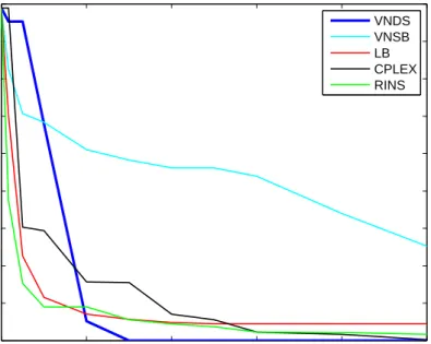
In Fig. 9 we show how the relative gap changes with time for instance biella1. We selected biella1 since it is a small spread instance, where the final gap values of different methods are very similar.
(Figure 9 comes here.)
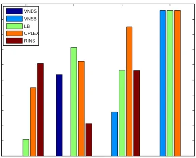
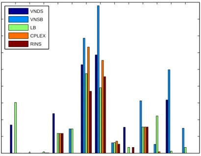
In Fig. 10-13 we graphically display the gaps for all the methods tested. Fig-ures 10-13 show that the large relative gap values in most cases occur because the objective function value achieved by the VNDS algorithm is smaller than that of the other methods.
(Figures 10-13 come here.)
Finally, for all the methods we display the computational time spent until the solution process is finished (see Tab. 6). In computing the average time performance, instanceNSR8Kwas not taken into account, since the time allowed for solving this model was 15 hours, as opposed to 5 hours for all other models. The results show that LB has the best time performance, with an average run-ning time of nearly 6,000 seconds. VNDS is the second best method regarding the computational time, with an average running time of approximately 7,000 seconds. As regards the other methods, VNSB takes more than 8,000 seconds on average, whereas both CPLEX and RINS take more than 11,000 seconds.
(Table 6 comes here.)
The values in Tab. 6 are averages obtained in 10 runs. All the actual values for a particular instance are within the ±5% of the value presented for that instance. Due to the consistency of the CPLEX solver, the objective value (if there is one) obtained starting from a given solution and within a given time limit is always the same. Therefore, the values in Tab. 4-5 are exact (standard deviation over the 10 runs is 0).
Statistical analysis. It is well known that average values are susceptible to outliers, i.e., it is possible that exceptional performance (either very good or very bad) in a few instances influences the overall performance of the algorithm observed. Therefore, comparison between the algorithms based only on the averages (either of the objective function values or of the running times) does not necessarily have to be valid. This is why we have carried out statistical tests to confirm the significance of differences between the performances of the algorithms. Since we cannot make any assumptions about the distribution of the experimental results, we apply a non-parametric (distribution-free) Friedman test [21], followed by the Bonferroni-Dunn [22] post hoc test, as suggested in [23].
Given ` algorithms and N data sets, the Friedman test ranks the perfor-mances of algorithms for each data set (in case of equal performance, average ranks are assigned) and tests if the measured average ranksRj =N1
PN i=1r j i (r j i as the rank of thejth algorithm on theith data set) are significantly different from the mean rank. The statistic used is
χ2 F = 12N `(`+ 1) X` j=1 R2 j− `(`+ 1)2 4 ,
which follows aχ2distribution with`−1 degrees of freedom. Since this statistic proved to be conservative [24], a more powerful version of the Friedman test was developed [24], with the following statistic:
FF = (N−1)χ 2 F N(`−1)−χ2 F ,
which is distributed according to the Fischer’s F-distribution with `−1 and (`−1)(N−1) degrees of freedom. For more details, see [23].
In order to perform the Friedman test, we first rank all the algorithms ac-cording to the objective function values (see Tab. 7) and running times (see Tab. 8). Average ranks by themselves provide a fair comparison of the algo-rithms. Regarding the solution quality, the average ranks of the algorithms over the 29 data sets are 2.43 for VNDS, 2.67 for RINS, 3.02 for VNSB, 3.43 for LB and 3.45 for CPLEX (Tab. 7). Regarding the running times, the average ranks are 2.28 for LB, 2.74 for VNDS, 2.78 for VNSB, 3.52 for RINS, and 3.69 for CPLEX (Tab. 8). These results confirm the conclusions which we draw from observing the average values: that VNDS is the best choice among the five methods regarding the solution quality and the second best choice, after LB, regarding the computational time. However, according to the average rank-ings, the second best method regarding the solution quality is RINS, followed by VNSB, LB and CPLEX, in turn. Regarding the computational time, the ordering of the methods by average ranks is the same as by average values.
(Tables 7-8 come here.)
In order to statistically analyse the difference between the ranks computed, we calculate the value of the FF statistic for ` = 5 algorithms and N = 29
data sets. This value is 2.49 for the objective value rankings and 4.50 for the computational time rankings. Both values are greater than the critical value 2.45 of theF-distribution with (`−1,(`−1)(N−1)) = (4,112) degrees of freedom at the probability level 0.05. Therefore, the null hypothesis that ranks do not significantly differ is rejected. Thus, we conclude that there is a significant difference between the performances of the algorithms, both regarding solution quality and computational time.
Since the equivalence of the algorithms is rejected, we proceed with the post hoc test. The most common post hoc tests used after the Friedman test are the Nemenyi test [25], for pairwise comparisons of all the algorithms, or the Bonferroni-Dunn test [22] when one algorithm of interest (the control algo-rithm) is compared with all the other algorithms (see [23]). In the special case of comparing the control algorithm with all the others, the Bonferroni-Dunn test is more powerful than the Nemenyi test (see [23]), so we decided to use Bonferroni-Dunn test as the post-hoc test with VNDS as the control algorithm. According to the Bonferroni-Dunn test, the performance of two algorithms is significantly different if the corresponding average ranks differ by at least the critical difference
CD=qα
r
`(`+ 1) 6N ,
where qα is the critical value at the probability level α that can be obtained from the corresponding statistical table. For ` = 5, we get q0.05 = 2.498 and
q0.10 = 2.241 (see [23]), so CD = 1.037 for α = 0.05 and CD = 0.931 for
α = 0.10. Regarding the solution quality, from Tab. 9 we can see that, at the probability level 0.10, VNDS is significantly better than LB and CPLEX, since the corresponding average ranks differ by more than CD = 0.931. At the probability level 0.05, post hoc test is not powerful enough to detect any differences. Regarding the computational time, from Tab. 10, we can see that, at the probability level 0.10, VNDS is significantly better than CPLEX, since the corresponding average ranks differ by more thanCD= 0.931. Again, at the probability level 0.05, the post hoc test could not detect any differences. For the graphical display of average rank values in relation to the Bonferroni-Dunn critical difference from the average rank of VNDS as the control algorithm, see Fig. 14-15.
(Tables 9-10 come here.) (Figures 14-15 come here.)
6. Conclusion
In this paper we propose a new approach for solving binary mixed inte-ger programming (MIP) problems. Our method combines hard and soft vari-able fixing: hard fixing is based on the varivari-able neighborhood decomposition search (VNDS) framework, whereas soft fixing introduces pseudo-cuts as in lo-cal branching [6] according to the rules of the variable neighbourhood descent (VND) scheme [8]. In this way we obtain a two-level VNS scheme known as a VNDS heuristic. Moreover, we found a new way to classify instances within a
given test bed. We say that a particular instance is either computationally de-manding or non-dede-manding, depending on the CPU time needed for the default CPLEX optimiser to solve it. Our selection of the particular set of parameters is based on this classification. The VNDS proposed proves to perform well when compared with the state-of-the-art 0-1 MIP solution methods. More precisely, for our solution quality measures we consider several criteria: average percent-age gap, averpercent-age rank according to objective values and the number of times that the method managed to improve the best known published objective. Our experiments show that VNDS proves to be the best in all the aspects stated. In addition, VNDS appears to be the second best method (after LB) regarding the computational time, according to both average computational time and average time performance rank. By performing a Friedman test on our experimental results, we have proven that a significant difference does indeed exist between the algorithms.
Finally, we conclude this work with a few remarks about possible future work. First, our current incumbent updates are based only on the upper bound estimates. Therefore one would expect to speed up the search process by incor-porating the lower bound updates in addition. This can be done for example by introducing new constraints when generating subproblems [11]. Second, as our method is presented as a stand-alone heuristic, i.e., is performed only at the root node of the CPLEX branch-and-bound tree, integrating this method with the branch-and-bound search (allowing it to be performed at each node of the tree) might lead to an even more successful strategy. It is also possible, finally, that this approach may be extended for solving general MIP problems.
Acknowledgements
The present research work has been supported by the International Campus on Safety and Intermodality in Transportation the Nord-Pas-de-Calais Region, the European Community, the Regional Delegation for Research and Technol-ogy, the Ministry of Higher Education and Research, and the National Center for Scientific Research. The authors gratefully acknowledge the support of these institutions. We also would like to thank the referees for their valuable sugges-tions for improving this paper.
References
[1] L. Wolsey, G. Nemhauser, Integer and Combinatorial Optimization (1999). [2] M. Garey, D. Johnson, et al., Computers and Intractability: A Guide to
the Theory of NP-completeness, WH Freeman San Francisco, 1979. [3] A. Soyster, B. Lev, W. Slivka, Zero-One Programming with Many
Vari-ables and Few Constraints, European Journal of Operational Research 2 (3) (1978) 195–201.
[4] P. Shaw, Using Constraint Programming and Local Search Methods to Solve Vehicle Routing Problems, Lecture Notes in Computer Science (1998) 417–431.
[5] R. Ahuja, ¨O. Ergun, J. Orlin, A. Punnen, A survey of very large-scale neighborhood search techniques, Discrete Applied Mathematics 123 (1-3) (2002) 75–102.
[6] M. Fischetti, A. Lodi, Local branching, Mathematical Programming 98 (2) (2003) 23–47.
[7] E. Danna, E. Rothberg, C. L. Pape, Exploring relaxation induced neigh-borhoods to improve mip solutions, Mathematical Programming 102 (1) (2005) 71–90.
[8] P. Hansen, N. Mladenovi´c, D. Uroˇsevi´c, Variable neighborhood search and local branching, Computers and Operations Research 33 (10) (2006) 3034– 3045.
[9] C. Wilbaut, Heuristiques hybrides pour la r´esolution de probl`emes en vari-ables 0-1 mixtes, Ph.D. thesis, Universit´e de Valenciennes, Valenciennes, France (2006).
[10] C. Wilbaut, S. Hanafi, A. Freville, S. Balev, Tabu search: global intensi-fication using dynamic programming, CONTROL AND CYBERNETICS 35 (3) (2006) 579.
[11] C. Wilbaut, S. Hanafi, New convergent heuristics for 0–1 mixed integer programming, European Journal of Operational Research 195 (1) (2009) 62–74.
[12] S. Mitrovi´c-Mini´c, A. Punnen, Very large-scale variable neighborhood search for the generalized assignment problem, accepted for publication in Journal of Interdisciplinary Mathematics.
[13] S. Salhi, A. Al-Khedhairi, Integrating heuristic information into exact methods: The case of the vertex p-centre problem, Accepted for publi-cation in JORS.
[14] R. Bixby, M. Fenelon, Z. Gu, E. Rothberg, R. Wunderling, MIP: Theory and practice – closing the gap (2000) 19–49.
[15] P. Hansen, N. Mladenovi´c, Variable neighborhood search: Principles and applications, European Journal of Operational Research 130 (3) (2001) 449–467.
[16] N. Mladenovi´c, P. Hansen, Variable neighborhood search, Computers and Operations Research 24 (11) (1997) 1097–1100.
[17] P. Hansen, N. Mladenovi´c, Developments of VNS, In: Ribeiro, C. and Hansen, P. (Eds.), Essays and Surveys in Metaheuristics. 415–440.
[18] F. Glover, Heuristics for Integer Programming Using Surrogate Constraints, Decision Sciences 8 (1) (1977) 156–166.
[19] F. Glover, Adaptive memory projection methods for integer programming, In: Rego, C., Alidaee, B. (Eds.), Metaheuristic Optimization Via Memory and Evolution. (2005) 425 – 440.
[20] P. Hansen, N. Mladenovi´c, D. Perez-Britos, Variable Neighborhood Decom-position Search, Journal of Heuristics 7 (4) (2001) 335–350.
[21] M. Friedman, A comparison of alternative tests of significance for the prob-lem of m rankings, The Annals of Mathematical Statistics 11 (1) (1940) 86–92.
[22] O. Dunn, Multiple comparisons among means, Journal of the American Statistical Association (1961) 52–64.
[23] J. Demˇsar, Statistical comparisons of classifiers over multiple data sets, The Journal of Machine Learning Research 7 (2006) 1–30.
[24] R. L. Iman, J. M. Davenport, Approximations of the critical region of the Friedman statistic, Communications in Statistics – Theory and Methods 9 (1980) 571–595.
[25] P. Nemenyi, Distribution-free multiple comparisons, Ph.D. thesis, Prince-ton. (1963).
0 1 2 3 4 5 0 5 10 15 Time (h) Relative gap (%) VNDS1 VNDS2
Figure 6: Relative gap average over all instances in test bed vs. computational time.
0 1 2 3 4 5 0 5 10 15 Time (h) Relative gap (%) VNDS1 VNDS2
0 1 2 3 4 5 0 5 10 15 Time (h) Relative gap (%) VNDS1 VNDS2
Figure 8: Relative gap average over non-demanding instances vs. computational time.
0 1 2 3 4 5 0 1 2 3 4 5 6 7 8 9 biella1 Time (h) Relative gap (%) VNDS VNSB LB CPLEX RINS
markshare1 markshare2 NSR8K 0 100 200 300 400 500 600 700 800 Problems Relative gap (%) VNDS VNSB LB CPLEX RINS
Figure 10: Relative gap values (in %) for large-spread instances.
swath glass4 van net12
0 2 4 6 8 10 12 14 16 18 20 Problems Relative gap (%) VNDS VNSB LB CPLEX RINS
rail507 rail4284c biella1 b1c1s1 b2c1s1 sp97ar sp97ic sp98ar sp98ic 0 0.5 1 1.5 2 2.5 3 Problems Relative gap (%) VNDS VNSB LB CPLEX RINS
Figure 12: Relative gap values (in %) for small-spread instances.
1 2 3 4 5 6 7 8 9 10 11 12 13 0 0.2 0.4 0.6 0.8 1 1.2 1.4 1.6 1.8 Problems Relative gap (%) VNDS VNSB LB CPLEX RINS 1 mkc 2 danoint 3 arki001 4 seymour 5 rail2536c 6 rail2586c 7 rail4872c 8 UMTS 9 roll3000 10 nsrand_ipx 11 a1c1s1 12 a2c1s1 13 tr12−30
VNDS(2.43) VNSB(3.02) LB(3.43) CPLEX(3.45) RINS(2.67) 2
2.5 3 3.5
Algorithms (control algorithm VNDS).
Objective value average ranks.
CD = 0.931 at 0.10 level CD = 1.037 at 0.05 level
Figure 14: Average solution quality performance ranks with respect to Bonferroni-Dunn crit-ical difference from the rank of VNDS as the control algorithm.
VNDS(2.74) VNSB(2.78) LB(2.28) CPLEX(3.69) RINS(3.52) 2
2.5 3 3.5
Algorithms (control algorithm VNDS).
Running time average ranks.
CD = 0.931 at 0.10 level CD = 1.037 at 0.05 level
Figure 15: Average computational time performance ranks with respect to Bonferroni-Dunn critical difference from the rank of VNDS as the control algorithm.
Instance Number of Total number Number of Best published constraints of variables binary variables objective value
mkc 3411 5325 5323 -563.85 swath 884 6805 6724 467.41 danoint 664 521 56 65.67 markshare1 6 62 50 7.00 markshare2 7 74 60 14.00 arki001 1048 1388 415 7580813.05 seymour 4944 1372 1372 423.00 NSR8K 6284 38356 32040 20780430.00 rail507 509 63019 63009 174.00 rail2536c 2539 15293 15284 690.00 rail2586c 2589 13226 13215 947.00 rail4284c 4287 21714 21705 1071.00 rail4872c 4875 24656 24645 1534.00 glass4 396 322 302 1400013666.50 van 27331 12481 192 4.84 biella1 14021 7328 6110 3065084.57 UMTS 4465 2947 2802 30122200.00 net12 14115 14115 1603 214.00 roll3000 2295 1166 246 12890.00 nsrand ipx 735 6621 6620 51360.00 a1c1s1 3312 3648 192 11551.19 a2c1s1 3312 3648 192 10889.14 b1c1s1 3904 3872 288 24544.25 b2c1s1 3904 3872 288 25740.15 tr12-30 750 1080 360 130596.00 sp97ar 1761 14101 14101 662671913.92 sp97ic 1033 12497 12497 429562635.68 sp98ar 1435 15085 15085 529814784.70 sp98ic 825 10894 10894 449144758.40
Instance VNDS1 time (s) VNDS2 time (s) mkc 6303 9003 swath 901 3177 danoint 2362 3360 markshare1 12592 371 markshare2 13572 15448 arki001 4595 4685 seymour 7149 9151 NSR8K 54002 53652 rail507 2150 1524 rail2536c 13284 6433 rail2586c 7897 12822 rail4284c 13066 17875 rail4872c 10939 8349 glass4 3198 625 van 14706 11535 biella1 18000 4452 UMTS 11412 6837 net12 3971 130 roll3000 935 2585 nsrand ipx 14827 10595 a1c1s1 1985 1438 a2c1s1 8403 2357 b1c1s1 4595 5347 b2c1s1 905 133 tr12-30 7617 1581 sp97ar 16933 18364 sp97ic 2014 3085 sp98ar 7173 4368 sp98ic 2724 676 average: 7650 5939
Instance VNDS1 objective value VNDS2 objective value CPLEX time (s) mkc -563.85 -561.94∗ 18000.47 swath 467.41∗ 480.12 1283.23 danoint 65.67 65.67∗ 18000.63 markshare1 3.00∗ 3.00 10018.84 markshare2 8.00∗ 10.00 3108.12 arki001 7580813.05∗ 7580814.51 338.56 seymour 424.00 425.00∗ 18000.59 NSR8K 20758020.00 20752809.00∗ 54001.45 rail507 174.00∗ 174.00 662.26 rail2536c 689.00∗ 689.00 190.194 rail2586c 966.00 957.00∗ 18048.787 rail4284c 1079.00 1075.00∗ 18188.925 rail4872c 1556.00 1552.00∗ 18000.623 glass4 1550009237.59∗ 1587513455.18 3732.31 van 4.82 4.57∗ 18001.10 biella1 3135810.98 3065005.78∗ 18000.71 UMTS 30125601.00 30090469.00∗ 18000.75 net12 214.00 214.00∗ 18000.75 roll3000 12896.00 12930.00∗ 18000.86 nsrand ipx 51360.00 51200.00∗ 13009.09 a1c1s1 11559.36 11503.44∗ 18007.55 a2c1s1 10925.97 10958.42∗ 18006.50 b1c1s1 25034.62 24646.77∗ 18000.54 b2c1s1 25997.84 25997.84∗ 18003.44 tr12-30 130596.00∗ 130596.00 7309.60 sp97ar 662156718.08∗ 665917871.36 11841.78 sp97ic 431596203.84∗ 429129747.04 1244.91 sp98ar 530232565.12∗ 531080972.48 1419.13 sp98ic 449144758.40∗ 451020452.48 1278.13
Table 3: VNDS objective values for two different parameters settings. The CPLEX running time for each instance is also given to indicate the selection of the appropriate setting.
Instance VNDS VNSB LB CPLEX RINS mkc -561.94 -563.85 -560.43 -563.85 -563.85 swath 467.41 467.41 477.57 509.56 524.19 danoint 65.67 65.67 65.67 65.67 65.67 markshare1 3.00∗ 3.00∗ 12.00 5.00 7.00 markshare2 8.00∗ 12.00 14.00 15.00 17.00 arki001 7580813.05 7580889.44 7581918.36 7581076.31 7581007.53 seymour 425.00 423.00 424.00 424.00 424.00 NSR8K 20752809.00 21157723.00 20449043.00∗ 164818990.35 83340960.04 rail507 174.00 174.00 176.00 174.00 174.00 rail2536c 689.00 691.00 691.00 689.00 689.00 rail2586c 957.00 960.00 956.00 959.00 954.00 rail4284c 1075.00 1085.00 1075.00 1075.00 1074.00 rail4872c 1552.00 1561.00 1546.00 1551.00 1548.00 glass4 1550009237.59 1400013000.00∗ 1600013800.00 1575013900.00 1460007793.59 van 4.57∗ 4.84 5.09 5.35 5.09 biella1 3065005.78∗ 3142409.08 3078768.45 3065729.05 3071693.28 UMTS 30090469.00∗ 30127927.00 30128739.00 30133691.00 30122984.02 net12 214.00 255.00 255.00 255.00 214.00 roll3000 12930.00 12890.00 12899.00 12890.00 12899.00 nsrand ipx 51200.00∗ 51520.00 51360.00 51360.00 51360.00 a1c1s1 11503.44∗ 11515.60 11554.66 11505.44 11503.44∗ a2c1s1 10958.42 10997.58 10891.75 10889.14 10889.14 b1c1s1 24646.77 25044.92 24762.71 24903.52 24544.25 b2c1s1 25997.84 25891.66 25857.17 25869.40 25740.15 tr12-30 130596.00 130985.00 130688.00 130596.00 130596.00 sp97ar 662156718.08∗ 662221963.52 662824570.56 670484585.92 662892981.12 sp97ic 431596203.84 427684487.68∗ 428035176.96 437946706.56 430623976.96 sp98ar 530232565.12 529938532.16 530056232.32 536738808.48 530806545.28 sp98ic 449144758.40 449144758.40 449226843.52 454532032.48 449468491.84
Instance VNDS VNSB LB CPLEX RINS mkc 0.337 0.001 0.607 0.001 0.001 swath 0.000 0.000 2.174 9.017 12.149 danoint 0.000 0.000 0.005 0.000 0.000 markshare1 0.000 0.000 300.000 66.667 133.333 markshare2 0.000 50.000 75.000 87.500 112.500 arki001 0.000 0.001 0.015 0.003 0.003 seymour 0.473 0.000 0.236 0.236 0.236 NSR8K 1.485 3.466 0.000 705.999 307.554 rail507 0.000 0.000 1.149 0.000 0.000 rail2536c 0.000 0.290 0.290 0.000 0.000 rail2586c 1.056 1.373 0.950 1.267 0.739 rail4284c 0.373 1.307 0.373 0.373 0.280 rail4872c 1.173 1.760 0.782 1.108 0.913 glass4 10.714 0.000 14.286 12.500 4.285 van 0.000 5.790 11.285 17.041 11.251 biella1 0.000 2.525 0.449 0.024 0.218 UMTS 0.000 0.124 0.127 0.144 0.108 net12 0.000 19.159 19.159 19.159 0.000 roll3000 0.310 0.000 0.070 0.000 0.070 nsrand ipx 0.000 0.625 0.313 0.313 0.313 a1c1s1 0.000 0.106 0.445 0.017 0.000 a2c1s1 0.636 0.996 0.024 0.000 0.000 b1c1s1 0.418 2.040 0.890 1.464 0.000 b2c1s1 1.001 0.589 0.455 0.502 0.000 tr12-30 0.000 0.298 0.070 0.000 0.000 sp97ar 0.000 0.010 0.101 1.258 0.111 sp97ic 0.915 0.000 0.082 2.399 0.687 sp98ar 0.079 0.023 0.046 1.307 0.187 sp98ic 0.000 0.000 0.018 1.199 0.072 average gap: 0.654 3.120 14.807 32.052 20.173
Instance VNDS VNSB LB CPLEX RINS mkc 9003 11440 585 18000 18000 swath 901 25 249 1283 558 danoint 3360 112 23 18001 18001 markshare1 12592 8989 463 10019 18001 markshare2 13572 14600 7178 3108 7294 arki001 4595 6142 10678 339 27 seymour 9151 15995 260 18001 18001 NSR8K 53651 53610 37664 54001 54002 rail507 2150 17015 463 662 525 rail2536c 13284 6543 3817 190 192 rail2586c 12822 15716 923 18049 18001 rail4284c 17875 7406 16729 18189 18001 rail4872c 8349 4108 10431 18001 18001 glass4 3198 10296 1535 3732 4258 van 11535 5244 15349. 18001 18959 biella1 4452 18057 9029 18001 18001 UMTS 6837 2332 10973 18001 18001 net12 130 3305 3359 18001 18001 roll3000 2585 594 10176 180001 14193 nsrand ipx 10595 6677 16856 13009 11286 a1c1s1 1438 6263 15340 18008 18001 a2c1s1 2357 690 2102 18007 18002 b1c1s1 5347 9722 9016 18000 18001 b2c1s1 133 16757 1807 18003 18001 tr12-30 7617 18209 2918 7310 4341 sp97ar 16933 5614 7067 11842 8498 sp97ic 2014 7844 2478 1245 735 sp98ar 7173 6337 1647 1419 1052 sp98ic 2724 4993 2231 1278 1031 average time 6883 8103 5846 11632 11606 Table 6: Running times (in seconds) for all the 5 methods tested.
Instance VNDS VNSB LB CPLEX RINS mkc 4.00 2.00 5.00 2.00 2.00 swath 1.50 1.50 3.00 4.00 5.00 danoint 2.50 2.50 5.00 2.50 2.50 markshare1 1.50 1.50 5.00 3.00 4.00 markshare2 1.00 2.00 3.00 4.00 5.00 arki001 1.00 2.00 5.00 4.00 3.00 seymour 5.00 1.00 3.00 3.00 3.00 NSR8K 2.00 3.00 1.00 5.00 4.00 rail507 2.50 2.50 5.00 2.50 2.50 rail2536c 2.00 4.50 4.50 2.00 2.00 rail2586c 3.00 5.00 2.00 4.00 1.00 rail4284c 3.00 5.00 3.00 3.00 1.00 rail4872c 4.00 5.00 1.00 3.00 2.00 glass4 3.00 1.00 5.00 4.00 2.00 van 1.00 2.00 3.50 5.00 3.50 biella1 1.00 5.00 4.00 2.00 3.00 UMTS 1.00 3.00 4.00 5.00 2.00 net12 1.50 4.00 4.00 4.00 1.50 roll3000 5.00 1.50 3.50 1.50 3.50 nsrand ipx 1.00 5.00 3.00 3.00 3.00 a1c1s1 1.50 4.00 5.00 3.00 1.50 a2c1s1 4.00 5.00 3.00 1.50 1.50 b1c1s1 2.00 5.00 3.00 4.00 1.00 b2c1s1 5.00 4.00 2.00 3.00 1.00 tr12-30 2.00 5.00 4.00 2.00 2.00 sp97ar 1.00 2.00 3.00 5.00 4.00 sp97ic 4.00 1.00 2.00 5.00 3.00 sp98ar 3.00 1.00 2.00 5.00 4.00 sp98ic 1.50 1.50 3.00 5.00 4.00 average ranks 2.43 3.02 3.43 3.45 2.67
Instance VNDS VNSB LB CPLEX RINS mkc 2.00 3.00 1.00 4.50 4.50 swath 4.00 1.00 2.00 5.00 3.00 danoint 3.00 2.00 1.00 4.50 4.50 markshare1 4.00 2.00 1.00 3.00 5.00 markshare2 4.00 5.00 2.00 1.00 3.00 arki001 3.00 4.00 5.00 2.00 1.00 seymour 2.00 3.00 1.00 4.50 4.50 NSR8K 2.50 2.50 1.00 4.50 4.50 rail507 4.00 5.00 1.00 3.00 2.00 rail2536c 5.00 4.00 3.00 1.50 1.50 rail2586c 3.00 2.00 1.00 4.50 4.50 rail4284c 3.00 1.00 2.00 4.00 5.00 rail4872c 2.00 1.00 3.00 4.50 4.50 glass4 2.00 5.00 1.00 3.00 4.00 van 2.00 1.00 3.00 4.00 5.00 biella1 1.00 5.00 2.00 3.50 3.50 UMTS 2.00 1.00 3.00 4.50 4.50 net12 1.00 2.00 3.00 4.50 4.50 roll3000 2.00 1.00 3.00 5.00 4.00 nsrand ipx 2.00 1.00 5.00 4.00 3.00 a1c1s1 1.00 2.00 3.00 4.50 4.50 a2c1s1 3.00 1.00 2.00 4.50 4.50 b1c1s1 1.00 3.00 2.00 4.50 4.50 b2c1s1 1.00 3.00 2.00 4.50 4.50 tr12-30 3.00 5.00 1.00 4.00 2.00 sp97ar 5.00 1.00 2.00 4.00 3.00 sp97ic 3.00 5.00 4.00 2.00 1.00 sp98ar 5.00 4.00 3.00 2.00 1.00 sp98ic 4.00 5.00 3.00 2.00 1.00 average ranks 2.74 2.78 2.28 3.69 3.52
Table 8: Algorithm rankings by the running time values for all instances.
ALGORITHM (average rank) VNSB (3.02) LB (3.43) CPLEX (3.45) RINS (2.67) Difference from VNDS rank (2.43) 0.59 1.00 1.02 0.24 Table 9: Objective value average rank differences from the average rank of the control
algo-rithm VNDS.
ALGORITHM (average rank) VNSB (2.78) LB (2.28) CPLEX (3.69) RINS (3.52) Difference from VNDS rank (2.74) 0.03 -0.47 0.95 0.78 Table 10: Running time average rank differences from the average rank of the control algorithm