Simulation Model to Study Provider Capacity Release Schedules under
Time-Varying Demand Rate for Acute Appointments, Demand for Follow-Up
Appointments, and Time-Dependent No Show Rate
Vera Tilson Ryan Spurr Fangzheng Yuan Joseph Szmerekovsky
Simon Business School College of Business
University of Rochester North Dakota State University
[email protected] [email protected] {fangzheng.yuan,joseph.szmerekovsky}@ndsu.edu
Abstract
We address the problem of scheduling patient appointments in a family medicine clinic. A significant barrier to a clinic’s sustainability is under-utilization of the medical providers it employs. Practically all patient appointments are scheduled some time in advance (from an hour to months ahead), and under-utilization happens because some patients do not keep their appointments and do not provide sufficient notice for the clinic to reschedule another patient into the freed slot. Using a stylized simulation model we investigate an algorithm for appointment capacity release that increases provider utilization.
1. Introduction
Most visits at a family medicine clinic fall into two categories: acute conditions and follow-up visits. Often a visit for an acute problem requires a follow-up visit. Acute appointments are usually requested over the phone, while follow-up appointments are normally scheduled in the clinic immediately after a visit.
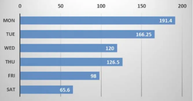
Requests for acute appointments are not uniform throughout the work week, nor are they uniform throughout the day. Figure 1 shows the volume of patient calls to the clinic by day of the week.
The data was collected from a clinic we studied as the motivation for this paper. The data shows only the calls answered by the clinic staff, so demand data is censored. The clinic operates fewer hours on Saturday than on other days of the week, it also does not operate on Sundays. Still the data shows a pattern that is common to many healthcare settings: higher call volume (and, by proxy, demand for acute appointments) on some days than others.
Figure 1: Clinic Call Volume by Day of the Week
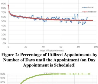
There is another feature of the problem important to note: whether or not a patient utilizes the appointment is related to how far in advance it is scheduled. Referring again to the data from the clinic that motivated our paper, Figure 2 shows the estimated probability that a scheduled appointment is utilized by a patient. The probability decreases with the number of days until the appointment.
In the clinic we examined, as the number of days until appointment reached 80, only half of the appointments were kept. To be clear, the no-show rate was closer to 20% rather than to 50%, because (a) half of all the appointments were scheduled out no more than ten days from the day of the request – as shown in Figure 3,and (b) when appointments were cancelled far enough in advance, it was possible for the time slot to be used for an appointment with another patient.
The clinic’s current practice is to make slots available for scheduling as the day of the appointment nears. So, for example, on any given date, 𝑥𝑥 slots become available for scheduling of appointments six months out, 𝑦𝑦 additional slots become available for scheduling of appointments four weeks out, 𝑧𝑧 additional slots become available for scheduling of appointments one week out, etc. Using a stylized model and a simulation, we examine whether an alternative algorithm for the release of appointment slots can lead Proceedings of the 52nd Hawaii International Conference on System Sciences | 2019
to higher utilization. The capacity release policy we investigate takes into consideration not only the days until the appointment, but also the expected volume of acute requests on that day.
Figure 2: Percentage of Utilized Appointments by Number of Days until the Appointment (on Day
Appointment is Scheduled)
Figure 3: Cumulative Distribution of Scheduled Appointments by Days till Appointment
2.
Literature Review
How long a patient waits to be seen by a medical provider up to the day of the appointment (measured in days), and in the provider’s office on the day of the appointment (measured in minutes) are proxies for patient convenience. Currently several medical appointment scheduling approaches are in use. They represent various tradeoffs between provider utilization and patient convenience [1]. With single booking (also termed fixed and stream scheduling) each patient is given a specific appointment time. The goal of the approach is to keep a steady patient flow with the shortest in-office waiting time for patients. The wave scheduling method attempts to lessen the impact of patient tardiness on the day of the appointment. Multiple patients are assigned the same arrival time and are seen in the order in which they arrive. Clustered scheduling groups patients with similar symptoms or treatment procedures within the same time period of the day or on the same day of the week. This method is often used for physical examinations, diagnostic procedures, and
pregnancy/ gynecology tests. This method reduces variability in service times, reducing in-office waiting time, but possibly increasing the number of days until the appointment.
According to a Merritt Hawkins 2017 survey it takes an average of 24.1 days to schedule a new patient physician appointment in fifteen of the largest cities in the United States, up 30% from 2014 [2]. From the patient’s perspective, long waiting times may cause worse general health perceptions, reduce patient’s life quality, and raise levels of anxiety [3]. It is thought that as a consequence, patients have lower satisfaction and respond with more negative reactions such as cancellations and no shows [4]. It has been shown that waiting times are positively correlated with no show rates [5]. Ryu and Lee [5] noted that longer appointment waits sometimes led to higher costs from the patient’s side (or insurance company) and therefore higher profit for the provider. They hypothesized that this may be one of the reasons waiting times are increasing. Even though long waiting times cause no shows and patient dissatisfaction, reducing waiting time is challenging: Shortening waiting time requires investment in systems. Although some health systems choose to invest in shortening waiting times to improve their competitiveness and efficiency, many choose to lower no shows without addressing long waiting times [5]. With open access booking (also termed advanced access and same-day appointments) patients make an appointment on the day they want to be seen [6]. This methodology has been shown to decrease patients’ wait times and to improve practice efficiency [7-9]. One of the issues in practices where patients need follow-up appointments is what percentage of capacity should be reserved for open-access. Overbooking is a practice of scheduling multiple patients into the same time slot to alleviate the underutilization due to patient no-shows. Although overbooking is a common scheduling paradigm to reduce patients’ no-shows, it increases patient in-office wait times as well as provider overtime [8].
In the operations management literature, outpatient appointment scheduling (OAS) has been examined through a number of lenses relating to measures of the objective, the time horizon, as well as modeling and solution methodologies [10, 11]. For example, Min and Yih used an infinite horizon MDP model to study the problem of managing a waiting list for elective surgery [12]. Gocgun and Puterman [13] formulated as an MDP the problem of scheduling patients for chemotherapy sessions which required appointments at specific future days within a treatment specific time window. Gupta and Wang [14] used an MDP model to obtain booking policies to decide when to accept or deny appointment requests taking into consideration patients’ preferences.
A newsvendor-type model was used by Green, Savin, and Wang [15] in proposing a profit-maximizing allocation of scheduled and non-scheduled time slots for a diagnostic service. Qu et al. [16] proposed an efficient procedure to select the percentage of capacity to allocate for open appointments in an open access scheduling system under the objective of increasing the average number of patients seen while reducing variability. Nguyen, Sivakumar, and Graves used a deterministic model to optimally allocate capacity among two demand sources: first-time patients and follow-up patients [17].
Our setting is similar to the one studied in [18] , where Qu et al. introduced a single-stage stochastic programming model to determine the optimal percentage of a provider’s daily capacity to allocate for open-access appointments. They investigated the sensitivity of this decision to no-show rates, and to the characteristics of demand distribution. Our model includes additional features: time-varying demand rate, demand for follow-up appointments, and wait-time-dependent cancellations and no-shows. Given the many real-world features of our model, we are unable to study it analytically. Thus, we experiment with a simulation model to derive initial insights about the effect of various parameters on the system’s performance. We also note that the yield and capacity management literature is highly relevant to our study.
3.
Description of the Model
The state of the system at the start of a time period 𝑡𝑡 is described by 𝐻𝐻variables, each variable representing the current state of the schedule 𝑡𝑡+ℎ period into the future, where ℎ ∈[0,𝐻𝐻 −1]. The state of the schedule in the future is described by the variable 𝑠𝑠𝑡𝑡+ℎ , the number of appointment slots that have been scheduled up to time 𝑡𝑡. At the start of the period, a decision is made what capacity will be available in each of the next ℎ periods to schedule the appointments. The decisions is a set {𝑟𝑟𝑡𝑡+ℎ}. Next, four uncertainties are realized: (a) some of the appointments scheduled over the 𝐻𝐻-period horizon are cancelled by patients, (b) the demand for acute appointments is realized and these appointments are scheduled subject to released capacity, (c) patients attend some of the appointments scheduled for period 𝑡𝑡 -- the number of appointment slots that end up being utilized is denoted with 𝑈𝑈𝑡𝑡, (d) some proportion of patients who attended their appointments in period 𝑡𝑡generate demand for follow-up appointments. These appointments are scheduled as well, subject to released capacity. Assuming that total available (released or not) capacity is the same every day, capacity releasing
policies {𝑟𝑟𝑡𝑡+ℎ} can be compared using the average number of attended appointments:
𝑙𝑙𝑙𝑙𝑙𝑙
𝑇𝑇→∞
∑𝑇𝑇𝑡𝑡=0𝐸𝐸[𝑈𝑈𝑡𝑡]
𝑇𝑇 .
The criteria could also include penalties for appointment that are requested but not scheduled due to insufficient capacity.
As discussed in the introduction, while the quantity of daily requests, of cancellations and the need for follow-up appointments is uncertain, there is historical information on these quantities which suggests some features for a mathematical model. For example, follow-up appointments are usually scheduled some time into the future, so that the effects of a treatment might be observed. So we modeled follow-up appointments as appointments that are scheduled no earlier than 𝐻𝐻𝑓𝑓 periods from the day of the request, while acute appointments are scheduled no later than 𝐻𝐻𝑎𝑎 periods from the time of the request. A follow-up appointment arises from an attended appointment, so we assume that the number of requests for follow-up appointments in period 𝑡𝑡 is binomially distributed with parameter 𝑛𝑛equal to the number of appointments that were utilized in period 𝑡𝑡, and parameter 𝑝𝑝𝑓𝑓 as the probability of any one attended appointment requiring a follow-up.
Another feature that we sought to model is that the likelihood of a cancellation or of a no-show increases with the time interval between when a request is made and when the appointment is scheduled. We model this behavior as follows: for each appointment there is a probability 𝛾𝛾 that on any given day a patient will decide not to keep the appointment (if that decision has not been made by the patient previously). When the patient decides not to keep the appointment, there is a probability 𝛽𝛽, that the patient will notify the clinic of that decision -- which will allow the clinic to release the associated capacity.
We also modeled the cyclical nature of the arrival rate of requests for acute appointments. In the numerical experiments which are discussed later we used a parsimonious model alternating periods of high and low demand rates. Another simplification that we used in the model was ignoring that appointments are normally made for a particular time of day -- we assumed that acute appointments requested in period 𝑡𝑡 are scheduled for period 𝑡𝑡 up to the available capacity, then what cannot be accommodated in period 𝑡𝑡 is scheduled for period 𝑡𝑡+ 1, and so on up to 𝑡𝑡+𝐻𝐻𝑎𝑎. Similarly, follow-up appointments requested in period 𝑡𝑡 are scheduled for period 𝑡𝑡+𝐻𝐻𝑓𝑓, what cannot be accommodated there -- for period 𝑡𝑡+𝐻𝐻𝑓𝑓+1, and so on, up until the end of planning horizon. The requests that cannot be accommodated, due to insufficient capacity, are lost.
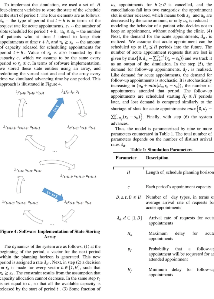
To implement the simulation, we used a set of 𝐻𝐻 four-element variables to store the state of the schedule at the start of period 𝑡𝑡. The four elements are as follows: 𝜆𝜆ℎ -- the type of period that 𝑡𝑡+ℎ is in terms of the
request rate for acute appointments, 𝑠𝑠ℎ -- the number of slots scheduled for period 𝑡𝑡+ℎ, 𝑢𝑢ℎ≤ 𝑠𝑠ℎ -- the number of patients who at time 𝑡𝑡 intend to keep their appointments at time 𝑡𝑡+ℎ, and 𝑟𝑟ℎ≥ 𝑠𝑠ℎ -- the amount of capacity released for scheduling appointments for period 𝑡𝑡+ℎ. Value of 𝑟𝑟ℎ is also bounded by the capacity 𝑐𝑐, which we assume to be the same every period so 𝑟𝑟ℎ≤ 𝑐𝑐. In terms of software implementation, we stored these state entities using an array, and redefining the virtual start and end of the array every time we simulated advancing time by one period. This approach is illustrated in Figure 4.
Figure 4: Software Implementation of State Storing Array
The dynamics of the system are as follows: (1) at the beginning of the period, a vector for the next period within the planning horizon is generated. This new period is assigned a rate 𝜆𝜆𝐻𝐻. Next, in step (2) a decision on 𝑟𝑟ℎ is made for every vector ℎ ∈[1,𝐻𝐻], such that 𝑟𝑟ℎ≥ 𝑠𝑠ℎ. The constraint results from the assumption that
capacity allocation cannot decrease. In the same step 𝑟𝑟0 is set equal to 𝑐𝑐, so that all the available capacity is released by the start of period 𝑡𝑡 . (3) Some fraction of
𝑢𝑢ℎ appointments for ℎ ≥0 is cancelled, and the
cancellations fall into two categories: the appointment slot is either released, which means both 𝑠𝑠ℎ and𝑢𝑢ℎare decreased by the same amount, or only 𝑢𝑢ℎ is reduced -- modeling the behavior of a patient who decides not to keep an appointment, without notifying the clinic. (4) Next, the demand for the acute appointments, 𝑑𝑑𝑎𝑎, is realized. We assume that acute appointment can be scheduled up to 𝐻𝐻𝑎𝑎≤ 𝐻𝐻 periods into the future. The number of acute appointment requests that are lost is given by 𝑙𝑙𝑚𝑚𝑥𝑥�0,𝑑𝑑𝑎𝑎− ∑ℎ=0𝐻𝐻𝑎𝑎−1(𝑟𝑟ℎ− 𝑠𝑠ℎ)� and we track it as an output of the simulation. In the step (5), the demand for follow-up appointments, 𝑑𝑑𝑓𝑓, is realized. Like demand for acute appointments, the demand for follow-up appointments is stochastic. It is stochastically increasing in (𝑢𝑢0+𝑙𝑙𝑙𝑙𝑛𝑛{𝑑𝑑𝑎𝑎,𝑟𝑟0− 𝑠𝑠0}), the number of
appointments attended that period. The follow-up appointments are scheduled starting 𝐻𝐻𝑓𝑓 ≤ 𝐻𝐻 periods later, and lost demand is computed similarly to the shortage of slots for acute appointments: 𝑙𝑙𝑚𝑚𝑥𝑥 �0,𝑑𝑑𝑓𝑓− ∑𝐻𝐻ℎ=𝐻𝐻𝑓𝑓(𝑟𝑟ℎ− 𝑠𝑠ℎ)�. Finally, with step (6) the system
advances.
Thus, the model is parameterized by nine or more parameters enumerated in Table 1. The total number of parameters depends on the number of distinct arrival rates 𝜆𝜆𝑑𝑑.
Table 1: Simulation Parameters Parameter Description
𝐻𝐻 Length of schedule planning horizon
𝑐𝑐 Each period’s appointment capacity 𝐷𝐷,𝑠𝑠.𝑡𝑡.𝐷𝐷 ≤ 𝐻𝐻 Number of day types, in terms of
average arrival rate of requests for acute appointments
𝜆𝜆𝑑𝑑,𝑑𝑑 ∈[1,𝐷𝐷] Arrival rate of requests for acute
appointments
𝐻𝐻𝑎𝑎 Maximum delay for acute
appointments
𝑝𝑝𝑓𝑓 Probability that a follow-up
appointment will be requested for an attended appointment
𝐻𝐻𝑓𝑓 Minimum delay for follow-up
𝛾𝛾 One period probability of a patient deciding not to keep a scheduled appointment
𝛽𝛽 Probability that a patient who decided not to keep the appointment, notifies the clinic of the cancellation
3.1. Computational Experiments
For all the numerical experiments we conducted, we set per-period capacity 𝑐𝑐= 10 , considered two different demand types, so 𝐷𝐷= 2, assumed a planning horizon of four periods, so 𝐻𝐻= 4. We set the maximum delay for acute appointments 𝐻𝐻𝑎𝑎= 2, and minimum delay for follow-up appointments 𝐻𝐻𝑓𝑓 = 2.
For the other inputs we experimented with the following sets of parameters: 𝛾𝛾 ∈{0.1,0.25} , 𝛽𝛽 ∈
{0.3,0.7} , 𝑝𝑝𝑓𝑓∈{0.2,0.5} . These were chosen to
experiment with the high and low probabilities of cancellations, no-shows, and follow-up appointments.
We modeled average daily demand for acute appointments as 𝜆𝜆𝑎𝑎𝑎𝑎𝑎𝑎
=
10-8.5𝑝𝑝𝑓𝑓 - assuming 85% average utilization. Given two types of periods that alternate we modeled average demand in periods with high demand as 𝜆𝜆ℎ𝑖𝑖𝑎𝑎ℎ=𝜃𝜃𝜆𝜆𝑎𝑎𝑎𝑎𝑎𝑎, and in periods with low demand as 𝜆𝜆𝑙𝑙𝑙𝑙𝑙𝑙= (2− 𝜃𝜃)𝜆𝜆𝑎𝑎𝑎𝑎𝑎𝑎, with 𝜃𝜃 ∈{1,1.2,1.5}to understand the effect of demand variability. For the simulation, we modeled demand as arising from a Poisson distribution with the rate 𝜆𝜆.Finally, we examined six different capacity release policies. The policies enumerated in Table 2, are described by the number of slots released at each point in time.
Table 2: Capacity Release Policies Studied Computationally
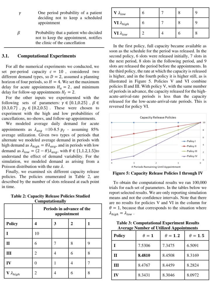
Periods in advance of the appointment Policy 4 3 2 1 I 10 II 6 7 8 9 III 2 4 6 8 IV 0 1 4 7 V𝜆𝜆ℎ𝑖𝑖𝑎𝑎ℎ 2 4 6 8 V𝜆𝜆𝑙𝑙𝑙𝑙𝑙𝑙 6 7 8 9 VI𝜆𝜆ℎ𝑖𝑖𝑎𝑎ℎ 6 7 8 9 VI𝜆𝜆𝑙𝑙𝑙𝑙𝑙𝑙 2 4 6 8
In the first policy, full capacity became available as soon as the schedule for the period was released. In the second policy, 6 slots were released initially, 7 slots in the next period, 8 slots in the following period, and 9 slots are released the period before the appointments. In the third policy, the rate at which the capacity is released is higher, and in the fourth policy it is higher still, as is illustrated in Figure 5. Policies V and VI combine policies II and III. With policy V, with the same number of periods in advance, the capacity released for the high-acute-arrival-rate periods is less than the capacity released for the low-acute-arrival-rate periods. This is reversed for policy VI.
Figure 5: Capacity Release Policies I through IV
To obtain the computational results we ran 100,000 trials for each set of parameters. In the tables below we report selected results. We are only reporting simulation means and not the confidence intervals. Note that there are no results for policies V and VI in the column for 𝜃𝜃= 1, because that corresponds to the situation where 𝜆𝜆ℎ𝑖𝑖𝑎𝑎ℎ=𝜆𝜆𝑙𝑙𝑙𝑙𝑙𝑙 .
Table 3: Computational Experiment Results Average Number of Utilized Appointments Policy 𝜃𝜃=𝟏𝟏 𝜃𝜃=𝟏𝟏.𝟐𝟐 𝜃𝜃=𝟏𝟏.𝟓𝟓
I 7.5306 7.3475 6.5091
II 8.4810 8.4508 8.3169
III 8.4767 8.4459 8.2824
V
N/A
8.4547 8.3228
VI 8.4483 8.2843
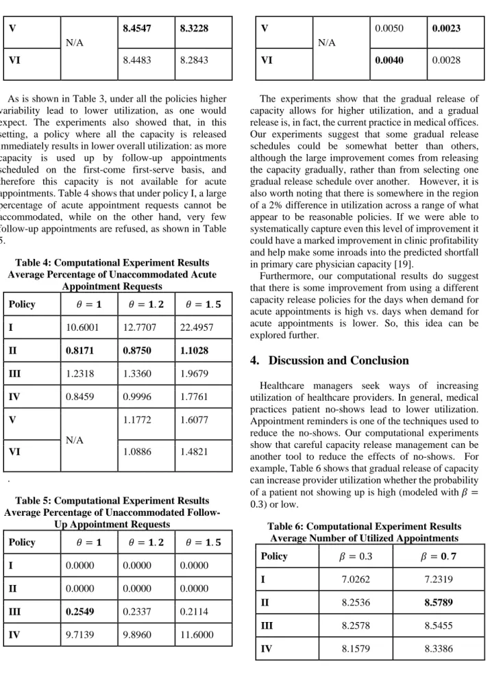
As is shown in Table 3, under all the policies higher variability lead to lower utilization, as one would expect. The experiments also showed that, in this setting, a policy where all the capacity is released immediately results in lower overall utilization: as more capacity is used up by follow-up appointments scheduled on the first-come first-serve basis, and therefore this capacity is not available for acute appointments. Table 4 shows that under policy I, a large percentage of acute appointment requests cannot be accommodated, while on the other hand, very few follow-up appointments are refused, as shown in Table 5.
Table 4: Computational Experiment Results Average Percentage of Unaccommodated Acute
Appointment Requests Policy 𝜃𝜃=𝟏𝟏 𝜃𝜃=𝟏𝟏.𝟐𝟐 𝜃𝜃=𝟏𝟏.𝟓𝟓 I 10.6001 12.7707 22.4957 II 0.8171 0.8750 1.1028 III 1.2318 1.3360 1.9679 IV 0.8459 0.9996 1.7761 V N/A 1.1772 1.6077 VI 1.0886 1.4821 .
Table 5: Computational Experiment Results Average Percentage of Unaccommodated
Follow-Up Appointment Requests Policy 𝜃𝜃=𝟏𝟏 𝜃𝜃=𝟏𝟏.𝟐𝟐 𝜃𝜃=𝟏𝟏.𝟓𝟓 I 0.0000 0.0000 0.0000 II 0.0000 0.0000 0.0000 III 0.2549 0.2337 0.2114 IV 9.7139 9.8960 11.6000 V N/A 0.0050 0.0023 VI 0.0040 0.0028
The experiments show that the gradual release of capacity allows for higher utilization, and a gradual release is, in fact, the current practice in medical offices. Our experiments suggest that some gradual release schedules could be somewhat better than others, although the large improvement comes from releasing the capacity gradually, rather than from selecting one gradual release schedule over another. However, it is also worth noting that there is somewhere in the region of a 2% difference in utilization across a range of what appear to be reasonable policies. If we were able to systematically capture even this level of improvement it could have a marked improvement in clinic profitability and help make some inroads into the predicted shortfall in primary care physician capacity [19].
Furthermore, our computational results do suggest that there is some improvement from using a different capacity release policies for the days when demand for acute appointments is high vs. days when demand for acute appointments is lower. So, this idea can be explored further.
4.
Discussion and Conclusion
Healthcare managers seek ways of increasing utilization of healthcare providers. In general, medical practices patient no-shows lead to lower utilization. Appointment reminders is one of the techniques used to reduce the no-shows. Our computational experiments show that careful capacity release management can be another tool to reduce the effects of no-shows. For example, Table 6 shows that gradual release of capacity can increase provider utilization whether the probability of a patient not showing up is high (modeled with 𝛽𝛽= 0.3) or low.
Table 6: Computational Experiment Results Average Number of Utilized Appointments Policy 𝛽𝛽= 0.3 𝛽𝛽=𝟎𝟎.𝟕𝟕
I 7.0262 7.2319
II 8.2536 8.5789
III 8.2578 8.5455
V 8.2699 8.5662
VI 8.2448 8.5644
Real-world characteristics of demand for medical appointments has a number of features that make non-computational approaches challenging. These features include the demand for follow-up appointments, the probability of no-show or cancellations when an appointment is scheduled further into the future, and time-varying demand rates. Further research is needed to derive structural properties of optimal policies and computational algorithms for effectively dealing with the curse of dimensionality to compute capacity release policies that would increase utilization in healthcare appointment setting.
5.
References
[1] K. Bonewit-West, S.A. Hunt, E. Applegate, Today's Medical Assistant: Clinical and Administrative Procedures, Elsevier Health Sciences2012.
[2] Merritt Hawkins Team, 2017 Survey of Physician Appointment Wait Times and Medicare and Medicaid Acceptance Rates, AMN HEALTHCARE SERVICES INC, Dallas, TX 2017.
[3] J. Oudhoff, D. Timmermans, D. Knol, A. Bijnen, G. Van der Wal, Waiting for elective general surgery: impact on health related quality of life and psychosocial consequences, BMC Public Health, 7 (2007) 164. [4] D. Ansell, J.A. Crispo, B. Simard, L.M. Bjerre, Interventions to reduce wait times for primary care appointments: a systematic review, BMC Health Services Research, 17 (2017) 295.
[5] J. Ryu, T.H. Lee, The waiting game—why providers may fail to reduce wait times, New England Journal of Medicine, 376 (2017) 2309-2311.
[6] N. Liu, S. Ziya, V.G. Kulkarni, Dynamic scheduling of outpatient appointments under patient no-shows and cancellations, Manufacturing & Service Operations Management, 12 (2010) 347-364.
[7] S. Cameron, L. Sadler, B. Lawson, Adoption of open-access scheduling in an academic family practice, Canadian Family Physician, 56 (2010) 906-911.
[8] L.R. LaGanga, S.R. Lawrence, Clinic overbooking to improve patient access and increase provider productivity, Decision Sciences, 38 (2007) 251-276. [9] A. Mehrotra, L. Keehl-Markowitz, J. Ayanian, Implementation of open access scheduling in primary care: A cautionary tale, JOURNAL OF GENERAL INTERNAL MEDICINE, SPRINGER 233 SPRING STREET, NEW YORK, NY 10013 USA, 2007, pp. 198-198.
[10] A. Ahmadi-Javid, Z. Jalali, K.J. Klassen, Outpatient appointment systems in healthcare: A review of optimization studies, European Journal of Operational Research, 258 (2017) 3-34.
[11] D. Gupta, B. Denton, Appointment scheduling in health care: Challenges and opportunities, IIE Transactions, 40 (2008) 800-819.
[12] D. Min, Y. Yih, Managing a patient waiting list with time-dependent priority and adverse events, RAIRO - Operations Research, 48 (2014) 53-74. [13] Y. Gocgun, M.L. Puterman, Dynamic scheduling with due dates and time windows: an application to chemotherapy patient appointment booking, Health Care Management Science, 17 (2014) 60-76.
[14] D. Gupta, L. Wang, Revenue management for a primary-care clinic in the presence of patient choice, Operations Research, 56 (2008) 576-592.
[15] L.V. Green, S. Savin, B. Wang, Managing patient service in a diagnostic medical facility, Operations Research, 54 (2006) 11-25.
[16] X. Qu, R.L. Rardin, J.A.S. Williams, A mean– variance model to optimize the fixed versus open appointment percentages in open access scheduling systems, Decision Support Systems, 53 (2012) 554-564. [17] T.B.T. Nguyen, A.I. Sivakumar, S.C. Graves, A network flow approach for tactical resource planning in outpatient clinics, Health Care Management Science, 18 (2015) 124-136.
[18] X. Qu, R.L. Rardin, J.A.S. Williams, D.R. Willis, Matching daily healthcare provider capacity to demand in advanced access scheduling systems, European Journal of Operational Research,, 183 (2007) 812-826. [19] S. Porter, Significant primary care, overall physician shortage predicted by 2025, American Academy of Family Physicians, 2015.