Evaluating credal classifiers by utility-discounted predictive accuracy

Contents lists available atSciVerse ScienceDirect

International Journal of Approximate Reasoning

j o u r n a l h o m e p a g e :w w w . e l s e v i e r . c o m / l o c a t e / i j a r

Evaluating credal classifiers by utility-discounted predictive accuracy

Marco Zaffalon

∗

, Giorgio Corani, Denis Mauá

IDSIA, Galleria 2, CH-6928 Manno (Lugano), Switzerland

A R T I C L E I N F O A B S T R A C T

Article history:

Available online 28 June 2012

Predictions made by imprecise-probability models are often indeterminate (that is, set-valued). Measuring the quality of an indeterminate prediction by a single number is im-portant to fairly compare different models, but a principled approach to this problem is currently missing. In this paper we derive, from a set of assumptions, a metric to evaluate the predictions of credal classifiers. These are supervised learning models that issue set-valued predictions. The metric turns out to be made of an objective component, and another that is related to the decision-maker’s degree of risk aversion to the variability of predictions. We discuss when the measure can be rendered independent of such a degree, and provide insights as to how the comparison of classifiers based on the new measure changes with the number of predictions to be made. Finally, we make extensive empirical tests of credal, as well as precise, classifiers by using the new metric. This shows the practical usefulness of the metric, while yielding a first insightful and extensive comparison of credal classifiers.

© 2012 Elsevier Inc. All rights reserved.

1. Introduction

When we use an imprecise-probability model to make predictions, we meet one of the most striking differences of impre-cise probability in comparison to preimpre-cise probability: the impreimpre-cise-probability model can issueindeterminatepredictions. That is, among the set of possible options, the model may drop some of them as sub-optimal, while keeping the entire remaining set as its prediction. The prediction is generally indeterminate as such a set is not necessarily a singleton. Inde-terminate predictions are a crucially important feature of imprecise-probability models: they allow credible, and reliable, predictions to be obtained no matter how scarce is the information available to build a model.

Yet, we should have a way tomeasurehow good is an indeterminate prediction. A major reason is that we need to compare imprecise- with precise-probability models: we should have a simple and possibly shared way to say which one is better in a given application. The same consideration applies when we compare two imprecise-probability models. Ideally, we would like to be able to reward each prediction by a single number, be it determinate or indeterminate. Most probably this would speed up progress in the field, as it would enable comparisons to be automatized over a large number of test applications.

In the case of precise-probability models, there are well-consolidated measures to do this. Let us consider the field of

pattern classification[11], which is the focus of this paper (Section2gives a brief introduction to classification problems). In this case, the predictive models are called (precise)classifiers. A classifier predicts one out of a finite setCof so-called

classes. In this case, correct predictions may be rewarded with 1 and incorrect ones with 0, thus giving rise to the measure of performance called thepredictive accuracyof a classifier: i.e., the proportion of correct predictions it makes.

The situation is very different withcredal classifiers, that is, classifiers that issue set-valued predictions. One of the few proposals to evaluate an indeterminate prediction by a single number can be found in [7]: a prediction made of a set

Kofkclasses is rewarded with 1

/

kif it contains the actual class, and with 0 otherwise. This gives rise to the measure calleddiscounted accuracy, which was borrowed from the field of multi-label classification [22]. The problem here is that no justification is given for discounted accuracy, as the work in [7] points out. In [17], classifiers which return indeterminate

∗_{Corresponding author.}

E-mail addresses:[email protected](M. Zaffalon),[email protected](G. Corani),[email protected](D. Mauá). 0888-613X/$ - see front matter © 2012 Elsevier Inc. All rights reserved.

classifications are evaluated through the F-metric, originally designed for information retrieval problems; but also in this case, there is no actual justification for the choice of this measure. Other than these, the past proposals are either explicitly non-numerical, as the rank test in [7], or require a vector of parameters to evaluate the performance, as in [6]. The latter approach is meaningful, but was conceived to compare credal with precise classifiers, and cannot be easily extended to the more general case; moreover, it is a method that needs supervision so that it does not easily lend itself to be run automatically on many test cases.

In our view, the scarcity of principled numerical evaluation methods for credal classifiers is not accidental: in fact, it is not easy to assign a single number to an indeterminate prediction. Consider the following case: there is avacuousclassifier, which every time predicts the set of all classesC, and arandomone, which picks up a class fromCthrough the uniform distribution. IfCis made of two classes (we say that the classification problem is binary), and we use the predictive accuracy, the random classifier has an expected reward equal to 1

/

2. What should be the expected reward of the vacuous classifier? Both classifiers do not know how to predict the class, but only the vacuous classifier declares it. From this, one might argue that the latter should be rewarded with more than 1

/

2. On the other hand, it is clear also that the vacuous classifier cannot predict the class better than the random one, so that one might argue that it should be rewarded with 1

/

2 too.

In the attempt to address these kinds of problems in the most objective way, we found it useful to regard classifiers as bettors. In the betting framework introduced in Section3, we assume we only know how to value determinate predictions, in particular by 0-1 rewards. In Section4, we extend the framework, in a kind of least-committal way, to credal classifiers: we show that, under reasonable assumptions, indeterminate predictions should be valued according to discounted accuracy. Note, however, that discounted accuracy values the vacuous and the random classifiers the same. This kind of (question-able) effect can be traced back to having deliberately avoided introducing subjective considerations in the evaluation. Still, subjective preferences should be accounted for: we introduce in Section5a decision maker in charge of selecting the ‘best’ classifier in the next bet, and show that preferences can enter the picture through his utility, as a function of discounted accuracy. This defines the measure we propose to evaluate credal classifiers:utility-discounted predictive accuracy. More generally speaking, this shows in a very definite sense how the reliability of a classifier is tightly related to the variability of its predictions, and that the aversion to this variability is what makes some people prefer credal classifier to precise ones. In Section6we briefly discuss how utility-discounted accuracy can equivalently, and quite naturally, be derived also in a framework based on money bets. This illustrates the tight relationship of our approach with finance.

In Section7we discuss an important case where the evaluation can still be made in quite an objective way despite the decision-maker’s subjective preferences, and we relate this to the amount of indeterminacy produced by a credal classifier. In Section8we analyze how the picture changes if we focus on evaluating classifiers in the nextm

≥

1 bets. We show that the difference between precise and credal classifiers decreases with growingm, so that the relative benefits of credal classification are less pronounced for largem.

Section9is entirely devoted to the empirical evaluation of credal classifiers based on utility-discounted accuracy. We start by discussing the choice of sensible utility functions for our aim, that is, the fair comparison of credal classifiers. In Section9.1, we focus the comparison on two classifiers representative of the precise and the credal categories:naive Bayes classifier(NBC [9]) andnaive credal classifier(NCC [25,26,6]). We infer and test them both on artificial data and on 55 real data sets from the well-known UCI repository. This shows, as expected, that NCC yields particular advantages over NBC on small learning sets. In more general conditions the situation is somewhat more balanced, although it tends to be in favor of NCC when the decision maker has strong preferences towards reliability of classification. It is also shown clearly that when the NCC is indeterminate, the NBC issues fragile predictions; this confirms past results in the literature.

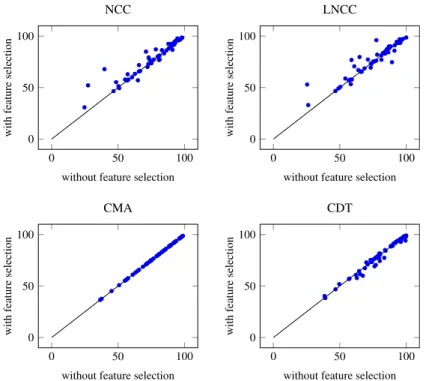
The comparison is extended in Section9.2to other credal classifiers (again on the UCI data sets): a local (that is, lazy) version of NCC [7]; a classifier obtained through imprecise-probabilistic model averaging of NBCs [5]; and a classification tree extended to imprecise probability [1,2]. A thorough analysis highlights different characteristics of the involved credal classifiers, and, at the same time, a substantial balance in their predictive performances (in particular when they are used jointly with feature selection to reduce overfitting). It is worth remarking that this kind of extensive and insightful comparison is made here for the first time, thanks to the availability of utility-discounted accuracy.

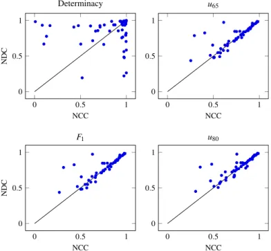
Section9.3is devoted to a detailed comparison of NCC with a set-valued classifier developed within precise probability: thenon-deterministicclassifier (NDC) of Coz et al. [17]. This comparison is interesting because the mentioned classifiers work according to very different principles, even though both yield set-valued classifications. Moreover, the discussion shows how the F-metric used in [17] for comparing classifiers, can be meaningfully re-interpreted as a utility function in our framework. This provided a justification for such a metric that was not available before. The comparison of NCC with NDC gives us the opportunity to consider a related question in Section9.4: the extent to which a fair comparison of classifiers is possible to do when some of them implement the so-calledrejection option: this is a precise-probability tool to issue set-valued classifications that relies on the inspection of the posterior probabilities assigned to the classes.

Our concluding remarks are in Section10.

2. Classification problems

A classification problem is made of objects described byattribute(orfeature) variables, which we group into the sin-gle variableA, and a class variableC. The class variable represents the object’s category. There are finitely many possible

categories, which we identify with their indexes to simplify notation:

{

1

, . . . ,

n

} =:

C. We denote bycthe generic element ofC. The attribute variable represents some characteristics of the object that are related to the class. VariableAtakes values in the setA; we denote byaits generic element. As an example, objects might be patients.Awould represent a patient’s profile: that is, personal information as well as the outcomes of medical tests.Cwould index the patient’s possible diseases. Usually, some values of

(

A

,

C

)

are sampled in an independent and identically distributed way according to a law that is not known a priori. The so-calledlearning setLrecords those values, which are also calledinstancesof

(

A

,

C

)

. The goal of classification is to learn from the learning set a function that maps attributes into classes; we call this function a (precise)

classifier. With reference to the above medical example, the goal would be to understand from data how a patient’s profile is related to disease: a classifier in this case would be a function that takes in input a profile and outputs a prediction about the patient’s disease.

A classifier’s predictions are rewarded through areward matrix

R

. This is ann

×

nmatrix whose generic elementrijis

a number representing the reward obtained by predicting classiwhen the actual class isj. Equivalently, we can regard the reward matrix as a set ofgambles(i.e., bounded random variables)

R

i,i

=

1

, . . . ,

n, each one corresponding to a row of

R

: gamble

R

irepresents the uncertain reward obtained by predicting classiand is defined by

R

i

(

j

)

:=

rij, withj

∈

C. The

reward matrix is an input of the classification problem, in the sense that it is given.

In classification, at least with respect to the machine learning practice, rewards are usually measured in a linear utility scale: although this point is often left implicit, we can deduce it from the observation that the performance of a classifier is usually identified with its expected reward.

A very frequent practice consists also in using just a 0-1 valued reward matrix, which we denote by

I

(Table1shows matrix

I

for the simplest case of a binary classification problem).

Table 1

0–1 Reward matrix for a binary classification problem. Actual class

1 2

Predicted class 1 1 0

2 0 1

In this case, the gamble corresponding to thei-th row of the matrix coincides with the indicator function of set

{

i

}

, which yields

I

i

(

i

)

=

1, and

I

i

(

j

)

=

0 fori

=

j. Accordingly, the performance of a classifier corresponds to the probability of

predicting the actual class. Such a probability is called thepredictive accuracy(or simply theaccuracy) of a classifier. The term ‘accuracy’ is used also for the sample estimate of such a probability. In fact, a classification problem usually comes with a test setT. This set contains a number of sampled instances of

(

A

,

C

)

that are used to evaluate the classifier’s predictive performance by measuring its accuracy on them.

The widespread use of predictive accuracy has probably been favored by its simple interpretation; a more substantial reason could be that the predictive accuracy is particularly convenient to make extensive comparisons of classifiers over many data sets, which is a key component of the machine learning practice. Accordingly, in this paper we focus on the 0-1 valued reward matrix

I

, and as a consequence on measures of accuracy that are not cost sensitive. This is not to say that we support the abuse of 0-1 rewards to evaluate classifiers: we believe that a careful elicitation of rewards would arguably lead in many cases to a reward matrix more general than

I

. There are indeed a number of measures alternative to predictive accuracy proposed in the field of classification for the case where different types of error, such as false positives and false negatives, should be given different rewards. This is the case, for instance, of so-called sensitivity and specificity measures [11]. On the other hand, the case of 0-1 rewards makes the treatment easier and at the same time it is arguably one of the most important cases to consider.

So far we have introduced the traditional view of classification, where the predictions issued by (precise) classifiers are made of single classes. This view has been generalized through the introduction of credal classifiers [25,27]. Acredal classifier

is also a function learned from setL, but it maps the attributes of an instance into a non-empty setK

⊆

Cofk

:= |

K

|

classes in general. We call this a set-valued classification. We also say that the classification isdeterminatewhenk

=

1, andindeterminateotherwise. When a classification is fully indeterminate, that is, whenK

=

C, we call itvacuous. Similarly, thevacuous classifieris the one that always issues vacuous predictions. To each credal classifier it is possible to associate a determinate classifier that outputs predictions by choosing every time a class uniformly at random1 from the output setK

of the credal classifier. We call this theK-random classifier; when the related credal classifier is the vacuous one, we just call it therandom classifier.

Evaluating a credal classifier can be regarded as the problem of defining an ‘extended’ reward matrix, which associates a reward gamble to each non-empty subset of classes. For instance, suppose that one believes that the vacuous and the random classifiers should be evaluated equally in a binary classification problem characterized by matrix

I

. The corresponding extended reward matrix is given in Table2.

1

Table 2

An extended reward matrix for a binary classification problem featuring reward matrixI. This specific extended reward matrix, which values the random and the vacuous classifiers the same, originates the metric called discounted accuracy in [7] (see also Section4). Observe that in problems with more than two classes, there will obviously be more rows to fill with the appropriate rewards gambles.

Actual class 1 2 Predicted class 1 1 0 2 0 1 {1,2} 0.5 0.5

3. Introducing the betting framework

In order to make the comparison of credal classifiers as objective as possible, we introduce the idea of a betting framework. We define the framework for a traditional problem of classification, where classifiers issue determinate predictions. In Section4we will extend the framework to credal classification.

In the framework under consideration, we have two classifiers, which we would like to compare, that have already been inferred from data (so that there is no further learning, only an evaluation stage). We build the framework in such a way that the better the predictions a classifier issues the more it earns. In other words, the idea is that the best classifier should improve its wealth more then the remaining classifier. Let us make the betting framework more precise by describing the two types of actors that play a role there:

Bettors: each of the two classifier we aim at comparing is regarded as a bettor.

House: rewards are delivered to bettors by an artificial entity that we call House. House only accepts determinate bets.

Bets correspond to instances of the problem of classification: a bet is set up by sampling an instance of the problem. Classifiers are required to bet by predicting the actual class of the instance, and are rewarded according to matrix

I

. The process is repeated for ever, and the performance of classifiers is taken to be their predictive accuracy.

Bettors and House are characterized by clarifying their relationship with the rewards, that is, with the utility scale involved. To start with, based on the discussion made in Section2, we can readily state our first assumption concerning the betting framework:

(A1) Utility of bettors is linear in the rewards.

This assumption simply states explicitly what is current practice in classification.

The second assumption concerns House. We want to model House as an agent whose only aim is to reward correct predictions. In other words, House should not introduce any subjective bias in the process of rewarding bettors because of a risk-averse or risk-seeking attitude; it should just be risk neutral:

(A2) Utility of House is linear in the rewards.

4. Betting with credal classifiers

Now we would like to extend the betting framework to credal classifiers. The crucial point here is that House only accepts determinate bets, while a credal classifier outputs set-valued classifications in general. Therefore, if we want to allow a credal classifier to play, we should find a way to extend the reward matrix to set-valued classifications in a way that both House and bettor find acceptable.

The first step in this direction is to recognize that any negotiation between the credal classifier and House can be made only on the basis of determinate bets, which is the only language that House understands. In order to enable the credal classifier to play as a determinate bettor, we state the following assumption:

(A3) The credal bettor accepts betting on any single class from its set-valued prediction, if forced to make a determinate bet, and on no class outside that set.

Observe that we write ‘if forced to make a determinate bet’ here, as we are not assuming that a credal classifier would otherwise be fine with always issuing a determinate bet. The interest in this assumption is rather in making sure that a classifier that wants to play the present game agrees that the actual class should be sought for in the classes that make up the set-valued prediction rather than outside that set. Assumption (A3) is typically satisfied when the classes in the output set are incomparable (i.e., they cannot be ranked), and the other ones represent dominated options. This is the case when credal classifiers are obtained using sets of probabilities and decision criteria like maximality or e-admissibility (see, e.g.,

[23, Section 3.9]). We state the assumption explicitly in order to allow the framework to be used also by credal classifiers created in a different way.

The next assumption formalizes the idea that the framework is run for ever:

(A4) Every possible bet is repeated infinitely many times in the betting framework by sampling the problem instances.

This assumption, together with the former one, allows us to consider the behavior of the credal classifier in the limit of infinitely many bets: in particular, if we denote byKa specific set-valued prediction made by the credal classifier, we can consider the limiting frequency by which the credal classifier selects each of thekclasses inK. We summarize these frequencies

σ

i,i

∈

K, by a probability mass function

σ

:=

(σ

i

)

i∈K. We call

σ

arandomized strategy; it represents the

determinate betting behavior of the credal classifier in the limit.

At this point House realizes that in principle the credal classifier has the freedom to implement any randomized betting strategy: this means that the credal classifier can actually force House to undergo any expected loss that can follow from the choice of the strategy.

Let us call a predictionK‘successful’ if the actual class belongs toK. We restrict the attention to successful predictions as they determine House’s expected loss: in fact, an unsuccessful prediction always yields a zero loss, by definition of

I

, irrespective of the randomized strategy adopted. Let

θ

:=

(θ

j

)

j∈Cbe the vector of chances, that is, the population proportions,

for the classes conditional on the prediction being successful (this means that

θ

j

=

0 ifj

∈

/

K). House’s expected loss

conditional on a successful predictions equals

i∈K j∈C

I

i

(

j

)σ

i

θ

j

=

i∈K

σ

i

θ

i

,

where we are assuming that the strategy is chosen independently of the chances.

The loss depends on

σ

, which is chosen by bettor, and on

θ

. The latter models the specific problem under consideration. But House knows that the betting system will be applied, in principle, to every possible problem. House should then be enabled to consider every possible scenario:

(A5) In the determination of the expected loss, House has the freedom to choose any value for

θ

.

At this point we are ready to derive the extended reward matrix (as described at the end of Section2, and in particular given in Table2for the case of binary classification):

Theorem 1. LetK

⊆

Cbe a set-valued prediction made of k classes,

I

_Kbe the indicator function of setK, and j the actual class. The corresponding value in the extended reward matrix that is uniquely consistent with (A1)–(A5) is the discounted accuracy:

I

K

(

j

)

k

.

Proof. IfKis unsuccessful, then any randomized strategy will yield a zero loss. Let us focus on successful predictions. Let be then

−

1 probability simplex. We formulate the problem in a game-theoretic setting. The two players are just bettor and House. Bettor can choose

σ

∈

, while House can choose

θ

∈

. What we get is a zero-sum game with a gain for bettor defined by_i∈K

σ

i

θ

i. This is a continuous linear function in

σ

for all

θ

∈

, as well as in

θ

for all

σ

∈

, and moreover

is a compact convex set. The minimax theorem (see, e.g., [21, Theorem 6.7.3]) allows us to deduce that there is an optimal solution to the game with expected reward equal to max_σ∈min_θ∈i∈K

σ

i

θ

i. It is easy to see that the optimal value is

equal to 1

/

k: once a strategy

σ

is fixed, the minimum is achieved by setting

θ

i_∗

:=

1 on anyi∗

=

argmini∈K

σ

i; then the

problem becomes max_σ∈mini∈K

σ

i

=

1

/

k. The related optimal strategy

σ

∗is uniform,

σ

i∗

:=

1

/

kfor alli

∈

K; this

means that bettor and House agree that credal bettor should act like theK-random classifier.

Now remember that, according to (A1)–(A2), both bettor and House are risk neutral. This means they agree that an unsuccessful prediction is rewarded by the certain value 0 and a successful one by the certain value 1

/

k. This is achieved by setting the reward equal to the discounted accuracy.

It is useful to comment on this result from a few different viewpoints.

One thing is that the discounted accuracy implements a kind of least-committal reward system for House, in the sense that House gives bettor only what is certainly due to it. In fact, if the credal bettor does implement strategy

σ

∗, the expected reward that it achieves is indeed 1

/

k, irrespective of the chances. Therefore the established reward is what House knows already that bettor can make for sure. For the same reason, it would be implausible to expect that credal bettor accepts any smaller reward. It is also interesting to observe that playing as theK-random bettor (i.e., classifier) is the only way for credal bettor to have a sure reward.

The next consideration is again based on the observation that credal bettor is evaluated exactly as theK-random bettor. This has important implications for the comparison of classifiers through the discounted accuracy: the main point is that the

K-random bettor is actually taken as a baseline to compare classifiers. Consider, for the sake of explanation, a determinate classifier whose output class is always contained in that of a certain credal classifier. The determinate classifier will be evaluated better than the credal classifier as soon as it exploits, to any (even a very tiny) degree, the credal classifier’s set of output classes better than theK-random one. Looking at this from another side, it means that the credal classifier can be better than the determinate one only if the latter behaves worse than theK-random classifier! (Surprisingly, this does not happen as rarely as one could imagine; see Section9.1.3for details.) This discussion should make clear that the discounted accuracy, although it is a reasonable criterion, is probably the most unfavorable way (among the reasonable ones) to evaluate credal classifiers, as a credal classifier cannot do better than isolating a set of classes that are impossible to compare.

This points to an aspect of the evaluation that the discounted accuracy certainly fails to capture. Let us focus on the simplest possible setup, using the following example. You are trying to evaluate two physicians based on some recorded diagnostic performance of theirs. In your records, the first physician always issues a vacuous diagnosis, that is, the entire setCof possible diseases. The second always issues a determinate diagnosis. But when you measure the second physician’s predictive accuracy, you realize that his predictions are random. In this case, the discounted accuracy values the two physicians the same: 1

/

n. But it could be argued that the first physician provides you with something more than the second, because, in a sense, he delivers what he promises. How to precisely value this ‘something more’ appears to be quite a subjective matter: someone might value it, and someone else not at all.

It is unlikely that this controversy can be resolved objectively, as perhaps discounted accuracy might suggest: we rather believe that we should enable our framework to embed subjective considerations of the above type. Discounted accuracy has been derived by purposely trying to keep subjectivity out of consideration. Now it is time to consider the subjective aspects of the evaluation. The next section shows that this can be done in a very natural way.

5. Comparing credal classifiers

We have two classifiersf

,

g. We focus on selecting the classifier whose expected performance in the next instance (i.e., next bet) is greater than the other’s. In the previous section we have measured performance by discounted accuracy. In this section, we want to make the method of comparison more flexible by allowing subjectivity to enter the picture, so as to be able to deal with the issues discussed at the end of the previous section. To this end, we start identifying classifiers with gambles: let gamblesfandgyield the discounted-accuracy reward achieved by classifiersfandg, respectively, in the next instance. There is uncertainty about these gambles because we assume that the instance has yet to be sampled.

The comparison of gamblesfandgneeds a (rational) decision maker, whom we call ‘you’. By definition of the gambles, you will compare them based on discounted-accuracy rewards. We model your attitude towards these rewards through the following assumption:

(A6) Your utility,2 as a functionu

(

·

)

of the discounted-accuracy rewards, is concave, which means that you are risk averse, or at most neutral, in these rewards.3

This seems to be quite a reasonable assumption in the common setup where the original rewards (the ones used to define the 0-1 reward matrix

I

) are measured in a utility scale that is linear for you. To see this, imagine that you are directly asked to extend the original reward matrix

I

to take into account your attitude towards set-valued classifications. Can we say something about the values you would use to define such an extended matrix? On the one hand, we argue that the rewards you would put there should be greater than or equal to the discounted-accuracy rewards. This follows from the discussion at the end of Section4, which shows that it would be unreasonable to use values smaller than the discounted accuracy. On the other hand, values strictly greater than that would be reasonable: these allow you to express a preference in favor of a set-valued classification in comparison to the relatedK-random prediction.

Remember that your utility is linear in the original 0-1 rewards, whence we can assume without loss of generality that for you it holds thatu

(

0

)

=

0 andu

(

1

)

=

1. In addition, the previous argumentation makes it clear that for a set-valued predictionKcontaining the actual class, it should only be possible that

u

(

1

/

k

)

≥

1

/

k

.

In other words, your utility function turns out to be, in general, a non-linear function of the discounted accuracy rewards. Saying this differently, we can equivalently regard discounted accuracy as representing a new utility scale in which your utility function is non-linear. In Assumption (A6) we take your utility in particular to be concave to express a consistent preference for set-valued classifications in comparison to the relatedK-random predictions (note that this includes the extreme case of a linear utility function, in which the two options are equally valued).

2 _{We assume that the usual regularity conditions for utility hold, and in particular that it is strictly increasing, and that it has first and second derivatives (see,} e.g., [19]).

3

Note that House is not affected by your entering the picture, as it keeps on delivering discounted accuracy rewards as before. What changes is the explicit introduction of a decision maker and his perception of the value of these rewards, as modeled by your risk aversion.

Going back to the comparison of classifiers, it follows immediately from (A6) and decision-theoretic arguments that you will choose the one with maximum expected utility:h∗

:=

argmaxh∈{f,g}E

[

u

(

h

)

]

.

Re-consider the example of the vacuous and the random classifier, discussed at the end of Section4, as they are emblematic of the differences that arise in the evaluation of credal and precise classifiers when using utility.

Proposition 1. The random and the vacuous classifiers have the same expected reward on the next instance, but the expected utility of the vacuous is greater under any strictly concave utility function.

Proof. Denote the random classifier byrand the vacuous classifier byv. As usual, we identify the classifiers with the corresponding gambles, which represent uncertain discounted-accuracy rewards for the next bet. The vacuous classifier gets on any instance the deterministic reward 1

/

n. Thus, under any utility function:

E

[

u

(

v

)

] =

u ₁

n

=

u

(

E

[

v

]

) .

The random classifierrsamples the predicted class fromCaccording to the uniform mass function

σ

∗, independently of the actual class. Let us denote, as usual, by

θ

=

(θ

j

)

j∈Cthe vector of chances for the actual classes. We obtain that

E

[

r

] =

i∈C j∈C

I

i

(

j

)σ

i∗

θ

j

=

i∈C

σ

i∗

θ

i

=

1

/

n

.

This shows thatE

[

v

] =

E

[

r

]

. In addition, using Jensen’s inequality leads to

E

[

u

(

r

)

]

<

u

(

E

[

r

]

)

=

u

(

1

/

n

)

=

E

[

u

(

v

)

]

,

wheneveruis a strictly concave function.

To better analyze this point, it is useful to approximate the expected utility by a second-order Taylor series. Lethbe a generic classifier (and hence, a gamble):

E

[

u

(

h

)

]

u

(

E

[

h

]

)

+

=0 u

(

E

[

h

]

)

E

(

h

−

E

[

h

]

)

+

1 2u

₍

_E

_[

_h

_]

₎

_E

₍

_E

_[

_h

_{] −}

_h

₎

2

₌

_u

₍

_E

_[

_h

_]

₎

₊

1 2u

₍

_E

_[

_h

_]

₎

_Var

_[

_h

_]

_,

₍₁₎

whereu

,

uare the first and second derivatives of the utility function, andVar

[

h

]

denotes the variance ofh. Well-known papers in finance [16,18] have shown that this is a very accurate approximation.

Remember thatu

(

E

[

h

]

)

≤

0 for every concave utility function (moreover,u

(

·

)

is related to the degree of risk aversion of the utility assessor). Therefore what Eq. (1) tells us is that the expected utility increases by increasing the expectation of rewards and decreasing their variance. It is clear now why the vacuous classifier, with variance equal to zero, is preferred to the random one. In other words, the ‘something more’ that the vacuous classifier is providing is its inherent reliability in earning rewards, which, using discounted accuracy, has a very clear numerical counterpart in its variance. The value that you give to this is indeed personal, and is formalized through your utility function. In the extreme case when you are risk neutral in the discounted-accuracy rewards, the value is zero, and in this case there seems to be little room for credal classifiers in your interests. Bigger values express stronger preferences for reliable predictions.

All the above considerations can be turned into a remarkably simple procedure to empirically compare credal classifiers in practice. Remember that in a classification problem we usually have a test setT, that is, a collection of instances used to evaluate the performance of a classifier. We need to estimateE

[

u

(

h

)

]

for a certain classifierh. Let us denote byUthe set of values that gambleu

(

h

)

can take. SetUhas

(

2n

−

1

)

×

nelements at most, as the values are in one-to-one correspondence with the elements of the reward matrix extended through discounted accuracy (as in Table2). If we estimate the chance of a valueuh

∈

Uby its sample proportion #

(

uh

)/

|

T

|

in the test set, we obtain:

E

[

u

(

h

)

]

uh∈U uh #

(

uh

)

|

T

|

=

1

|

T

|

(a,c)∈T u

(

h

(

a

,

c

)).

This is equivalent to evaluating the performance of a credal classifier using the

(

2n

−

1

)

×

nreward matrix obtained by applying functionu

(

·

)

point-wise to the matrix extended through discounted accuracy. As an example, the extended reward matrix in Table2should be transformed into that in Table3. In other words, what is done in practice is to change the ‘discounting’ factor in the discounted accuracy by means of the concave utility function. For this reason, we call the resulting metric ‘utility-discounted (predictive) accuracy’.4

4 _{Consider that the performance index obtained through the application of utility to the extended reward matrix need not be in the range[0,1]in general; in} this case it cannot be interpreted as an accuracy index. To bring the measure back to a predictive accuracy index (although one that is biased through the utility function in order to take into account your personal preferences), the above comparison can be made, more conveniently, usingu−1(E[u(h)])(that is, by the so-calledcertainty equivalent). (See also Section9; in that case the utility functions we define naturally lead to extended reward matrices with values in[0,1].)

Table 3

The extended reward matrix in Table2modified through your utility of discounted accuracy. Actual class 1 2 Predicted class 1 u(1) u(0) 2 u(0) u(1) {1,2} u(0.5) u(0.5) 6. A digression: betting with money

Before moving on to more technical questions, it is useful to look back one more time at the utility-discounted accuracy we are proposing. We do this by briefly overviewing an alternative interpretation of the metric that offers a different viewpoint. We started the discussion in Section2assuming that the rewards are measured in a utility scale that is linear for you. We did so because this appears to be the standard assumption made in classification (even though it is often left implicit). On the other hand, the development of utility-discounted accuracy can be made simpler by assuming that the rewards are given using money. This means assuming that a successful determinate prediction earns you 1 unit of a given currency (such as dollars), and that you earn nothing otherwise.

Using money simplifies the treatment because it allows us to focus only on House. House is, as before, an artificial entity that delivers rewards—this time using money. House’s aim is only to reward correct predictions, and for this reason Assumption (A2) still holds. Initially House sets the rewards for the determinate bets, thus making up matrix

I

. Then House wants to allow for set-valued bets, and wonders how to associate a reward to them in a fair way. The discussion in Section4

can be re-phrased to this end so as to show that the discounted accuracy implements the fair way to reward bettors that House is looking for: in fact, from House’s viewpoint, it would be unfair to reward a bettor with less than the discounted accuracy, because the bettor could obtain the same average amount of money in the limit by playing as theK-random bettor; on the other hand, delivering more than the discounted accuracy would give an unfair advantage to the bettor, because there is no way for him to surely make a gain bigger than the discounted accuracy in general.

By doing this, House fixes the rewards for any type of bet, determinate and indeterminate. At this point, you want to bet with House. Remember that House gives rewards in money. It is a widely accepted assumption that people are risk averse in money rewards. This means that your utility, as a function of money, is concave; whence Assumption (A6), properly re-phrased for the present setup, holds. The rest of the discussion in Section5holds here as well.

In other words, in the money-based framework, utility-discounted accuracy follows from two quite natural requirements: setting up a fair way to reward set-valued predictions on the basis of the rewards of determinate ones; and taking into consideration that you are risk averse in money rewards. Apart from the inherent simplicity of the money-based setup, it is remarkable that such a setup makes it immediately clear that there is a large overlap between the evaluation of credal classifiers and finance. In this light, it is not surprising that a well-known formula in finance, such as (1), holds also in the present setup. In finance, such a formula states that an investor usually wants to decrease the risk of an uncertain gain besides increasing the gain itself. With credal classifiers, such a formula states that one might want to go for weaker predictions in order to increase their reliability. Underlying both views is the idea that there is a value in reducing variability: using indeterminate predictions is a principled way to do so in classification.

We end the discussion about money rewards here; in the next sections we take up again the main thread of the discussion, concerned in particular with rewards expressed in a utility scale that is linear for you. This notwithstanding, it is useful to keep in mind that also the next developments can be re-casted in terms of money-based rewards.

7. The case for an objective winner

Eq. (1) is useful because it gives us a very accurate approximation to the expected utility while releasing us from having our considerations narrowed down by the specific form of the utility function considered. To this end, in the following, we will repeatedly refer to (1) as if it were our actual expected utility.

In particular, an interesting consideration suggested by Eq. (1) is that in one case the comparison of classifiers can be done by minimizing subjective considerations: when the two classifiers have equal expected reward. In this case, the classifier with minimum variance wins under every strictly concave utility function: that is, no matter how tiny (but non-zero) is your degree of risk aversion. This can be implemented in practice by defining a range where the difference of the expected rewards is deemed irrelevant, and estimating their variances from the test set.

In the following, we investigate whether we can relate the variance of a classifier with itsdeterminacy, that is, with a measure of the amount of imprecision in the output. Intuitively, we expect such a relationship to exist because both measures are related to the reliability of a classifier, and moreover, we expect that larger indeterminacy corresponds to smaller variance.

The gamblehcorresponding to a classifier’s performance in the next bet can be decomposed into two other gambleshD

andhIsuch thath

=

hD

+

hIandhDhI

=

0 (element-wise). Intuitively,hDandhIrepresent the rewards forhwhen it returns,

under discounted accuracy:

E

[

h2

] =

E

[

h2_D

] +

E

[

h2_I

]

,

E

[

h2_D

] =

E

[

hD

]

,

E

[

hI

] ≥

E

[

h2I

]

,

where in the last expression we have the equality only ifE

[

hI

] =

E

[

h2I

] =

0, which implies that eitherhis a precise classifier

or that indeterminate predictions ofhcontain the actual class with probability zero.

Letfandgdenote two generic classifiers with the same expected discounted accuracy:E

[

f

] =

E

[

g

]

. Using the identities above, one can show that the difference of variances is thus

Var

:=

Var

[

g

] −

Var

[

f

] =

E

[

gD

] +

E

[

gI2

] −

E

[

fD

] −

E

[

fI2

]

.

(2)

Let us start by considering the important case where we compare a credal classifier with a precise one:

Proposition 2. Consider a credal classifier and a precise classifier with the same expected reward. Then the credal classifier is preferable to the precise classifier under any strictly concave utility function.

Proof. Let us denote byfthe credal classifier and bygthe precise one. We know by Eq. (1) that we prefer the classifier with smaller variance under any strictly concave utility function. Thus, it suffices to show thatVar

≥

0. SinceE

[

f_I2

] ≤

E

[

fI

]

, it

follows from Eq. (2) thatVar

=

E

[

gD

] −

E

[

fD

] −

E

[

fI2

]

so that Var

≥

E

[

gD

] −

E

[

fD

] −

E

[

fI

] =

E

[

g

] −

E

[

f

]

,

which equals zero, sincef andghave equal expected reward. Note the inequality is strict (i.e., there is strict preference) if the credal classifier is not always determinate and its indeterminate predictions are successful with positive probability. Now, letHDbe the event that equals 1 when the generic classifierhis determinate on the next instance, and 0 otherwise.

We define thedeterminacyof classifierhas the probability thathis determinate:P

(

HD

)

. This definition allows us to settle

the problem for the next case:

Proposition 3. Consider two credal classifiers that are vacuous whenever they are indeterminate and that have the same expected reward. Then the more indeterminate classifier is preferable under any strictly concave utility function.

Proof. Let us denote byf andgthe two credal classifiers, assumingf to be more indeterminate thang:P

(

GD

) >

P

(

FD

)

. It

suffices to show thatVar

>

0. Any generic classifierhthat is vacuous whenever it is indeterminate is rewarded with 1

/

n

for any indeterminate prediction. Hence,

E

[

hI

] =

1

−

P

(

HD

)

n

,

E

[

h 2 I

] =

E

[

hI

]

n

.

From these identities and Eq. (2) we have that

Var

=

E

[

gD

] +

E

[

gI

]

/

n

−

E

[

fD

] −

E

[

fI

]

/

n

= −

E

[

gI

] +

E

[

gI

]

/

n

+

E

[

fI

] −

E

[

fI

]

/

n

=

n

−

1 n

(

−

E

[

gI

] +

E

[

fI

]

)

=

n

−

1 n2

(

P

(

GD

)

−

P

(

FD

)) ,

which is strictly positive by the initial assumptions.

This proposition is particularly useful as it allows us to solve the problem in the case of binary classification problems, where any indeterminate prediction is necessarily vacuous.

One might be tempted to think that the previous result extends to non-vacuous classifiers as well, that is, the more determinate a classifier the higher its variance (and therefore the less preferable it is). Unfortunately, this is not the case, as the following example shows.

Example 1. Consider a three-class classification problem and letfandgbe two credal classifiers. LetHkdenote the event

that equals 1 if the generic classifierhreturns a set ofkclasses that contains the actual one, and 0 otherwise. Likewise, let

can define the relevant expectations in terms ofHk

,

Hck: P

(

HD

)

=

P

(

H1

)

+

P

(

H1c

),

E

[

h

] =

3 k=1 1 kP

(

Hk

),

E

[

h2

] =

3 k=1 1 k2P

(

Hk

),

1

=

3 k=1 P

(

Hk

)

+

P

(

Hkc

).

Assume thatP

(

F1

)

=

P

(

G1

)

+

ε

,P

(

G1c

)

=

P

(

F1c

)

+

2

ε

,P

(

G2

)

=

P

(

F2

)

+

2

ε

,P

(

F2c

)

=

P

(

Gc2

)

+

3

ε

, andP

(

F3

)

=

P

(

G3

)

, for

some small

ε >

0. Then we have from the identities above thatE

[

f

] =

E

[

g

]

. Similarly, we have thatE

[

f2

] =

E

[

g2

] +

ε₂. Hence,Var

=

E

[

g2

] −

E

[

f2

]

<

0, andgis preferred overfeven thoughgis more determinate thanf:P

(

FD

)

=

P

(

GD

)

−

ε

.

Alternatively, we might measure the indeterminacy of a classifier hby the expected number of classes it outputs:

n k=1k

P

(

Hk

)

+

P

(

Hck

)

. Thus, in the example, we would have

n k=1 kP

(

Fk

)

+

P

(

Fkc

)

=

n k=1 kP

(

Gk

)

+

P

(

Gck

)

+

4

ε,

andgis preferred overfeven though the former has a smaller expected number of outputs than the latter.

8. Comparison over the nextmbets

So far, we have considered the expected reward and utilities for the nextsingleclassification; this setting fits for instance the case of a patient, who asks a doctor for a diagnosis and who is concerned only about the utility generated by the very next classification (his diagnosis). Conversely, an online trader, who performsmtrading operations every day, might accept to lose some money in the very next transaction, provided that the set ofmtransactions generated at the end of day has high enough utility. In this case, expected rewards and expected utilities should be computed over the nextmbets. In the following, we compare the random classifierrand the vacuous classifiervon the nextmbets; we denote byvmandrmthe

rewards of the vacuous and the random ones over the nextminstances. Gamblevmhas deterministic valuem

/

nand thus:

E

[

u

(

vm

)

] =

u _m

n

.

To computeE

[

u

(

rm

)

]

, let us consider that classifierryields utilityu

()

when it correctly predicts

outcomes in the nextm

bets; considering that classifierrissues a correct classification with probability 1

/

n(see Proposition1), the probability of correctly predicting

instances out of the nextmis the binomial:

Bin

(,

m

,

1 n

)

=

m 1 n 1

−

1 n m₋

.

The expected utility produced by the random classifier over the nextmbets is thus:

E

[

u

(

rm

)

] =

m =1 u

()

Bin

,

m

,

1 n

.

(3)

Comparison of expected utilities of the random and vacuous classifiers cannot be immediately accomplished using only Eq. (3); a clear understanding can be obtained through the second-order approximation given by Eq. (1). In the following, we analyze in this way the logarithmic and the exponential utility. The second-order approximation of both the logarithmic and the exponential utility is very good, having relative absolute error consistently smaller than 1%.

8.1. Logarithmic utility

The logarithmic utility isu

(

x

)

:=

log

(

1

+

x

)

, whenceu

(

x

)

= −

₍₁₊1_x)2; applying Eq. (1), we get:

u

(

E

[

rm

]

)

+

1 2u

₍

_E

_[

_r m

]

)

Var

(

rm

)

=

u

(

E

[

rm

]

)

−

Var

(

rm

)

2

(

E

[

rm

] +

1

)

2

=

u _m n

−

m 1 n 1

−

1_n 2m_n

+

12

,

Thus, the (approximated) difference between the expected utility of the random and the vacuous over the nextmbets is d

(

m

)

:=

E

[

u

(

vm

)

] −

E

[

u

(

rm

)

] =

m n 1

−

1_n 2 m n

+

1 2

∝

m m n

+

1 2

,

(4)

where in the last passage we removed the proportionality constant_2n1 1

−

1_n

>

0. Functiond

(

m

)

is shown in Fig.1. The first derivative ofd

(

m

)

is:

d

(

m

)

=

1 m n

+

1 ₂

−

2 m n m n

+

1 ₃

∝

1

−

m n

,

(5)

where the last passage is obtained considering thatm_n

+

13

>

0. From Eqs. (4) and (5), we can figure out thatd

(

m

)

will monotonically increase up tom

<

n(inversion point), to then indefinitely decrease, so thatd

(

m

)

→

0 form

→ ∞

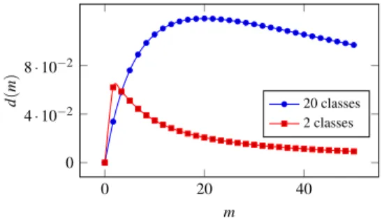
; if expectations of utilities are computed over a long enough number of bets, the expected utility produced by the two classifiers is the same. It also follows that increasingndelays the convergence of the expected utilities to the same value, as also shown in Fig.1.

Fig. 1. Functiond(m)forlogarithmicutility, under different number of classes.

8.2. Exponential utility

The exponential utility is u

(

x

)

:=

1

−

exp

(

−

ax

)

, where ais a coefficient of risk aversion. Noting thatu

(

x

)

=

−

a2exp

(

−

ax

)

, the second-order approximation yields:

u

(

E

[

rm

]

)

+

1 2u m n Var

(

rm

)

=

u _m n

−

1 2a 2_exp

₋

_am n m1 n 1

−

1 n

,

whence d

(

m

)

= −

1 2a 2_exp

₋

_am n m1 n 1

−

1 n

∝ −

exp

−

am n m

,

where the proportionality constant isa₂21_n1

−

1_n

>

0. We have d

(

m

)

=

exp

−

am n

·

am n

−

1

.

Functiond

(

m

)

has qualitatively the same behavior of the logarithmic case, but the inversion point is now located atm

=

n_a. Moreover, the difference between the expected utility of the two classifiers depends also on the risk-aversion coefficienta; higher risk aversion delays the convergence of the expected utilities, thus emphasizing the difference in favor of the vacuous on smallm.

9. Experiments

To experimentally assess the performance of a credal classifier, we need a utility function to be applied on top of discounted accuracy. Let us fix the utility of a correct and determinate classification asu

(

1

)

:=

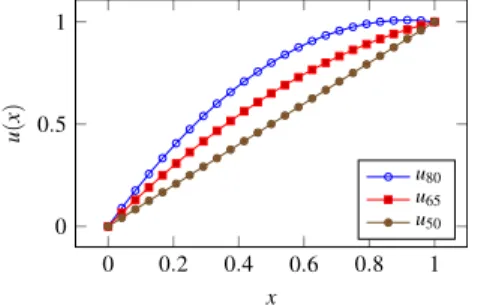
1 and the utility of a wrong classification

Fig. 2. The three quadratic utility functions obtained for different values ofu(0.5). The function corresponding to discounted accuracy isu50.

(determinate or indeterminate) asu

(

0

)

:=

0; this is consistent with the assumption that you are risk neutral in the scale of the original rewards.

Let us initially consider the case of a binary classification problem. To fully specify the utility function, we have to define the value ofu

(

0

.

5

)

. Withu

(

0

.

5

)

=

0

.

5, the utility leads to the standard discounted accuracy measure. Risk-aversion increases asu

(

0

.

5

)

increases. We assume that in case of risk aversion,u

(

0

.

5

)

can reasonably lie between 0.65 and 0.8; we callu65and u80the utility functions corresponding to these choices, andu50the one related to discounted accuracy.

In order to deal with classification problems with more than two classes, we adopt a quadratic utility function, which passes throughu

(

0

)

=

0

,

u

(

1

)

=

1, andu

(

0

.

5

)

=

0

.

65 oru

(

0

.

5

)

=

0

.

80. The two utility functions are:

u65

(

x

)

= −

1

.

2x2

+

2

.

2x

,

u80

(

x

)

= −

0

.

6x2

+

1

.

6x

,

wherexdenotes the discounted accuracy of the issued classification. These functions are shown in Fig.2. Note thatu80is

slightly greater than 1 for somexbetween 0.5 and 1; however, this part of the function is never used, as discounted accuracy cannot assume values between 0.5 and 1. This means that the range of values returned by all the functions will be

[

0

,

1

]

, which will allow us to interpret the resulting utility-discounted accuracies indeed as predictive accuracies (even though they are biased accuracies so as to take into account your personal preferences).

A well-known drawback of the quadratic utility function is that it models the risk aversion as increasing with wealth. Yet, at least under particular conditions, quadratic and exponential utility result in very similar choices [3]. Moreover, using quadratic utility has the advantage to make Eq. (1) an exact representation of the utility function, whose effects can then be interpreted very clearly as due to a compromise between increasing gain and reducing variability. We considered using the exponential utility too, but we eventually discarded it as it could not satisfactorily fit all the values we chose foru

(

0

.

5

)

.

9.1. NBC versus NCC

In this section we focus the comparison on two well-known classifiers: naive Bayes classifier (NBC [10]) as a representative of precise classifiers, and the naive credal classifier (NCC [25,26,6]). In particular, we compare the expected utility generated by NBC and NCC on the nextsinglebet, namely on a single instance.

9.1.1. Artificial data sets

In a first set of experiments, we generated artificial data sets consisting of binary class and 10 binary features; we set the marginal chances of classes as uniform, while we drew the conditional chances of the features under the constraint

|

θ

i1

−

θ

i2

| ≥

0

.

1

∀

i

,

j, where

θ

ijdenotes the chance of featureAito be in state

whenC

=

j; the constraint forced each

feature to be strongly dependent on the class. We drew

θ

80 times uniformly at random and we considered the sample sizes:s

∈ {

25

,

50

,

100

}

. We did not consider larger sample sizes, under which NCC would have been almost completely determinate, and thus not really different from NBC. For each pair

(θ,

s

)

we generated 50 training sets; we then evaluated the trained classifiers on a test set of 10000 instances. In the following, the instances indeterminately classified by NCC are referred to as thearea of ignorance. For each sample size, we thus perform 80 (#

(θ)

)

×

50 (trials)

=

4000 training/test experiments. In these experiments, we only consider theu65utility function.

As it can be seen in Fig.3, the discounted accuracy of NBC is higher than the discounted accuracy of NCC; this means that, on the area of ignorance, NBC is doing better than theK-random guesser, namely the classifier which picks the class at random from among those returned by NCC. Note that for NBC there is no distinction between accuracy and utility. However, NCC produces higher expected utility than NBC at each sample size, even under the conservative choiceu65.

9.1.2. Experiments with downsampling

We then performed some experiments on the kr-vs-kp data set from the UCI repository. It is a binary data set, in which the two classes are evenly distributed; it contains 36 binary features and 3200 instances. We downsampled the data set, generating training sets of sizes

∈ {

5

,

10

,

15

,

20

,

30

,

50

,

100

,

150

}

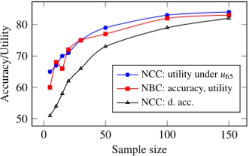
. For each sample size, we sampled 100 different training sets; the test set was given by the instances left in the original data set. Again, we considered the conservative choiceu65. The

Fig. 3. Experimental results with artificial data; each point shows the median over 4000 experiments, performed with the same sample sizes. For NBC, accuracy and utility coincide.

Fig. 4. Result of experiments with downsampling.

the discounted accuracy of NCC and the accuracy of NBC. For very small sample sizes, NCC is almost always indeterminate; in this case, its utility corresponds tou

(

0

.

5

)

and thus is 0.65; in the same situation NBC is only slightly better than random guessing. The expected utility of both NBC and NCC increases with the sample size; that of NCC remains however slightly superior. By adopting theu80function instead of theu65, the advantage of NBC would have obviously been more evident.

9.1.3. Experiments with real data sets

To get a more comprehensive picture of the performances of NBC and NCC, we performed experiments with 55 public data sets from the UCI repository; the number of classes varies from 2 to 26, the number of features from 2 to 36, the number of instances from 24 to more than 10000. We will consider this collection of data sets also in the next sections. On each data set, we performed ten runs of ten-fold cross validation. To compare two classifiers on thewholecollection of data sets,5 we used the Wilcoxon signed-rank test, as recommended by [8]. All tests are performed with

α

:=

0

.

05.

Since NCC operates only on discrete data, each data set has been discretized using the MDL-based discretization [12]; this approach determines for each feature variable the number of bins and the span of each bin, in a way which is optimal according to the minimum description length criterion. The discretization bins are thus learned from data; they are learned from the training set and applied unchanged to the test set.

Under the risk-neutral utility (i.e., discounted accuracy), the accuracy of NBC was higher than the discounted accuracy of NCC in 32 the data sets, while the converse held on 23 data sets. This difference in favor of NBC, as an aggregate measure over the 55 data sets, was statistically significant. This indicates that NBC most often performs better than theK-random guesser on the instances where NCC is indeterminate; surprisingly, it also happens to perform worse in several data sets. However, no significant difference was found underu65and underu80, when comparing the expected utility produced by

NCC and NBC over the collection of data sets. The expected utilities of NBC and NCC on each data set underu65andu80

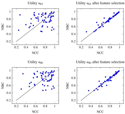
are compared in Fig.5(left column) through scatter plots. The straight line in the figures represents equal expected utility performance. Points above the line indicate cases where NBC outperformed NCC; conversely, points below the line indicate cases where NCC outperformed NBC. The plots show a slight increase of the expected utility of NCC as we move fromu65to u80, as expected.

The median accuracy of NBC was 82%, while the median expected utility of NCC vary from 75% under linear utility to 78% underu65to 81% underu80, suggesting that, as expected, NCC’s performance improves as we increase risk aversion. On 33

out of the 55 data sets, NCC had a determinacy higher than 90%, indicating that, in most of the data sets, NCC issued few indeterminate predictions. The median determinacy was 0.95.

NCC faces difficulties when the contingency table induced from a data set contains many zero counts, which causes NCC to be excessively indeterminate. Several such data sets are comprised in our collection. In these cases, restricting the credal set of NCC can largely increase the expected utility of NCC [4]; however, this is outside the scope of this paper.

5

This means that the possible significance of a comparison is related to the overall performance on the collection of data sets, rather than on a data set by data set basis.