Parallel Lossless Data Compression on the GPU

Title

Parallel Lossless Data Compression on the GPU

Permalink

Author

Publication Date

eScholarship.org Powered by the California Digital Library

RITESHA. PATEL

B.S. (University of California, Davis) 2010 THESIS

Submitted in partial satisfaction of the requirements for the degree of MASTER OFSCIENCE

in

Electrical and Computer Engineering in the

OFFICE OFGRADUATESTUDIES of the

UNIVERSITY OFCALIFORNIA DAVIS

Approved:

John D. Owens, Chair

Kent D. Wilken

Rajeevan Amirtharajah Committee in Charge

2012

-ii-List of Figures . . . v List of Tables . . . vi Abstract . . . vii Acknowledgments . . . viii 1 Introduction 1 1.1 Background . . . 1 1.2 Compression Pipeline . . . 2 1.3 Decompression Pipeline . . . 2 1.4 bzip2 Pipeline . . . 3 1.5 Challenges . . . 3 1.6 Contributions . . . 3 2 Compression Pipeline 5 2.1 Burrows-Wheeler Transform . . . 5

2.1.1 BWT with Merge Sort . . . 7

2.2 Move-to-Front Transform . . . 8

2.2.1 Parallel MTF Theory and Implementation . . . 9

2.3 Huffman Coding . . . 11 2.3.1 Histogram . . . 13 2.3.2 Huffman Tree . . . 13 2.3.3 Encoding . . . 13 3 Decompression 15 3.1 Huffman Decoding . . . 15 3.1.1 Parallel Decoding . . . 15

3.2 Reverse Move-to-Front Transform . . . 16

3.2.1 Parallel Reverse Move-to-Front Transform . . . 16

3.3 Reverse Burrows-Wheeler Transform . . . 18

3.3.1 Parallel Reverse Burrows-Wheeler Transform . . . 20

-iii-4.2 bzip2 Comparison . . . 24

4.2.1 Compression . . . 24

4.2.2 Decompression . . . 24

4.3 Memory Bandwidth . . . 25

4.4 Analysis of Kernel Performance . . . 25

4.4.1 Burrows-Wheeler Transform . . . 25

4.4.2 Reverse Burrows-Wheeler Transform . . . 27

4.4.3 Move-to-Front Transform . . . 29

4.4.4 Reverse Move-to-Front Transform . . . 30

4.4.5 Huffman Coding . . . 30 5 Discussion 32 5.1 Bottlenecks . . . 32 5.1.1 Compression . . . 32 5.1.2 Decompression . . . 34 5.2 Future Work . . . 35 6 Conclusion 37

-iv-2.1 Compression pipeline . . . 6

2.2 BWT example . . . 7

2.3 MTF example . . . 9

2.4 Parallel MTF algorithm . . . 12

2.5 Parallel reduction for Huffman tree . . . 14

3.1 Huffman decoding example . . . 16

3.2 Reverse-MTF example . . . 17

3.3 Reverse-BWT example . . . 19

3.4 Linked-list Traversal . . . 21

3.5 Parallel Reverse-BWT . . . 22

4.1 Required compression rate . . . 26

4.2 PCI-Express and GPU memory bandwidth over time . . . 26

4.3 BWT ties analysis . . . 28

4.4 Serial MTF vs. parallel scan-based MTF . . . 28

4.5 MTF local scan performance . . . 29

4.6 Serial reverse-MTF vs. parallel scan-based reverse-MTF . . . 31

4.7 Runtime breakdown of Huffman coding . . . 31

-v-4.1 GPU vs. bzip2 compression . . . 23 4.2 GPU vs. bzip2 decompression . . . 24 4.3 Average reverse-BWT rates . . . 27

-vi-Parallel Lossless Data Compression on the GPU

In this thesis we present parallel algorithms and implementations of a bzip2-like lossless data compression scheme for GPU architectures. Our approach parallelizes three main stages in the bzip2 compression/decompression pipeline: Burrows-Wheeler transform (BWT), move-to-front transform (MTF), and Huffman coding. In particular, we utilize a two-level hierarchical sort for the forward-BWT, invent a novel parallel reverse-BWT algorithm, design a novel scan-based parallel MTF and reverse-MTF algorithm, implement parallel Huffman encoding/decoding, and implement a parallel reduction scheme to build the Huffman tree. For each algorithm, we per-form detailed perper-formance analysis, discuss its strengths and weaknesses, and suggest future directions for improvements. Overall, our GPU implementation of the compression pipeline is dominated by BWT performance and is 2.78×slower than bzip2, with BWT and MTF+Huffman respectively 2.89× and 1.34× slower on average. Our overall GPU decompression runtime is distributed more evenly and is 1.2× faster, with reverse-BWT 2.45× faster and reverse-MTF+Huffman 1.83×slower than bzip2.

-vii-This work would not have been possible without the support and care of the people around me. First and foremost, I’d like to thank my advisor, John Owens, who gave me the opportunity to be a part of his wonderful and talented research team. It’s tough to put into words how thankful I am to someone who has helped shape my career. In two years, John has given me more confidence in myself and in my work than I’ve ever had—inspiring me to complete a publication, and recommending me to top industry leaders for internships and full-time positions. I am certain that without his encouragement and support, I would not be the student I am today. Leaving “owensgroup” is bittersweet and I hope to continue to collaborate with John and his team in the future.

Next, I would like thank Professor Kent Wilken and Professor Rajeevan Amirtharajah for reviewing my thesis and providing valuable feedback and comments along the way.

I’ve had the pleasure of working with some of the most talented individuals I know. This includes Anjul Patney, Stanley Tzeng, Andrew Davidson, Jason Mak, Yao Zhang, Afton Geil, Yangzihao Wang, Calina Copos, Jeff Stuart, and Shubhabrata Sengupta. In particular, I was fortunate to work on my first publication with Yao Zhang, Andrew Davidson, and Jason Mak. I’d also like to give many thanks to Anjul Patney and Stanley Tzeng for their guidance throughout this process.

Next, I would to thank Adam Herr and Allen Hux for offering me a summer internship opportunity at Intel while allowing me to continue my research along the way.

I’ve been blessed with the support and motivation I’ve received from my family and friends. Many thanks to my sister-in-law, Divya Patel, for taking the time to read over my work and provide valuable feedback. I thank my girlfriend, Preya Sheth, for her encouragement and sup-port throughout this study. She has truly been a great friend over the years. Finally, I thank my beloved parents and my brother. My parents have always provided unconditional financial and emotional support and I can not thank them enough. My dad, Ashok Patel, has always been the inspiration for my work. I wouldn’t be the man I am today without his encouragement and drive. My mother, Usha Patel, has taught me invaluable life lessons that have molded me as a person. Her hard-work and dedication is unparalleled. Finally, to my brother, Shyam Patel, for always being a helping hand. I could not be more lucky to have such a caring brother.

-viii-Chapter 1

Introduction

1.1

Background

Data compression is a crucial part in data storage and distributed systems that require large amounts of data transmission. It aims to increase effective data density by reducing redundant data and minimizing data communication. Data compression has been frequently implemented in two ways: (1) software compression running on a general-purpose CPU; (2) hardware com-pression that requires specialized hardware equipment. Hardware comcom-pression is considerably faster than software, but it is more expensive and not configurable. Software compression is low-cost, easily accessible, and much more flexible than hardware compression. However, it adds additional burden to the host processor and can degrade the performance of the host dur-ing heavy usage. In this work, we lighten this burden by utilizdur-ing the graphics processdur-ing unit (GPU) as a compression/decompression coprocessor. This is a challenge because the GPU is a massively parallel architecture and common compression algorithms are not parallel-friendly.

We implement parallel data compression and decompression algorithms on a GPU. We study the challenges of parallelizing compression algorithms, the potential performance gains offered by the GPU, and the limitations of the GPU that prevent optimal speed-up. In addition, we see many practical motivations for this research. Applications that have large data storage demands but run in memory-limited environments can benefit from high-performance compression algo-rithms. The same is true for systems where performance is bottlenecked by data communication. These distributed systems, which include high-performance multi-node clusters, are willing to tolerate additional computation to minimize the data sent across bandwidth-saturated network connections. In both cases, a GPU can serve as a compression/decompression coprocessor

op-erating asynchronously with the CPU to relieve the computational demands of the CPU and support efficient data compression with minimal overhead.

The GPU is a highly parallel architecture that is well-suited for large-scale file processing. In addition to providing massive parallelism with its numerous processors, the GPU benefits the performance of our parallel compression through its memory hierarchy. A large global memory residing on the device allows us to create an efficient implementation of a compression pipeline found in similar CPU-based applications, including bzip2. The data output by one stage of compression remains in GPU memory and serves as input to the next stage. To maintain high performance within the algorithms of each stage, we use fast GPU shared memory to cache partial file contents and associated data structures residing as a whole in slower global memory. Our algorithms also benefit from the atomic primitives provided in CUDA [1]. These atomic operations assist in the development of merge routines needed by our algorithms.

1.2

Compression Pipeline

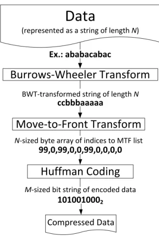
We implement our compression application as a series of three stages. Our compression pipeline, similar to the one used by bzip2, executes the Burrows-Wheeler transform (BWT), the move-to-front transform (MTF), and ends with Huffman coding. The BWT inputs the text string to compress, then outputs an equally-sized BWT-transformed string; MTF outputs an array of indices; and the Huffman stage outputs the Huffman tree and the Huffman encoding of this list. The BWT and MTF apply reversible transformations to the file contents to increase the effectiveness of Huffman coding, which performs the actual compression. Each algorithm is described in greater detail in Chapter 2. This execution model is well-suited to CUDA, where each stage is implemented as a set of CUDA kernels, and the output from kernels are provided as input to other kernels.

1.3

Decompression Pipeline

The decompression pipeline works in the reverse order, starting with Huffman decoding, fol-lowed by the reverse move-to-front transform, and ending with the reverse Burrows-Wheeler transform. The Huffman decoding stage starts by rebuilding the Huffman tree using data stored in the encoded file. We generate the same Huffman codes by using the same tree generation algorithm that we use during encoding. Next, we perform the reverse-MTF transform using the same MTF list we started with in the forward MTF transform i.e. 0,1,2, . . . ,255. The final

step in the decompression pipeline is the reverse BWT. Similar to the compression stages, we execute each of the decompression stages using parallel algorithms implemented using CUDA. Each decompression algorithm is described in detail in Chapter 3.

1.4

bzip2 Pipeline

Our implementation is not compliant with bzip2 since bzip2 uses additional compression tech-niques in its pipeline. We address the primary research challenges of implementing both direc-tions of the Burrows-Wheeler transform, move-to-front transform, and Huffman coding. bzip2 implements run-length encoding in which runs of data are stores as as single data value. The bzip2 application implements a modified form of Huffman coding that uses multiple Huffman tables [2]. The implementation creates 2 to 6 Huffman tables and selects the most optimal table for every block of 50 characters. This approach can potentially result in higher compression ratios. For simplicity and performance, we do not employ this technique in our implementation. Section 5.2 discusses how we plan to address these differences.

1.5

Challenges

Although Gilchrist presents a multi-threaded version of bzip2 that uses the Pthreads library [3], the challenges of mapping bzip2 to the GPU lie not only in the implementation, but more funda-mentally, in the algorithms. bzip2’s data locality is poorly suited to the memory hierarchy of the GPU. The BWT implementation in bzip2 is based on radix sort and quicksort, which together require substantial global communication. The reverse BWT algorithm is highly serial and simi-lar to traversing a linked list. The traditional MTF and reverse-MTF algorithms are strictly serial with a character-by-character dependency.

1.6

Contributions

We make the following contributions in the paper. First, we design parallel algorithms and GPU implementations for three major stages of bzip2: BWT, MTF, and Huffman coding. We re-design BWT using a hierarchical merge sort that sorts locally and globally. The use of a local sort distributes the workload to the GPU cores and minimizes the global communication. We present a novel reverse-BWT algorithm in which the output is able to be computed in parallel. We invent novel scan-based MTF and reverse-MTF algorithms that break the input MTF list into small chunks and processes them in parallel. We also build the Huffman tree using a parallel

reduction scheme. Next, we conduct a comprehensive performance analysis, which reveals the strengths and weaknesses of our parallel algorithms and implementations, and further suggest future directions for improvements. Our implementation enables the GPU to become a com-pression/decompression coprocessor, which lightens the processing burden of the CPU by using idle GPU cycles. We also assess the viability of using compression to trade computation for communication over the PCI-Express bus.

Chapter 2

Compression Pipeline

Our compression pipeline consists of three main stages as shown in Figure 2.1.

Burrows-Wheeler Transform (BWT) is the first stage in our compression pipeline. The BWT is a reversible transformation that rearranges the characters of a block of data using sorting. The result of the BWT is a block of data containing many repeated characters.

Move-to-Front Transform (MTF) is the second stage in our pipeline. The MTF improves the effectiveness of entropy encoding by transforming a block of data containing long sequences of identical characters by small integers, i.e. 0’s, 1’s, etc.

Huffman Coding is the third and final stage in our pipeline. Huffman coding is an entropy encoding algorithm that uses variable-length codes to encode data. It works by generating shorter codes for symbols that occur more frequently, while generating longer codes for symbols that occur less frequently.

2.1

Burrows-Wheeler Transform

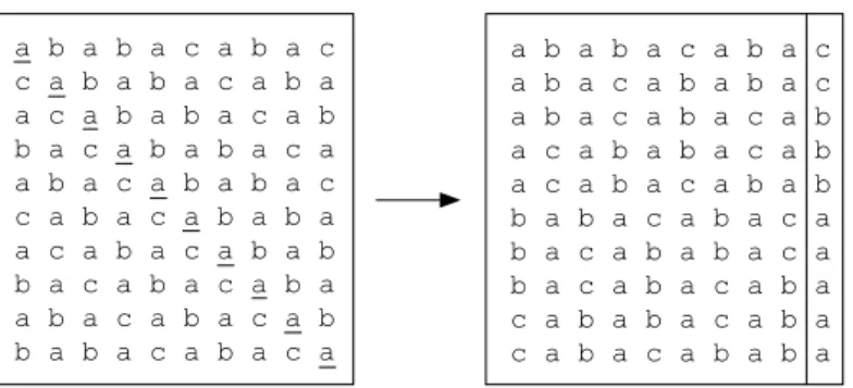
The first stage in the compression pipeline, an algorithm introduced by Burrows and Wheeler [4], does not itself perform compression but applies a reversible reordering to a string of text to make it easier to compress. The Burrows-Wheeler transform (BWT) begins by producing a list of strings consisting of all cyclical rotations of the original string. This list is then sorted, and the last character of each rotation forms the transformed string. Figure 2.2 shows this process being applied to the string “ababacabac”, where the cyclical rotations of the string are placed into rows of a block and sorted from top to bottom. The transformed string is formed by simply taking the

Data

(represented as a string of length N)

Burrows-Wheeler Transform

Compressed Data

Move-to-Front Transform

Huffman Coding

Ex.: ababacabac

ccbbbaaaaa

99,0,99,0,0,99,0,0,0,0

101001000

N-sized byte array of indices to MTF list

M-sized bit string of encoded data BWT-transformed string of length N

Figure 2.1:Our compression pipeline consists of three stages: (1) Burrows-Wheeler Transform; (2) Move-to-Front Transform; (3) Huffman Coding.

last column of the block. In order for the transform to be reversible, the index where the original string was sorted must also be stored.

The new string produced by BWT tends to have many runs of repeated characters, which bodes well for compression. To explain why their algorithm works, Burrows and Wheeler use an example featuring the common English word “the”, and assume an input string containing many instances of “the”. When the list of rotations of the input is sorted, all the rotations starting with “he” will sort together, and a large proportion of them are likely to end in ‘t’ [4]. In general, if the original string has several substrings that occur often, then the transformed string will have several places where a single character is repeated multiple times in a row. To be feasible for compression, BWT has another important property—reversibility. Burrows and Wheeler also describe the process to reconstruct the original string [4].

a b a b a c a b a c a b a c a b a b a c a b a c a b a c a b a c a b a b a c a b a c a b a c a b a b b a b a c a b a c a b a c a b a b a c a b a c a b a c a b a c a b a b a c a b a c a b a c a b a b a a b a b a c a b a c c a b a b a c a b a a c a b a b a c a b b a c a b a b a c a a b a c a b a b a c c a b a c a b a b a a c a b a c a b a b b a c a b a c a b a a b a c a b a c a b b a b a c a b a c a

Figure 2.2:BWT permutes the string “ababacabac” by sorting its cyclical rotations in a block. The last column produces the output “ccbbbaaaaa”, which has runs of repeated characters. The original string is shown in bold. Since the original string was sorted to the first position, the index stored is 0.

expensive stage. Sorting in BWT is a specialized case of string sort. Since the input strings are merely rotations of the original string, they all consist of the same characters and have the same length. Therefore, only the original string needs to be stored, while the rotations are represented by pointers or indices into a memory buffer.

The original serial implementation of BWT uses radix sort to sort the strings based on their first two characters followed by quicksort to further sort groups of strings that match at their first two characters [4]. Seward [5] shows the complexity of this algorithm to beO(A·nlogn), whereAis the average number of symbols per rotation that must be compared to verify that the rotations are in order.

Sorting has been extensively studied on the GPU, but not in the context of variable-length keys (such as strings) and not in the context of very long, fixed-length keys (such as the million-character strings required for BWT). Two of the major challenges are the need to store the keys in global memory because of their length and the complexity and irregularity of a comparison function to compare two long strings.

2.1.1 BWT with Merge Sort

In our GPU implementation of BWT, we leverage a string sorting algorithm based on merge sort [6]. The algorithm uses a hierarchical approach to maximize parallelism during each stage. Starting at the most fine-grained level, each thread sorts 8 elements with bitonic sort. Next, the algorithm merges the sorted sequences within each block. In the last stage, a global inter-block merge is performed, in whichbblocks are merged in log₂bsteps. In the later inter-block merges,

only a small number of large unmerged sequences remain. These sequences are partitioned so that multiple blocks can participate in merging them.

Since we are sorting rotations of a single string, we use the first four characters of each rotation as the sort key. The corresponding value of each key is the index where the rotation begins in the input string. The input string is long and must be stored in global memory, while the sort keys are cached in registers and shared memory. When two keys are compared and found equal, a thread continually fetches the next four characters from global memory until the tie can be broken. Encountering many ties causes frequent access to global memory while incurring large thread divergence. This is especially the case for an input string with long runs of repeating characters. We discuss our experimental results in more detail in Section 4.4.1. After sorting completes, we take the last characters of each string to create the final output of BWT: a permutation of the input string that we store in global memory.

No previous GPU work implements the full BWT, primarily (we believe) because of the prior lack of any efficient GPU-based string sort. One implementation alternative is to substitute a simpler operation than BWT. The Schindler Transform (STX), instead of performing a full sort on the rotated input string, sorts strings by the firstX characters. This is less effective than a full BWT, but is computationally much cheaper, and can be easily implemented with a radix sort [7].

2.2

Move-to-Front Transform

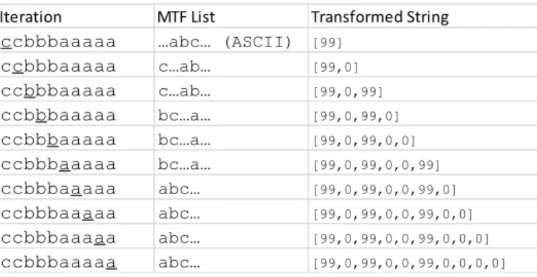
The move-to-front transform (MTF) improves the effectiveness of entropy encoding algorithms [8], of which Huffman encoding is one of the most common. When applied to a string that has been transformed by BWT, MTF tends to output a new sequence of small numbers with more repeats. MTF replaces each symbol in a stream of data with its corresponding position in a list of recently used symbols. MTF takes advantage of repeated characters by keeping recently used characters at the front of the list. Figure 2.3 shows the application of MTF to the string “ccbb-baaaaa” produced by BWT from an earlier example, where the list of recent symbols is initialized as the list of all ASCII characters. Although the output of MTF stores the indices of a list, it is essentially a byte array with the same size as the input string.

Algorithm 1 shows pseudo-code for the serial MTF algorithm. At first glance, this algorithm appears to be completely serial; exploiting parallelism in MTF is a challenge because determin-ing the index for a given symbol is dependent on the MTF list that results from processdetermin-ing all

Algorithm 1Serial Move-to-Front Transform

Input:A char-arraymtfIn.

Output:A char-arraymtfOut. 1: {Generate Initial MTF List} 2: fori=0→255do

3: mtfList[i]=i

4: for j=0→sizeof(mtfIn)−1do 5: K=mtfIn[j]

6: mtfOut[j]=K’s position inmtfList 7: MoveKto front ofmtfList

Iteration MTF List Transformed String

ccbbbaaaaa …abc… (ASCII) [99]

ccbbbaaaaa c…ab… [99,0] ccbbbaaaaa c…ab… [99,0,99] ccbbbaaaaa bc…a… [99,0,99,0] ccbbbaaaaa bc…a… [99,0,99,0,0] ccbbbaaaaa bc…a… [99,0,99,0,0,99] ccbbbaaaaa abc… [99,0,99,0,0,99,0] ccbbbaaaaa abc… [99,0,99,0,0,99,0,0] ccbbbaaaaa abc… [99,0,99,0,0,99,0,0,0] ccbbbaaaaa abc… [99,0,99,0,0,99,0,0,0,0]

Figure 2.3:The MTF transform is applied to a string produced by BWT, “cccbbbaaaaa”. In the first step, the character ‘c’ is found at index 99 of the initial MTF list (the ASCII list). Therefore, the first value of the output is byte 99. The character ‘c’ is then moved to the front of the list and now has index 0. At the end of the transform, the resulting byte array has a high occurrence of 0’s, which is beneficial for entropy encoding.

prior symbols. In our approach, we implement MTF as a parallel operation, one that can be expressed as an instance of the scan primitive [9]. We believe that this parallelization strategy is a new one for the MTF algorithm.

2.2.1 Parallel MTF Theory and Implementation

Each step in MTF encodes a single character by finding that character in the MTF list, recording its index, and then moving the character to the front of the list. The algorithm is thus apparently serial. We break this serial pattern with two insights:

1. Given a substringsof characters located somewhere within the input string, and without knowing anything about the rest of the string either before or following, we can generate a

partial MTF listthat computes the partial MTF forsthat only contains the characters that appear ins(Algorithm 2).

2. We can efficiently combine two partial MTF lists for two adjacent substrings to create a partial MTF list that represents the concatenation of the two substrings (Algorithm 3). We combine these two insights in our parallel divide-and-conquer implementation. We di-vide the input strings into small 64-character substrings and assign each substring to a thread. We then compute a partial MTF list for each substring per thread, then recursively merge those partial MTF lists together to form the final MTF list. We now take a closer look at the two algorithms.

Algorithm 2MTF Per Thread

Input:A char-arraymtfIn.

Output:A char-arraymyMtfList. 1: Index= 0

2: J= Number of elements per substring

3: fori= ((threadID+1)×J)−1→threadID×Jdo 4: mtfVal=mtfIn[i]

5: ifmtfValdoes NOT exist inmyMtfListthen 6: myMtfList[Index++]=mtfVal

Algorithm 2 describes how we generate a partial MTF list for a substring s of length n. In this computation, we need only keep track of the characters in s. For example, the partial MTF list for “dead” is [d,a,e], and the partial list for “beef” is [f,e,b]. We note that the partial MTF list is simply the ordering of characters from most recently seen to least recently seen. Our implementation runs serially within each thread, walkings from its last element to its first element and recording the first appearance of each character ins. Our per-thread implementation is SIMD-parallel so it runs efficiently across threads. Because all computation occurs internal to a thread, we benefit from fully utilizing the registers in each thread processor, andnshould be as large as possible without exhausting the hardware resources within a thread processor. The output list has a maximum size ofnor the number of possible unique characters in a string (256 for 8-bit byte-encoded strings), whichever is smaller. After each thread computes its initial MTF list, there will beN/nindependent, partial MTF lists, whereNis the length of our input string.

To reduce two successive partial MTF lists into one partial MTF list, we use theAppendUnique()

function shown in Algorithm 3. This function takes characters from the first list that are absent in the second list and appends them in order to the end of the second list. For example, applying

AppendUnique()to the two lists [d,a,e] for the string “dead” and [f,e,b] for the string “beef” re-sults in the list [f,e,b,d,a]. This new list orders the characters of the combined string “deadbeef”

Algorithm 3AppendUnique()

Input:Two MTF listsListn,Listn−1. Output:One MTF listListn.

1: j= sizeof(Listn)

2: fori=0→sizeof(Listn−1)−1do 3: K=Listn−1[i]

4: ifKdoes NOT exist inListnthen

5: Listn[j++]=K

from most recently seen to least recently seen. Note that this merge operation only depends on the size of the partial lists (which never exceed 256 elements for byte-encoded strings), not the size of the substrings.

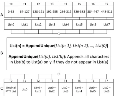
To optimize our scan-based MTF for the GPU, we adapt our implementation to the CUDA programming model. First, we perform a parallel reduction within each thread-block and store the resulting MTF lists in global memory. During this process, we store and access each thread’s partial MTF list in shared memory. Next, we use the MTF lists resulting from the intra-block reductions to compute a global block-wise scan. The result for each block will be used by the threads of the subsequent block to compute their final outputs independent of threads in other blocks. In this final step, each thread-block executes scan using the initial, partial lists stored in shared memory and the lists outputted by the block-wise scan stored in global memory. With the scan complete, each thread replaces symbols in parallel using its partial MTF list outputted by scan, which is the state of the MTF list after processing prior characters. Figure 2.4 shows a high-level view of our algorithm.

MTF can be formally expressed as an exclusive scan computation, an operation well-suited for GPU architectures [9]. Scan is defined by three entities: an input datatype, a binary asso-ciative operation, and an identity element. Our datatype is a partial MTF list, our operator is the functionAppendUnique(), and our identity is the initial MTF list (for a byte string, simply the 256-element arrayawherea[i] =i). It is likely that the persistent-thread-based GPU scan formulation of Merrill and Grimshaw [10] would be a good match for computing the MTF on the GPU.

2.3

Huffman Coding

Huffman coding is an entropy-encoding algorithm used in data compression [11]. The algorithm replaces each input symbol with a variable-length bit code, where the length of the code is

448-511 384-447 320-383 256-319 192-255 128-191 64-127 0-63 List7 List6 List5 List4 List3 List2 List1 List0 T7 T6 T5 T4 T3 T2 T1 T0 List0 – List6 List0 – List5 List0 – List4 List0 – List3 List0 – List2 List0 – List1 List0 Original MTF List

List(n) = AppendUnique(List(n-1), List(n-2), …, List(0)) AppendUnique(List(a), List(b)): Appends all characters

in List(b) to List(a) only if they do not appear in List(a)

T7 T6 T5 T4 T3 T2 T1 T0 A B C

Figure 2.4: Parallel MTF steps: A) Each thread computes a partial MTF list for 64 characters (Algorithm 2). B) An exclusive scan executes in parallel with AppendUnique() as the scan oper-ator (Algorithm 3). C) The scan output for each thread holds the state of the MTF list after all prior characters have been processed. Each thread is able to independently compute a part of the MTF transform output.

determined by the symbol’s frequency of occurrence. There are three main computational stages in Huffman coding: (1) generating the character histogram, (2) building the Huffman tree, and (3) encoding data.

First, the algorithm generates a histogram that stores the frequency of each character in the data. Next, we build the Huffman tree as a binary tree from the bottom up using the histogram. The process works as follows. At each step, the two least-frequent entries are removed from the histogram and joined via a new parent node, which is inserted into the histogram with a frequency equal to the sum of the frequencies of its two children. This step is repeated until one entry remains in the histogram, which becomes the root of the Huffman tree.

Once the tree is built, each character is represented by a leaf in the tree, with less-frequent characters at a deeper level in the tree. The code for each character is determined by traversing the path from the root of the tree to the leaf representing that character. Starting with an empty code, a zero bit is appended to the code each time a left branch is taken, and a one bit is appended each time a right branch is taken. Characters that appear more frequently have shorter codes, and

full optimality is achieved when the number of bits used for each character is proportional to the logarithm of the character’s fraction of occurrence. The codes generated by Huffman coding are also known as “prefix codes”, because the code for one symbol is never a prefix of a code representing any other symbol, thus avoiding ambiguity that can result from having variable-length codes. Finally, during the encoding process, each character is replaced with its assigned bit code.

In trying to parallelize the construction of the Huffman tree, we note that as nodes are added and joined, the histogram changes, so we cannot create nodes in parallel. Instead, we perform the search for the two least-frequent histogram entries in parallel using a reduction scheme. Parallelizing the encoding stage is difficult because each Huffman code is a variable-length bit code, so the location to write the code in the compressed data is dependent on all prior codes. In addition, variable-length bit codes can cross byte boundaries, which complicates partitioning the computation. To perform data encoding in parallel, we use an approach that encodes into variable-length, byte-aligned bit arrays.

2.3.1 Histogram

To create our histogram, we use an algorithm presented by Brown et al. that builds 256-entry per-thread histograms in shared memory and then combines them to form a thread-block his-togram [12]. We compute the final global hishis-togram using one thread-block.

2.3.2 Huffman Tree

We use a parallel search algorithm to find the two least-frequent values in the histogram. Our algorithm, shown in Figure 2.5, can be expressed as a parallel reduction, where each thread searches four elements at a time. Our reduce operator is a function that selects the two least-frequent values out of four. Each search completes in log₂n−1 stages, wherenis the number of entries remaining in the histogram.

2.3.3 Encoding

We derive our GPU implementation for Huffman encoding from a prior work by Cloud et al. [13], who describe an encoding scheme that packs Huffman codes into variable-length, byte-aligned bit arrays but do not give specific details for their implementation in CUDA. Our implementation works in the following way. We use 128 threads per thread-block and assign 4096 codes to each block, thereby giving each thread 32 codes to write in serial. Similar to Cloud et al., we

byte-0 1 2 3 4 5 6 7 (X,Y) = 2-Min(0,1,2,3) (Z,W) = 2-Min(4,5,6,7) (Min1,Min2) = 2-Min(X,Y,Z,W)

Figure 2.5: We use a parallel reduction to find the two lowest occurrences. This technique is used in the building of the Huffman tree.

align the bit array written by each parallel processor, or each thread-block in our case, by padding the end with zeroes so that we do not have to handle codes crossing byte boundaries across blocks and so that we can later decode in parallel. We also save the size of each bit array for decoding purposes. To encode variable-length codes in parallel, each block needs the correct byte offset to write its bit array, and each thread within a block needs the correct bit offset to write its bit sub-array (we handle codes crossing byte boundaries across threads). To calculate these offsets, we use a parallel scan across blocks and across threads within each block, where the scan operator sums bit array sizes for blocks and bit sub-array sizes for threads. After encoding completes, our final output is the compressed data, which stores the Huffman tree, the sizes of the bit arrays, and the bit arrays themselves interleaved with small amounts of padding.

Chapter 3

Decompression

The decompression pipeline consists of three stages: (1) Huffman decoding; (2) Reverse move-to-front transform; (3) Reverse Burrows-Wheeler transform. The reverBWT is highly se-rial and similar to traversing a linked list. Like the MTF, the reverse-MTF is strictly with a character-by-character dependency. Decompression works in the reverse order of our compres-sion pipeline, therefore, we will describe these stages starting with Huffman decoding.

3.1

Huffman Decoding

The Huffman decoding stage first builds the Huffman tree using the histogram stored in the encoded file. Once the tree is built, decoding is a straightforward algorithm that processes the data stream one bit at a time. To decode, we traverse the Huffman tree starting from the root. We take the left branch when a zero is encountered and the right branch when a one is encountered. When we reach a leaf, we write the uncompressed character represented by the leaf and restart our traversal at the root. Figure 3.1 shows an example of how decoding works, given a bit array and a Huffman tree.

3.1.1 Parallel Decoding

We perform the Huffman tree building on the CPU, as it is a highly serial algorithm and is not well suited for the GPU. In order to perform decoding in parallel, we assign each bit array to a thread so that each thread is responsible for writing 4096 uncompressed characters. By using CUDA’s vector type (uchar4), each thread is able to execute one write operation for every four characters decoded, decreasing the total number of global memory write operations. Although this simple approach uses less parallelism than our encoding implementation, we do not deter-mine this to be a performance issue because decoding, unlike encoding, does not require the extra

F 0 1 H U 0 1 Parent Codes H: 00 U: 01 F: 1 Encoded Data: 000111 Decoded Data: HUFF

Figure 3.1: Huffman decoding works by processing one bit at a time in the encoded data and traversing the Huffman tree until it reaches a leaf node. Once a character is decoded, traversal of the tree continues starting at the parent.

scan operations and bitwise operations needed to support writing variable-length data-types.

3.2

Reverse Move-to-Front Transform

The reverse-MTF transform, shown in Algorithm 4, restores the original sequence by taking the first index from the encoded sequence and outputting the symbol found at that index in the initial MTF list. The symbol is moved to the front of the MTF list, and the process is repeated for all subsequent indices stored in the encoded sequence. Figure 3.2 shows the application of the reverse-MTF to the sequence “99,0,99,0,0,99,0,0,0,0” produced by the forward MTF from an earlier example (Figure 2.3). Since the input sequence of characters are used as indices to find the corresponding output symbol in the MTF list, decoding can benefit from use of a linked-list to efficiently “move” nodes to the front of the list.

Like MTF, reverse-MTF appears to be a highly serial algorithm because we cannot restore an original symbol without knowing the MTF list that results from restoring all prior symbols. In parallelizing the reverse-MTF, we use a similar scan-based approach, in which the intermediate data is an altered MTF list and the operator is a permutation of a MTF list. We believe this parallelization strategy is a new one for the reverse-MTF algorithm.

3.2.1 Parallel Reverse Move-to-Front Transform

Each output of the reverse-MTF transform is dependent on the status of the MTF list at its index, making the reverse-MTF a highly serial problem. The goal of our parallel reverse-MTF algorithm is the same as our parallel MTF: Generaten MTF lists forndifferent indices in the input,nbeing the total number of threads. This allows each thread to compute a part of the MTF

Iteration MTF List Transformed String [99,0,99,0,0,99,0,0,0,0] …abc… (ASCII) c [99,0,99,0,0,99,0,0,0,0] c…ab… cc [99,0,99,0,0,99,0,0,0,0] c…ab… ccb [99,0,99,0,0,99,0,0,0,0] bc…a… ccbb [99,0,99,0,0,99,0,0,0,0] bc…a… ccbbb [99,0,99,0,0,99,0,0,0,0] bc…a… ccbbba [99,0,99,0,0,99,0,0,0,0] abc… ccbbbaa [99,0,99,0,0,99,0,0,0,0] abc… ccbbbaaa [99,0,99,0,0,99,0,0,0,0] abc… ccbbbaaaa [99,0,99,0,0,99,0,0,0,0] abc… ccbbbaaaaa

Figure 3.2: The reverse-MTF transform is applied to the sequence “99,0,99,0,0,99,0,0,0,0”. In the first step, the character ‘c’ is found at index 99 of the initial MTF list (the ASCII list). Therefore, the first value of the output is byte ‘c’. The character present at index 99, ‘c’, is then moved to the front of the MTF list. This process is repeated until all characters are decoded. Algorithm 4Serial Reverse Move-to-Front Transform

Input:A char-arraymtfRevIn.

Output:A char-arraymtfRevOut. 1: {Generate Initial MTF List} 2: fori= 0→255do

3: mtfList[i] =i

4: forj= 0→sizeof(mtfRevIn)-1do 5: K=mtfRevIn[j]

6: mtfRevOut[j] =mtfList[K]

7: MovemtfList[K] to front ofmtfList

output in parallel. Similar to the parallel MTF, we can achieve this with two observations: 1. Given a substringsof characters located somewhere within the input string, and without

knowing anything about the rest of the string either before or following, we can generate apartial MTF listthat computes the partial reverse-MTF fors(Algorithm 5).

2. We can combine two partial reverse-MTF lists for two adjacent sub-strings to create a partial MTF list using Algorithm 6.

As before, we use these two algorithms as the core in our parallel divide-and-conquer imple-mentation. We divide the input string into the same size (64-character) substrings as we did with the parallel MTF and assign each substring to a thread. We then compute the MTF list for each substring per thread, then recursively “merge” those partial MTF lists together to form the final MTF list. We now look at each algorithm in greater detail.

Algorithm 5Reverse MTF Operation Per Thread

Input:A char-arraymtfRevIn.

Output:A char-arraymyMtfList. 1: {Initialize MTF List} 2: fori=0→255do 3: myMtfList[i]=i

4: J= Number of elements per substring

5: fori= (threadID×J)→((threadID+1)×J)−1do 6: K=mtfRevIn[i]

7: MovemyMtfList[K]to front ofmyMtfList

Algorithm 5 is a simple reverse-MTF implementation computed by each thread. In this case, we only care about the status of each MTF list, therefore, we only move the indexed symbols to the front of the list and do not output them as we would in a serial implementation.

Algorithm 6Reverse-MTF List Scan Operator

Input:Two Reverse-MTF listsListn,Listn−1. Output:One Reverse-MTF listListn.

1: fori=0→255do 2: K=Listn[i]

3: Listn[i]=Listn−1[K]

Like the MTF, the reverse-MTF can be expressed as an exclusive scan computation, where the datatype is a partial MTF list computed using Algorithm 5, the operator is the function described in Algorithm 6, and the identity is the initial MTF list. Our operator (Algorithm 6) works by reducing two adjacent MTF lists into one MTF list. The function uses each value in the latter list to index into the previous list and replaces this value by the index value in the previous list. For example, applying our operator to two adjacent MTF lists [0,2,1,3,4] (generated from [2,1,0,0]) and [1,0,4,2,3] (generated from [4,1,0,2]) results in the MTF list [2,0,4,1,3]. This is the resulting MTF list when computing the reverse-MTF of [2,1,0,0,4,1,0,2].

We adapt a similar CUDA programming model for the parallel reverse-MTF implementation as we did for the parallel MTF described in Section 2.2.1.

3.3

Reverse Burrows-Wheeler Transform

The last stage in our decompression pipeline is the reverse Burrows-Wheeler transform. We start with a stringLcomposed of the last column of characters produced from the sorted cyclical rotations of the input to the BWT. We use an index integerithat represents the position of the

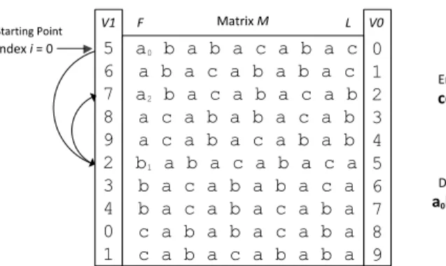
a0 b a b a c a b a c a b a c a b a b a c a2 b a c a b a c a b a c a b a b a c a b a c a b a c a b a b b1 a b a c a b a c a b a c a b a b a c a b a c a b a c a b a c a b a b a c a b a c a b a c a b a b a 0 1 2 3 4 5 6 7 8 9 5 6 7 8 9 2 3 4 0 1 Decoded String a0b1a2bacabac Encoded String ccbbbaaaaa L Matrix M V0 F V1 Index i =0 Starting Point

Figure 3.3: This figure shows the application of the reverse-BWT transformation to the string “ccbbbaaaaa” with index i = 0. First, we perform a key-value sort using column L as the keys and column V0 as the values. This results in columns F (sorted keys) and V1. Then, using index i = 0, we are able to determine the first character in the decoded sequence to be ‘a’. We then move the index to 5 and decode the next character to be ‘b’. We repeat this process until all characters are decoded.

original input within the sorted rotations. The index is used as a starting point; it tells us the value of the last character in the original string. We will now show how the index can be used to decode starting with the first character.

The first step in computing the reverse-BWT is to compute stringsFandV1from the sorted cyclical rotations in the BWT, as shown in Figure 3.3. StringF represents the first column of the sorted BWT rotations. It tells us the character of each neighboring element of string L. The reverse-BWT is similar to linked-list ranking. The index integerirepresents the head node pointer. StringV1 represents thenextpointer in our linked-list traversal process. We compute

F and V1 by performing a key-value sort using L as the keys and string V0 in Figure 3.3 as the values. We then useFandV1to compute the reversed-BWT. We first decode the character present atF[i]. In the example shown in Figure 3.3, the first character decoded is an ‘a’. We note that this is the same ‘a’ corresponding to the first occurring ‘a’ in arrayL; they share the same value of 5. Next, we perform the transformationi←V1[i]. In the example shown in Figure 3.3 the current valueV1[i] is 5. Therefore, we move the index to position 5 and output the next character atF[i]. We repeat this process until all characters of the original string are decoded. Figure 3.3 shows how the reverse-BWT transform is applied to the string “ccbbbaaaaa”. The complete matrixMis shown only to assist our explanation and is not available during decoding.

3.3.1 Parallel Reverse Burrows-Wheeler Transform

The core algorithm of the reverse-BWT is similar to linked-list ranking, where V0 contains the input indices and V1 contains the next pointers. We can not find the order of all nodes in a linked-list without visiting each one after another. As we described in Section 3.3, the output of the reverse transform is found by visiting the current index, recording the character corresponding to the indexed value, and finally moving the index to the next value. This process appears to be highly serial because we cannot compute thenth output character until visiting all intervening positions. However, we break this serial pattern by implementing a novel reverse-BWT algorithm. Our approach is an extension of the parallel linked-list traversal algorithm introduced by Hillis and Steele [14] in which the end of a linked-list is found in logarithmic time. We develop an algorithm in which all nodes are traversed in logarithmic time.

We first perform a parallel radix key-value sort. The resulting keys and values correspond to strings F and V1, respectively, in Figure 3.3. Comparing this to a linked-list, the values string represents all nodes, while the indexirepresents the address of the head node. We start the traversal process withthread 0, assigned indexifor the position corresponding to the first character in our output stream. The value represents the index of the neighboring “node” and the index of the first output character in the original encoded string. While we can continue this process in a serial manner to fully decode the input, we instead calculate the indices of the nodes that are two neighbors ahead of the current set. We use these set of ‘two-ahead’ indices to compute ‘four-ahead’, ‘eight-ahead’, ‘n-ahead’, etc. sets in successive steps, wherenis the number of threads that are “active” and able to decode a character in parallel. Figure 3.4 shows how we compute these sets of neighboring nodes. We continue this process for log₂x steps, where x is the total number of threads dispatched. Figure 3.5 shows an example of how our parallel algorithm works. In the example, the starting index is 4 and the corresponding value is 3. The character at index 3 of the original encoded string is the first character in our output stream. At each step, we use two insights to compute a part of the reverse-BWT in parallel:

1. The number of threads that decode a character double in each successive step. In stepCof Figure 3.5,thread 0andthread 1will be active with assigned indices 4 and 3, respectively. In stepD,thread 2andthread 3will also become active with assigned indices 10 and 8, respectively.

o o o o o o o o o o o o o o o o o o o o o o o o 1 ahead 2 ahead 4 ahead

Figure 3.4: We find indices of all neighboring nodes in logarithmic time. Our approach is an extension of the parallel linked-list traversal algorithm introduced by Hillis and Steele [14] in which the end of a linked-list is found in logarithmic time.

2. The index of the output that each active thread computes for the current step isstepID+ threadID−1 wherestepID= 1, 2, 4, etc.

At each step, we use Algorithm 7 to compute a part of the reverse-BWT in parallel. The variable stepIDin Algorithm 7 represents the distance of neighboring nodes being computed, which doubles at each consecutive step. Once all threads are active, the distance of neighboring nodes does not change and the remaining BWT output is calculated using Algorithm 8.

Algorithm 7Parallel BWT Algorithm

Input:A char-arraybwtRevIn←Original input

Input:An int-arraybwtCurrentNeighborSet←Initialized as keys after key-value sort

Input/Output:An int-arraybwtThreadIndices←Indices of linked-list traversal

Input:An integerbwtRevIndex←BWT index

Input:An integerstepID←1,2,4,etc.

Output:An int-arraybwtNextNeighborSet Output:A char-arraybwtRevOut

1: {The number of active threads doubles from previous step} 2: ifmyThreadID<stepIDthen

3: myIndex= (myThreadID== 0) ?bwtRevIndex:bwtThreadIndices[myThreadID-1] 4: bwtRevOut[myThreadID+stepID-1] =bwtRevIn[bwtCurrentNeighborSet[myIndex]] 5: bwtThreadIndices[myThreadID+stepID-1] =bwtCurrentNeighborSet[myIndex] 6: {All threads calculate next set of neighbors}

7: fori=myThreadID→BZIP2_BLOCKSIZE-1do

8: bwtNextNeighborSet[i] =bwtCurrentNeighborSet[bwtCurrentNeighborSet[i]] 9: i←i+TotalThreads

Algorithm 8Parallel BWT Algorithm — Final Stage

Input:A char-arraybwtRevIn

Input:An int-arraybwtThreadIndices Input:An integerbwtRevIndex

Input:An int-arraybwtNextNeighborSet Output:A char-arraybwtRevOut

1: myIndex= (myThreadID== 0) ?bwtRevIndex:bwtThreadIndices[myThreadID-1] 2: {All threads are alive. Calculate remaining output.}

3: fori=myThreadID+TotalThreads-1→BZIP2_BLOCKSIZE-1do 4: nextIndex=bwtNextNeighborSet[myIndex]

5: bwtRevOut[i] =bwtRevIn[nextIndex] 6: myIndex=nextIndex 7: i←i+TotalThreads Index i = 4 P S S M I P I S S I I 0 1 2 3 4 5 6 7 8 9 10 Key-Value Sort 0 1 2 3 4 5 6 7 8 9 10 I I I I M P P S S S S 4 6 9 10 3 0 5 1 2 7 8 B[4] B[6] B[9] B[10] B[3] B[0] B[5] B[1] B[2] B[7] B[8] 3 5 7 8 10 4 0 6 9 1 2 8 4 6 9 2 10 3 0 1 5 7 1 2 3 5 6 7 9 8 4 10 0 3àM 10àI , 8àS 2àS , 9àI , 7àS , 1àS 6àI , 5àP , 0àP , 4àI A B C D E

Active threads decode part of reverse-BWT

Figure 3.5:The parallel reverse-BWT transform is applied to the string “pssmipissii” with index i = 4. The resulting decoded string is “mississippi”.

Chapter 4

Results

4.1

Experimental Setup

Our test platform uses a 3.2 GHz Intel Core i5 CPU, an NVIDIA GTX 460 graphics card with 1 GB video memory, CUDA 4.0, and the Windows 7 operating system. In our comparisons with a single-core CPU implementation of bzip2, we only measure the relevant times in bzip2, such as the sort time during BWT, by modifying the bzip2 source code to eliminate I/O as a performance factor. We take a similar approach for MTF and Huffman encoding.

For our benchmarks, we use three different datasets to test large realistic inputs. The first of these datasets,linux-2.6.11.1.tar(203 MB), is a tarball containing source code for the Linux 2.6.11.1 kernel. The second, enwik8 (97 MB), is a Wikipedia text dump taken from 2006 [15]. The third,enwiki-latest-abstract10.xml(151 MB), is a Wikipedia database backup dump in the XML format [16]. We will refer to this file asenwiki.xmlfor the rest of this paper.

Table 4.1:GPU vs. bzip2 compression

File Compress Rate BWT Sort Rate MTF+Huffman Rate Compress Ratio (Size) (MB/s) (Mstring/s) (MB/s) (_{U ncompressed size}Compressed size )

enwik8 GPU: 7.37 GPU: 9.84 GPU: 29.4 GPU: 0.33

(97 MB) bzip2: 10.26 bzip2: 14.2 bzip2: 33.1 bzip2: 0.29

linux-2.6.11.1.tar GPU: 4.25 GPU: 4.71 GPU: 44.3 GPU: 0.24

(203 MB) bzip2: 9.8 bzip2: 12.2 bzip2: 48.8 bzip2: 0.18

enwiki.xml GPU: 1.42 GPU: 1.49 GPU: 32.6 GPU: 0.19

Table 4.2:GPU vs. bzip2 decompression

File Decompress Rate Reverse BWT Rate1 MTF+Huffman Rate

(Size) (MB/s) (MB/s) (MB/s)

enwik8 GPU: 18.16 GPU: 51.0 GPU: 28.2

(97 MB) bzip2: 13.11 bzip2: 19.3 bzip2: 40.68

linux-2.6.11.1.tar GPU: 24.0 GPU: 66.6 GPU: 37.5

(203 MB) bzip2: 23.54 bzip2: 37.4 bzip2: 63.4

enwiki.xml GPU: 21.1 GPU: 64.6 GPU: 31.5

(151 MB) bzip2: 17.76 bzip2: 22.1 bzip2: 63.4

4.2

bzip2 Comparison

4.2.1 Compression

Table 4.1 displays our results for each dataset. bzip2 has an average compress rate of 7.72 MB/s over all three benchmarks, while our GPU implementation is 2.78×slower with a compress rate of 2.77 MB/s. Compared to our GPU implementation, bzip2 also yields better compression ra-tios because it uses additional compression algorithms such as run-length encoding and multiple Huffman tables [2]. In terms of similarities, our implementation and bzip2 both compress data in blocks of 1 MB. In addition, BWT contributes to the majority of the runtime in both implemen-tations, with an average contribution of 91% to the GPU runtime and 81% to the bzip2 runtime. Our BWT and MTF+Huffman implementations are respectively 2.89×and 1.34×slower than bzip2 on average.

4.2.2 Decompression

Table 4.2 displays our results for each dataset during the decompression pipeline. bzip2 has an overall decompression rate of 17.1 MB/s over all three benchmarks, while our GPU implemen-tation has a decompress rate of 20.8 MB/s. Like compression, the majority of the runtime for the CPU implementation is dominated by the BWT stage. However, the reverse-MTF transform is the dominating factor for the GPU where the reverse-BWT, reverse-MTF, and Huffman decod-ing contribute to 35%, 40%, and 25% of the runtime, respectively. Our parallel reverse-BWT is 2.45× faster than the CPU on average, while our parallel reverse-MTF+Huffman is 1.83×

slower.

1_{We use an optimized CPU implementation of the reverse-BWT. We were unable to calculate precise results of} the reverse-BWT within the bzip2 source code.

4.3

Memory Bandwidth

One motivation for this work is to determine whether on-the-fly compression is suitable for optimizing data transfers between CPU and GPU. To answer this question, we analyze data compression rates, PCI-Express bandwidth, and GPU memory bandwidth. Given the numbers of the latter two, we compute the budget for the compression rate. Figure 4.1 shows the various compression rates required in order for on-the-fly compression to be feasible. These rates range from 1 GB/s (PCIe BW = 1 GB/s, Compress Ratio2 = 0.01) to 32 GB/s (PCIe BW = 16 GB/s, Compress Ratio = 0.50). Our implementation is not fast enough, even at peak compression rates, to advocate “compress then send” as a more optimal strategy than “send uncompressed”. Assuming a memory bandwidth of 90 GB/s and a compression rate of 50%, the required com-pression rate for encoding is 15 GB/s according to Figure 4.1, which means the total memory access allowed per character is fewer than 90/15=6 bytes. A rough analysis of our implemen-tation shows that our BWT, MTF, and Huffman coding combined require 186 bytes of memory access per character.

Applications that handle compressed data on the CPU before sending it to the GPU could benefit from our decompression implementation. Our GPU implementation can make then-send suitable by sending already compressed data over the PCIe bus and then decompress-ing the data on the GPU. We’re able to benefit from a lower data transfer time and a faster decompression rate.

We believe that technology trends will help make compress-then-send and decompress-then-send more attractive over time. Figure 4.2 shows the past and current trends for bus and GPU memory bandwidth. Global memory (DRAM) bandwidth on GPUs is increasing more quickly than PCIe bus bandwidth, so applications that prefer doing more work on the GPU are aligned with these trends.

4.4

Analysis of Kernel Performance

4.4.1 Burrows-Wheeler Transform

Our BWT implementation first groups the input string into blocks, then sorts the rotated strings within each block, and finally merges the sorted strings. We sort a string of 1 million characters by first dividing the string into 1024 blocks with 1024 strings assigned to each block. The local

2_{Compress Ratio =} Compressed size U ncompressed size

2 4 6 8 10 12 14 16 PCIe Bandwidth (GB/s) 5 10 15 20 25 30 35

Compress Rate Required (GB/s)

Compress Rate Required (GB/s) on GPU

Compress to 50% Compress to 25% Compress to 10% Compress to 1%

Figure 4.1:The required compression rate (encode only) to make “compress then send” worth-while as a function of PCI-Express bandwidth.

1995 2000 2005 2010 2015 Time 100 101 102 BW GB/s (Log scale) PCI 0.266 GB/s 0.533 GB/s AGP 1.066 GB/s 2.133 GB/s PCIe 1.x 4.0 GB/s 2.x 8.0 GB/s 3.x 16.0 GB/s 0.6 GB/s (STG-2000) 1.6 GB/s (Riva128) 2.9 GB/s (Riva TNT2) 7.3 GB/s (GeForce2 Ultra) 10.4 GB/s (Ti4600) 54.4 GB/s (7800 GTX) 70.4 GB/s (9800 GTX) 327.7 GB/s (GTX 590) 384.0 GB/s (GTX 690) Memory Bandwidth GPU Memory B/W Bus B/W

Figure 4.2: Available PCI-Express and GPU memory bandwidth over time. The rate of GPU global memory bandwidth is growing at a much higher rate than bus bandwidth.

Table 4.3: Average reverse-BWT rates using three datasets: enwik8, linux tarball, and enwiki xml.

Total Threads Reverse BWT Rate (MB/s)

1024 50.1

2048 59.6

4096 59.7

8192 52.7

16384 50.2

block-sort stage on the GPU is very efficient and takes only 5% of the total BWT time, due to little global communication and the abundant parallelism of divided string blocks. The rest of the string sort time is spent in the merging stages, where we merge the 1024 sorted blocks in log₂1024=10 steps. The merge sort is able to utilize all GPU cores by dividing the work up into multiple blocks as discussed in Section 2.1.1. However, the number of ties that need to be broken results in poor performance. For each tie, a thread must fetch an additional 8 bytes (4 bytes/string) from global memory, leading to high thread divergence.

We analyze the number of matching prefix characters, or tie lengths, between strings for each pair of strings during BWT. Figure 4.3 shows that there are a higher fraction of string pairs with long tie lengths in BWT than there are in a typical string-sort dataset of random words. This is the same set of words used as the primary benchmark in the work by Davidson et al. [6], which achieves a sort rate of 30 Mstrings/s on the same GPU. Our analysis shows that it is proportionally more expensive to compute the BWT compared to a typical string sort and that datasets with long tie lengths perform the worst in the BWT stage.

4.4.2 Reverse Burrows-Wheeler Transform

Our parallel reverse-BWT uses a linked-list traversal algorithm by finding all neighboring nodes and doubling the number of decoded values in each successive step as described in Algorithm 7. Calculating the indices of the neighboring nodes is random and leads to poor memory access patterns. Using the NVIDIA Visual Profiler, we find that the average L1 cache global hit ratio of all three of our datasets in the reverse-BWT stage is 2.6%.

Table 4.3 shows the performance of our reverse-BWT with a varying total number of threads dispatched. We find the fastest rate is achieved with 4096 threads.

100 ₁₀1 ₁₀2 ₁₀3 String Pair Tie Length

10-7 10-6 10-5 10-4 10-3 10-2 10-1 100

Fraction of String Pairs

Histogram of String Pair Tie Lengths

enwiki xml (BWT) Linux Tarball (BWT) enwiki8 (BWT) Words (Strings Only)

Figure 4.3: Datasets that exhibit higher compress ratios also have a higher fraction of string pairs with long tie lengths. Sorting long rotated strings in BWT yields substantially more ties than other string-sorting applications (e.g. Davidson et al.’s “words” dataset [6]). These fre-quent ties lead to lower sort rates on these datasets (3–20×slower), as shown in Table 4.1.

enwik8 linux-2.6.11.1.tar enwiki-xml Text Book Random Nums

0 5 10 15 20

Time/MB (ms) (smaller is better)

Serial Serial Serial Serial Serial Parallel 25% 74% _Parallel 29% 70% Parallel 21% 78% Parallel 34% 65% Parallel 38% 61%

Serial MTF vs Novel MTF Algorithm Serial MTF

Initial MTF Lists + Scan Compute MTF Out

Figure 4.4: Serial MTF vs. parallel scan-based MTF with five datasets: enwik8, linux tarball, enwiki.xml, textbook, and random numbers (1-9).

20 40 60 80 100 120 140 160 12 14 16 18 20

22 MTF Local Scan Kernel performance (1 Million Elements) enwik8 20 40 60 80 100 120 140 160 6 7 8 9 1011 12 13 14

Local Scan Time (ms)

Linux Tarball

20 40 60 80 100 120 140 160

Number of characters per MTF list cached in shared memory

11 12 13 1415 1617 18 enwiki (xml)

Figure 4.5:MTF local scan performance as a function of partial list size in shared memory. The performance is shown for three datasets: enwik8, linux tarball, and enwiki.xml.

4.4.3 Move-to-Front Transform

Figure 4.4 shows the performance comparison between the serial MTF and our parallel scan-based MTF. The runtime of the parallel MTF is the time it takes to compute individual MTF lists plus the time it takes for all threads to compute the MTF output using these lists. The computation of the output requires each thread to replace 64 characters in serial and contributes most to the total parallel MTF runtime. Initially, we stored both the entire 256-byte MTF lists and the input lists in shared memory. Due to excessive shared memory usage, we could only fit 4 thread-blocks, or 4 warps (with a block size of 32 threads) per multiprocessor. This resulted in a low occupancy of 4 warps/48 warps=8.3% and correspondingly low instruction and shared memory throughput. To improve the occupancy, we changed our implementation to only store partial MTF lists in shared memory. This allows us to fit more and larger thread-blocks on one multiprocessor, which improves the occupancy to 33%. We varied the size of partial lists and found the sweet spot that saves shared memory for higher occupancy and at the same time re-duces global memory accesses. Figure 4.5 shows the MTF local scan performance as a function of partial list size in shared memory. The optimal points settle around 40 characters per list for all three datasets, which is the number we use in our implementation.

Datasets that have smaller working sets (fewer unique characters) require less shifting when moving a character to the front of the MTF list. In Figure 4.4, the first three datasets have

larger working sets and perform worse with our parallel algorithm. These datasets also have less ambiguity, and therefore consist of many long runs of repeated characters. This causes less shifting and bodes well for CPU performance. However, long chains are rarely uniform in length and lead to irregularity in a data-parallel environment. The textbook and random numbers files have small working sets, but also have a higher ambiguity. This requires less shifting per character in our MTF stream, however, it increases the frequency of shift operations overall. This higher frequency of shifts provides more uniformity to the workload, and hence fits better in our GPU implementation, but hurts our CPU performance.

4.4.4 Reverse Move-to-Front Transform

Figure 4.6 shows the performance comparison between the serial reverse-MTF and our parallel scan-based reverse-MTF. Our parallel reverse-MTF is 3×slower on average compared to the serial MTF implementation. Similar to the forward-MTF, the runtime of our reverse-MTF consists of the time it takes to compute the initial reverse-MTF lists, the time it takes to run a scan on those lists, and the time it takes to compute the reverse-MTF output using the lists. Unlike the forward-MTF, the runtime of computing the initial MTF lists is a dominant factor that results in poor overall performance.

During the final stage of the reverse-MTF, each thread is able to compute a part of the final reversed transform. Like the forward-MTF, we improve GPU occupancy by storing partial MTF lists in shared memory. By varying the size of partial lists, we found the optimal point to settle around 76 characters per list with a GPU occupancy of 16 warps/48 warps=33%.

4.4.5 Huffman Coding

Figure 4.7 shows the runtime breakdown of Huffman encoding. For all three datasets, building the Huffman tree contributes to approximately 80% of the total time of Huffman encoding. The lack of parallelism is a major performance limiting factor during Huffman tree construction. Since we build the Huffman tree from a 256-bin histogram, we have at most 128-way parallelism. As a result, we only run a single thread-block of 128 threads on the entire GPU, which leads to poor performance.

For Huffman decoding, we use the stored histogram from the encoded data to build the Huff-man tree on the CPU. Unlike encoding, the only operation we perform on the GPU is decoding data. Our decoding implementation uses less parallelism than our encoding because only one thread decodes each encoded block, while our Huffman encode-only stage assigns 128 threads

enwik8 linux-2.6.11.1.tar enwiki-xml 0 5 10 15 20 25

Time/MB (ms) (smaller is better)

Serial Serial Serial Parallel 45% 54% Parallel 41% 58% Parallel 43% 56%

Serial reverse-MTF vs Novel reverse-MTF Algorithm

Serial MTF

Compute Initial MTF Lists Scan + Compute MTF Out

Figure 4.6: Serial reverse-MTF vs. parallel scan-based reverse-MTF with three datasets: en-wik8, linux tarball, enwiki.xml.

enwik8 linux-2.6.11.1.tar enwiki (xml)

0 2 4 6 8 10 12 Time/MB (ms) 14% 17% 16% 78% 76% 78% 7% _{6% 5%}

Huffman Time Breakdown Histogram

Build Huffman Tree Encode

Figure 4.7:The runtime breakdown of Huffman coding. The majority of the time is spent during the tree building stage due to a lack of parallelism discussed in Section 4.4.

to each encoded block. Our Huffman decode-only stage decodes at a rate of 85.62 MB/s, while our Huffman encode-only stage encodes 12×faster with a rate of 1052 MB/s. Although encode has a much higher rate than decode, it performs poorly in building the Huffman tree on the GPU. Even though this is a major performance limiting factor, we construct the tree on the GPU to avoid the cost of extra data transfers between CPU and GPU.

Chapter 5

Discussion

The lossless data compression algorithms discussed in this thesis highlight some of the chal-lenges faced in compressing generic data on a massively parallel architecture. Our results show that the compression of generic data on the GPU for the purpose of minimizing bus transfer time is far from being a viable option; however, many domain-specific compression techniques on the GPU have proven to be beneficial [17–19] and may be a better option.

Of course, a move to single-chip heterogeneous architectures will reduce any bus transfer cost substantially. However, even on discrete GPUs, we still see numerous uses for our imple-mentation. In an application scenario where the GPU is idle, the GPU can be used to offload compression tasks, essentially as a compression coprocessor. For applications with constrained memory space, compression may be worthwhile even at a high computational cost. For distribut-ed/networked supercomputers, the cost of sending data over interconnect is prohibitively high, higher than a traditional bus, and compression is attractive in those scenarios. Finally, from a power perspective, the cost of computation falls over time compared to communication, so trad-ing computation for communication is sensible to reduce overall system power in computers of any size.

5.1

Bottlenecks

5.1.1 Compression

Burrows-Wheeler Transform The string sort in our BWT stage is the major bottleneck of our compression pipeline. Sorting algorithms on the GPU have been a popular topic of research in recent years [20–22]. The fastest known GPU-based radix-sort by Merrill and Grimshaw [22] sorts key-value pairs at a rate of 3.3 GB/s (GTX 480). String sorting, however, is to the best of our

knowledge a new topic on the GPU, and our implementation was based on the fastest available GPU-based string sort [6]. Table 4.1 shows that we achieve sort rates between 1.49 Mstrings/s to 9.84 Mstrings/s when sorting strings with lengths of 1 million characters. Datasets with higher compression ratios have lower sort rates and hence lower throughput: our “string-ties” analysis (Figure 4.3) shows that the highest compressed file in our dataset (enwiki.xml) has a much higher fraction of sorted string pairs with longer tie lengths than our least compressed dataset (enwik8), which in turn has more and longer ties than Davidson et al.’s “words” dataset. Ad-ditionally, to separate out the cost of ties from the cost of sorting, we computed the BWT on a string where every set of four characters were random and unique. Using this string we achieved a sort rate of 52.4 Mstrings/s, 5× faster than our best performing dataset (enwik8) and 37×

faster than our worst performing dataset (enwiki.xml). It is clear that our compression perfor-mance would benefit most of all from a sort that is optimized to handle string comparisons with many and lengthy ties.

Move-to-Front Transform The performance of our parallel MTF algorithm compared to a CPU implementation varies depending on the dataset. On our three datasets, we have seen both a slowdown on the GPU as well as a 5×speedup. The performance of our MTF transform di-minishes as the number of unique characters in the dataset increases. Nearly 72% of the runtime in our MTF algorithm is spent in the final stage, where each thread is able to independently compute a part of the the final MTF transform. Currently we break up the input MTF list into small lists of a fixed size. Our experiments show that the list size greatly affects the runtime distribution of MTF algorithmic stages, and the optimal list size is data-dependent. To address this problem, we hope to employ adaptive techniques in our future work.

Huffman Encoding The bottleneck of the Huffman encoding stage is the Huffman tree build-ing, which can exploit at most 128-way parallelism. Building the Huffman tree contributes to

∼78% of the Huffman runtime, while the histogram and encoding steps contribute to∼16%

and∼6% of the runtime, respectively. Further performance improvement of the Huffman tree building requires a more parallel algorithm that can fully utilize all GPU cores.

Overall, we are not able to achieve a speedup over bzip2. More important than the com-parison, though, is the fact that the required compression rate (1 GB/s to 32 GB/s) for compress-then-send over PCIe to be worthwhile is much higher than that of bzip2 (5.3 MB/s to 10.2 MB/s). Our implementation needs to greatly reduce aggregate global memory bandwidth to approach