Economic Model Predictive Control for Energy
Dispatch of a Smart Micro-grid System
M. Nassourou1,2, V. Puig1,2, J. Blesa2, C.Ocampo-Martinez2
1 Automatic Control Department, Technical University of Catalonia (UPC), Carrer Pau Gargallo, 5, 08028 Barcelona (Spain).
2 Institut de Robòtica i Informàtica Industrial (CSIC-UPC), Carrer Llorens Artigas, 4-6, 08028 Barcelona (Spain)
Abstract— The problem of energy dispatch in heterogeneous complex systems such as smart grids cannot be efficiently solved using classical control or ad-hoc methods. This paper proposes the application of Economic Model Predictive Control (EMPC) for the management of a smart micro-grid system connected to an electrical power grid. The system comprises several subsystems, namely some photovoltaic (PV) panels, a wind generator, a hydroelectric generator, a diesel generator, and some storage devices (batteries). The batteries are charged with the energy from the PV panels, wind and hydroelectric generators, and they are discharged whenever the generators produce less energy than needed. The subsystems are interconnected via a DC Bus, from which load demands are satisfied. Assuming the load demand and the energy prices to be known, this study shows that EMPC is economically superior to other Model Predictive Control (MPC) based strategies (a standard tracking MPC, and their cascaded version in form of hierarchical two-layer approach).
Keywords— Smart grid, Energy Dispatch, Model Predictive Control, Economic Model Predictive Control
I.
Introduction
Model Predictive Control (MPC) [1][2] is a multivariable control strategy that uses a control-oriented model, including constraints on the process variables, and an objective function to solve some optimization problems. The predictive control solves an optimization problem using a moving time horizon window. MPC is not only able to predict in advance the next control sequence, but it can also select the optimal control action. The development of MPC strategies to control hybrid energy systems such as smart grids has been carried out in several studies [3],[4],[5],[6]. Standard MPC operates by following some reference trajectories. Usually the objective function of standard MPC is of quadratic form, and it penalizes deviations of the states and control inputs from their reference trajectories, while explicitly enforcing the constraints. However, the generation of reachable reference set-points at each step of the control horizon is not a trivial task, due to the fact that some disturbances, model inconsistencies, set-point changes, time-varying parameters might possibly occur at any time.
As a solution to this problem, real time optimizers (RTO) or steady-state target optimisers (SSTO) for pre-computing the reference set-points are usually introduced at an upper layer in the control strategies [7][8]. The pre-computed reference set-points are then forwarded to a lower-layer consisting of tracking MPC controllers acting as regulatory controllers for driving the system to desired operating points. Even with the presence of an RTO (or SSTO), the problem of reachable trajectories might still occur due unexpected disturbances, set-points changes and so on. In fact, there is a delay between the operations of the hierarchical layers, since the lower-layer should first receive the computed reference set-points from the upper-layer before starting executing its tasks. The need of an RTO (or SSTO) may be avoided if the MPC strategy optimizes directly the parameters or variables of interest, thereby eliminating the requirement of reachable reference trajectories. An economic MPC strategy does not require reference trajectories [9], hence it may be used in form of a single-layer approach to manage smart grid systems. Another approach to tackle the drawbacks of the traditional hierarchical scheme relies on the integration of an EMPC and a tracking MPC in a hierarchical two-layer approach [10], whereby the upper layer consisting of an Economic MPC controller acts as a supervisory controller, while the lower-layer comprising some tracking MPC controllers performs the role of regulatory control. But this approach involves a delay problem that might occur in the coordination of the two-layers. In [9],[10], it has been shown that closed-loop stability and/or average asymptotic performance of these approaches can be guaranteed.
This paper proposes the application of Economic MPC, which is not yet widely considered in the literature, to smart grids consisting of several heterogeneous energy sources. In this study, the Economic MPC strategy is used to solve the problem of energy dispatch in a smart micro-grid. In order to appropriately assess the performance of the EMPC in tackling the problem at hand, a comparison with standard tracking MPC and the integration of both in a hierarchical two-layer approach has also been performed. A case study is used for
illustrative purposes based on a solar subsystem, a wind subsystem, a hydroelectric subsystem, a diesel generator subsystem, and some storage devices are integrated through a DC Bus into a power grid, for providing electrical energy to some DC-loads as well as to some residential and industrial areas. The DC Bus collects the energy generated by the subsystems and delivers it to the loads, and if necessary to the storage devices. The power delivered by all the subsystems must satisfy the load demand. The main issue to be solved is the scheduling of the energy sources so that the costs are minimized. Renewable energies are influenced by weather conditions, economic situations and environmental issues. Practically, solar and wind energy systems require storage elements (e.g. batteries), while hydroelectric systems usually do not. Consequently, simultaneous control and coordination of the three energy systems is not a trivial task. Furthermore, the use of the diesel generator must be minimized because it is costly and contaminates the environment. Generally speaking, power generated by PV (photovoltaic) panels, wind turbines, and hydroelectric subsystems is less expensive than that from storage devices (batteries) and diesel generators. Solar and wind energies are more universal than hydroelectric energy. Additionally, solar energy is easier and cheaper to obtain than wind energy. In fact, sufficient wind power to rotate the turbines is principally available at some altitude, which is not the case with solar energy. Concerning the hydroelectric power, it requires the availability of water fall, but it is sometimes very cheap as soon as the power plant is built. It should not be forgotten that, during dry seasons hydroelectric power plants might not be able to produce the desired amount of energy. The main contributions of this paper are:
a) Development and application of MPC based energy management strategies for tackling energy dispatch problem in a smart micro-grid consisting of several heterogeneous generators and storage elements;
b) Assessing the superiority of the Economic MPC over the MPC tracking, as well as their integration in hierarchical two-layer scheme.
The paper is organized as follows: Section II states the problem at hand. Section III formulates the MPC based strategies to be compared for the management of the smart grid under consideration. Section IV describes an application example and presents the results of applying the three MPC based strategies. Concluding remarks and scope of the future works are presented in Section V.
II.
Problem Statement
A. Control-oriented ModelSmart grids can be viewed as instances of generalized flow-based networks which are basically an interconnection of several components. Basically every flow-based network is made up of some components e.g. flow sources, links, nodes,
storage, flow handling, and sink elements [8], [13]. Nowadays, the state space representation is the standard manner of representing a model for implementing MPC strategies [1],[2]. Considering the energy level in the storage elements as the state variable, the flow from the sources and the flow to/from storage elements through the nodes as the manipulated inputs, and the sinks as disturbances, a typical smart grid can be generally described in state-space form using a linear discrete-time dynamic model.
a. State Space Model
The discrete-time state space model of a smart grid is given by the following equations:
x(k + 1) = Ax(k) + Bu(k) + Bdd(k) (1) Euu(k) + Edd(k)=0 (2) where: x n ∈
x is the state vector, where the states are the SOC (state of charge) of the storage elements (e.g. batteries), u∈nu
stands for the vector of control inputs (power outflows of the active linking elements), d∈nd denotes the disturbances
vector (power demands of the consumers). The state matrices (1) A∈nx×nx B∈nx×nu , nx nd
d × ∈
B are system matrices
that are obtained from the interconnections of the storage elements with the node and link elements. nq nu
u × ∈ E and nq nd d × ∈
E are matrices of suitable dimensions relating the supply and the load demand through the link and nq node elements (DC Bus(ses)).
b. Constraints Input constraints
Control inputs are subject to some bounds (upper and lower limits):
umin(k)≤ u(k)≤ umax(k) (3) whereumin(k)and umax(k)are the lower and upper bounds of the control actions, respectively.
State constraints
The state of charge (SOC) of each storage element is subject to the following constraint:
xmin≤ x(k)≤ xmax (4) wherexminandxmaxare the lower and upper bounds of the state of charge respectively. xmin is zero.
To guarantee availability of energy in the batteries we set: xmin ≥ δ (5) whereδ is the safety quantity of energy that should always be available in the batteries.
III.
MPC Strategies for The
Management of Smart Grids
Now that the micro-grid has been modeled for control purposes, it is time to proceed to develop the MPC strategies for controlling it. As mentioned previously, we consider three cases of MPC approaches to control the micro-grid. We start with the Economic MPC, and then proceed revising the standard tracking MPC, and finally we consider their integration in form of a hierarchical control scheme, that will be used for comparison.
A. Economic MPC
The main objectives of the EMPC strategy are the minimization of costs of production and distribution, as well as the guarantee of energy availability to satisfy load demands at any time. To achieve these aims, three operational goals have been considered: economic, safety, and smoothness. In fact, these operational goals have already been used in
[
8], where the problem of managing water distribution network of Barcelona was treated. In this study, we are adapting them to the management of electrical smart grids. Economic MPC uses MPC principles without specifying a reference trajectory. However, it should be noticed that, EMPC might introduce loss of feasibility as mentioned in [8].a. Power production and transportation cost
The main economic costs associated with electrical power production are mostly due to the purchase and the maintenance of generators, as well as their accessories. Additionally, legal canons (taxes) and electricity costs can also be included in the associated economic costs. The total cost is given by:
fE(k) = (α1+ α2(k))u(k), (6) where: u(k) is the vector of control actions at time k; α1 is a known vector related to economic costs of maintenance of generators and its accessories; α2(k) is a known time-varying vector associated to the economic cost of power flows related to transmission and distribution. The time dependence of α2 is given by the power distribution, which varies along the time.
b. Safety storage level
This objective function is used to penalize predicted power that does not reach the minimum required power, i.e. the lower bound constraint. Therefore, the decision vector includes the penalization variables (denoted as ε). The safety measures are defined as:
fS(k) = ε(k)Tε(k), (7)
where ε(k) is the amount of soft constraint violation. ε = 0 means there is no violation.
c. Smoothness/stability of the control action
The rate of change of the control action must be made smooth in order to ensure that, consecutive control inputs are either
continuously increasing or decreasing. This is also important for avoiding excessive power on the DC Bus. The following quadratic term is used to penalize the rate of change:
f∆u(k) = ∆u(k)T∆u(k) (8)
where:∆u(k)is the rate of change of the control signal, defined as ∆u(k)=u(k) - u(k-1).
The EMPC objective function is given as follows:
( )
1(
1 2 3)
0 | | | ( ) ( ) ( ) Hp EMPC E S u i J k − λf i k λ f i k λ f i k = =
+ + (9)
where λ1
,
λ2 and λ3are the prioritisation weights and Hp is theprediction horizion.
It might be important to remark that the EMPC objective function is actually a time varying function, since the first and second terms of the function (i.e. values of α2 and ε) are time dependent.
The EMPC optimization problem is formulated as follows:
( )
( ) min min s.t. ( 1| ) ( | ) ( | ) ( | ) 0,..., 1 ( | ) ( | ) 0 0,..., 1 ( | ) 1,..., ( | ) ( | ) EMPC k d p u d p p J k i k i k i k i k i H i k i k i H i k i H i k i k + = + + = − + = = − ≥ − = ∈ u x Ax Bu B d E u E d x δ ε u u [
]
[
]
max min max , ( | ) 0,..., 1 ( | ) , 1,..., (0 | ) ( ) p p i k i H i k i H k k = − ∈ = = u x x x x x (10) where:(
1)
( )k = (0 | ), , (k Hp− | )ku u u is the sequence of optimal
control actions. Only the first control action u(0 | )k is applied and then the optimization is repeated applying the receding horizon principle and initializing the initial state with the new states reached after applying (0 | )u k .
B. Standard tracking MPC
Tracking MPC operates by following a reference trajectory, which facilitates a gradual transition to the desired reference set-point. According to [1], [11] reference trajectories can be specified in several different ways. The objective function of MPC tracking is usually given in Quadratic Program (QP) form. In this study, we use a QP of the following form:
( )
1 0 ( ( | ) ( | )) ( ( | ) ( | )) ( ( | ) ( )) ( ( | ) ( | )) ( ( | ) ( | )) ( ( | ) ( | )) T Hp ref ref MPC T i ref ref T p ref p ref p i k i k i k i k J k i k i i k i k H k H k i k H k − = − − = + − − + − −
xu xu R uQ x ux x x S x x (11) where Q,R andSare the weighting matrices for prioritizing the objectives. xrefand uref are the reference set-points for thestate and control input respectively.
The MPC optimization problem is formulated as in (10) by replacing (9) with (11).
One of the main disadvantages of MPC tracking is its requirement of reachable reference trajectories, which are not a priori easy to generate. In this paper, we have considered that control inputs and states trajectories are generated empirically from generators' profiles. The main concern is that there is no guarantee that, these profiles are optimal and even always reachable.
To palliate this problem, the standard EMPC and the two-layer hierarchical approach are viable alternatives.
C. Hierarchical two-layer approach
The main idea behind the use of a two-layer approach is to overcome the problem of non-reachable reference trajectories or even infeasibility. EMPC and MPC tracking are integrated in a cascaded fashion.
An Economic MPC is used as the supervisory controller, which computes the reference trajectory (set-points) for the lower layer comprising standard tracking MPC controllers responsible for driving the subsystems to desired set-points accordingly. A similar approach has been discussed in [8],[12].
a. Upper Layer EMPC
This layer comprises the standard EMPC described in subsection A. The problem to be solved is expressed in (10).
b. Lower Layer MPC Tracking
The lower layer consists of the MPC (tracking) described in Section B.However, instead of using manually or heuristically selected reference trajectories, the computed states and control inputs by the upper layer are used.
The MPC optimization problem is formulated as in (10) by replacing (9) with (11).
IV.
Application Example
A. Description
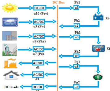
In this section, we present a smart micro-grid that consists of: two storage elements (batteries), three sinks (loads) and one virtual sink (external grid connection), one node (DC Bus), four sources (PV, Wind, Hydroelectric, and Diesel generators), and one virtual source (external grid connection). A grid connection is a sink when it is buying energy, and a source when selling energy. The block diagram of the smart micro-grid is shown in Fig 1.
B. Control-oriented Model
Since all the components (excluding sinks) are connected to a single node (DC Bus) through flow handling elements, they are all considered as manipulated inputs. The states of the smart grid are defined to be the state of charge of the storage elements.
State variables:
xband xhare the state of charge of the batteries (lead-acid and
hydrogen respectively): x(k)
[xb(k), xh(k)]TFig 1. Block diagram of the smart micro-grid
Control input variables:
u(k)
[Pb1(k), Pb2(k), Ph1(k),Ph2(k), Pg1(k),Pg2(k), Pd(k),Phy(k), Pw(k), Ppv(k)]T
where Pb1and Pb2are charged power and discharged power of
the lead-acid battery; Ph1 and Ph2 are the charged and
discharged power of the hydrogen battery; Pg1and Pg2are the
exported and imported power into/from the external grid; Pd,
Phy, Ppv, and Pw stand for the power supplied to the DC Bus by
the diesel, hydroelectric, wind, and photovoltaic generators respectively;
Disturbance variables:
d1 is the industrial load, d2 is the residential load, and d3 is the
DC-load. The disturbance vector d consists of the three loads.
d(k)
[d1(k), d2(k), d3(k)]TThe matrices and vectors that define the system and its constraints are given as follows:
1 0 0 1 0 0 0 0 0 0 0 0 0 0 0 0 0 0 0 0 1 1 1 1 1 1 bc bd hc hd p η η η η = − = − − − − = − − − A B B where:
ηhc and ηhd are the charging efficiency and discharging
and ηbc and ηbd are the charging efficiency and discharging
efficiency of the lead-acid battery respectively.
xmin = [0 0]T , xmax= [100 100]T
umin (k)= [0 0 0 0 0 0 0 0 0 0]T,
umax(k)= [35 10 35 18 18 18 18 18 Pp
w(k) Pppv(k)]T Kw
where Ppw(k) ≤ 18Kw and Pppv(k) ≤ 18kW are the energy
generation profiles of the wind and photovoltaic generators respectively.
The equilibrium equation of the DC Bus according to (2) is given by:
Eu= [-η1η2 -η3 η4 -η5 η6 η7 η8 η9 η10] , Ed= [-1 -1 -1]
where ηi, i=1,…,10 are the electrical performance indeces of
associated power sources/sinks that consider transmission and control units losses.
α1
[α1pb1, α1pb2, α1h1, α1h2, α1g1, α1g2, α1d, α1hy, α1w, α1pv]Twhere:α1pb1, α1pb2, α1h1, α1h2, α1g1, α1g2, α1d, α1hy, α1w, α1pv are
fixed costs corresponding to the control input variables respectively. Their values are shown in Table 1.
MPC objective function’s matrices and parameters
b b h h g g d hy w pv c 1 0 0 1 diag(c ,c ,c ,c ,c ,c ,c ,c ,c ,c ) . = = = x Q R S W Q
where: cb, ch, cg, cd cd, cpv, cw andchy are positive weight
coefficients (≤ 1) for the lead-acid battery, hydrogen battery, grid connection, diesel, solar, wind, and hydroelectric generators respectively. Their values are shown in Table 1.
Wcis a scalar weighting factor for the terminal state.
We have considered days with bad weather conditions, whereby all the generators are required to be in operation, in order to satisfy the load demands. If they cannot satisfy the demand, then the batteries, the external grid, and the diesel generator will compensate the shortage one after the other. Initial values of the subsystems, as well as the state of charge of the batteries are set to zero. The simulations were made for 96 hours (4 days).
The diesel generator (1-1.3 kWh) was operated in summer during the first six hours of the day, and in winter in the afternoon for six hours. It was supplying 1.3 kWh in the first hour and 1 kWh in the remaining hours.
The batteries were used during the first two hours of the day. They were delivering 2 kWh in the first hour and 1 kWh in the second hour.
1 kWh was bought from the external grid during the second hour of the day.
All the plots in this study have been made using Tomlab (CPLEX) and YALMIP (IBM CPLEX) in Matlab environment.
System parameters Control parameters Parameters Values in Parameters Values
kW Pmaxpv 18 Np 24 Pmaxw 18 Nc 24 Pmaxhy 18 cpv 0.2 Pmaxd 18 cw 0.3 Pmaxb1 35 chy 0.4 Pmax b2 18 cb 0.75 Pmax h1 35 ch 0.75 Pmaxh2 18 cd 1 Pmaxg1 18 cg 0.75 Pmaxg2 18 Q as defined previously ηbc 0.95 R as defined previously ηbd 1 α2 0.0 ηhc 0.85 α1pb1= α1pb2= α1h1= α1h2 2.2 ηhd 1.0 α1g1=α1g2 3.0 ηi i=1,…,10 1.0 α1d α1hy=α1w α1pv ρ 3.3 2.1 2.0 1.0 δ (35 35)T
Table 1. System and control parameters’ values
The prioritization weights: λ1=25; λ2= 12; λ3=0.1. The higher a coefficient is, the stronger is the penalization of its corresponding subsystem.
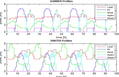
Fig 2 shows data of expected energy flow from the generators as well as the load demand for a single weekday. These data constitute the profiles i.e. forecast of energy generation and load demands used for computing reference set-points for the MPC tracking.
Fig. 2. Available maximum power in the sources and load demands
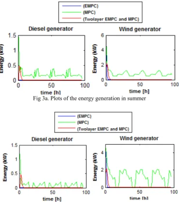
The profile of a generator represents the maximum power that can be ideally produced by the generator. Figures 3a and 3b show a sample comparison of the energy production of the diesel and wind generators in summer and winter respectively.
Fig 3a. Plots of the energy generation in summer
Fig 3b. Plots of the energy generation in winter
Remarks:
As it can be seen form Figures 3a and 3b), the standard Economic MPC strategy outperforms the other strategies, since it yields the lowest energy production.
The main goal of this study is to minimize the costs of energy production. Energy from the diesel generator is more expensive than from renewable energy sources. Figure 3a and 3b show that the EMPC strategy has minimized the most the operation of the diesel generator.
This work shows also that, one-layer approach is economically superior to a hierarchical two-layer scheme. Similar result was obtained in [8], [13].
Finally, it can be seen (Table 2) that, the EMPC produces the lowest daily economic costs, thereby proving its superiority to the other strategies. Table 2 presents a comparison of the three MPC approaches' daily economic costs.
Economic MPC EMPC + MPC tracking (two-layer) MPC tracking Summer economic cost 651.3373 699.0715 719.3985 Winter economic cost 724.3611 772.0917 814.4630
Table 2. Quantitative comparison of the economic costs
V.
Conclusions
This paper has proposed the application of Economic Model Predictive Control (EMPC) to control a grid connected smart micro-grid consisting of several subsystems namely some photovoltaic (PV) panels, a wind generator, a hydroelectric generator, a diesel generator, and some storage devices
(batteries).
We have first introduced the standard Economic MPC. Then for comparison, the standard tracking MPC, and finally a hierarchical two-layer MPC consisting of the integration of both. Comparing the daily economic costs of the subsystems in the proposed case study, it has been shown that economic MPC yields the best economic result, because the energy consumption is the lowest. The result of this study shows that, EMPC strategy can be successfully used to control energy dispatch in smart micro-grids.
The next tasks for completing this study will be devoted to tackling additive disturbances, stability issues, and optimizing the selection of the controllers' weights using robust optimization methods and machine learning techniques.
Acknowledgments
This work was supported by Spanish Government (MINISTERIO ECNONOMIA Y COMPETITIVIDAD) and FEDER under project DPI2014-58104-R (HARCRICS).
References
[1] J.M. Maciejowski, Predictive Control with Constraints, Prentice Hall, New Jersey, 2002.
[2] W. Liuping, Model Predictive Control System Design and
Implementation Using MATLAB, ISBN 978-1-84882-330-3, 2009. [3] Halvgaard, R., “Model Predictive Control for Smart Energy Systems“,
PhD thesis, DTU Denmark, 2014.
[4] I. Prodan, and E. Zio, “A model predictive control framework for reliable microgrid energy management”, International Journal of Electrical Power & Energy Systems, vol. 61, pp 399–409. 2014. [5] M. Pereira, D. Limon, T. Alamo, and L. Valverde, “Application of
Periodic Economic MPC to a Grid-Connected Micro-grid”, 5th IFAC Nonlinear Model Predictive Control Conference International Federation of Automatic control, Sevilla, Spain, 2015.
[6] D. Bica, C. Dumitru, A. Gligot, and A. Duka, “Isolated hybrid solar-wind-hydro renewable energy systems”, Renewable Energy, T J Hammons (Ed.), InTech, pp. 821–826. 2009.
[7] P. Tatjewski, “Advanced control and on-line process optimization in multilayer structures”. Annual Reviews in Control, vol. 32(1), pp. 71 – 85, 2008.
[8] J.M. Grosso, “On Model Predictive Control for Economic and Robust Operation of Generalised Flow-based Networks”, PhD thesis, UPC, Barcelona. 2014.
[9] J.B. Rawlings, D. Angeli, and C.N. Bates, “Fundamentals of economic model predictive control”. In Proc. 51st IEEE Conference on Decision and Control (CDC), pp. 3851–3861. 2012.
[10] M. Ellis, and P.D. Christofides, “Integrating dynamic economic optimization and model predictive control for optimal operation of nonlinear process systems”. Control Engineering Practice, vol 22(0) pp. 242–251. 2014.
[11] J. A. Rossiter, Model-Based Predictive Control: A Practical Approach, CRC Press, Boca Raton, FL. 2003.
[12] W. Liu, J. Qi, X. Chen, and P. H. Christofides, “Supervisory Predictive Control of an Integrated Wind/Solar Energy Generation and Water Desalination System” In Proceedings of the 9th International Symposium on Dynamics and Control of Process Systems, Leuven, Belgium. 2010.
[13] M. Nassourou, V. Puig and J. Blesa. Robust optimization based energy dispatch in smart grids considering demand uncertainty, 13th European Workshop on Advanced Control and Diagnosis, 2016, Lille, Vol 783 of Journal of Physics: Conference Series, pp. 012033, 2017.