- First Empirical Results -

Genetic-Based Trading Rules

-

A New Tool to Beat the Market With?

-

First Empirical Results

-

Andreas Frick’), Ralf Herrmann’), Martin Kreidler”, Alexander Narr” and Detlef Seese‘)

Abstract

We investigate price-based heuristic trading rules for buying and selling shares. This is accompanied by transforming the time series

of

share prices using Point & Figure (P&F) Chart Analysis. On the basis of the binary representation of those charts we used a genetic-based Machine Learning System to generate trading strategies by the classification of different price formations. We used two different evaluation methods: 1) comparing the return

of

any considered trading strategy with the corresponding riskless interest rate and the average stock market return, and

2)

using its risk-adjusted expected return as a benchmark instead of the average stock market return. The latter is calculated using the Capital Asset Pricing Model (CAPM). The resulting binary example data is iteratively processed by our learning system. We used

as

input data

1.120.278

intraday stock prices from the Frankfurt Stock Exchange (FSE). We show to which degree of correctness different price formations ca be classified by our system and how such rules look like.

R&Um6

Nous ktudions des prix-bash rkgles de commerce pour acheter et vendre des actions. Nous ferons cela en transformant la drie des prix d’actions en utilisant point & figure chart analyse. De

ces

dernikres, nous reqwrons des formations, dont nous pouvons c r k r des rkgles pour la classification par notre gknktique mkhanique systkme d ’apprentissage. Nous ferons 1 ’evaluation des formations en deux mkthodes: L’un, par comparer les taux de rendement de chaque stratkgie de commerce avec l’int6ret sans risque et le moyen taux de rendement de la bourse,

1

’autre par comparation avec le risque-adapt6 taux de rendement calculk avec le capital asset price model (CAPM).

Les

donnks d ’exemple

sont

process& avec notre systkme d ’apprentissage. Nous avons utilid

1.120.278

entre-jour prix d’actions du Frankfurt Stock Exchange (FSE). Nous montrons l’exactitude de la classification des prix formations diffkrents et les rkgles correspondants avec ceux.

Keywords

Technical stock market analysis, point

&

figure charts, trading rules, machine

learning, genetic algorithms.

Acknowledgement:

We want

to

thank

Costanza

Torricelli, Hermann Giippl and

David Robbins Griswold

for helpful comments and suggestions. Usual caveat

applies.

')

_{Institute for Decision Theory and Enterprise Research, University of Karlsruhe, D - 76128}

Karlsruhe (Germany); Tel:

+

49-721-608 6037, Fax:

+

49-721-693 717, E-mail: herrmann~~.wiwi.uni-karlsruhe.de, {afr

I

kmr

1

ana

I

seese}@aifb.uni-karlsruhe.de

Institute for Applied Computer Science and Formal Description Methods, University of Karlsruhe, D

-

76128 Karlsruhe (Germany).

1

Introduction

1.1

General Considerations

In the last few years, Genetic Algorithms proved to be a useful tool for computing approximative solutions of hard problems (especially problems for which no general efficient solution is known or those which are provably hard, e.g. NP-hard problems). One such hard problem is forecasting in stock markets. By forecasting, we mean finding rules’ that tell an investor when to buy a particular share and when to sell it. On the one hand, in our classification system the considered buy and sell rules result from the actual return.of the share and the movements of the stock market in the past, on the other hand they result from the expected return of the share and the expected return of the whole stock market in the future.

Our objective is to show how such a system can be applied to share prices in order to generate trading strategies and to investigate the obtained trading rules.

1.2

Genetic-Based Machine Learning

One of the most challenging topics in the Artificial Intelligence research area is Ma- chine Learning. The aim is to construct new or to improve already acquired know- ledge by using input information. The most active area [MiKo] has been Symbolic Empirical Learning, the creation or modification of general symbolic descriptions, whose structure is a-priori unknown. Such symbolic descriptions frequently have to be developed from a set of given concept examples [Lan, MiKo], because in many practical domains it is very easy to come up with concepts.

Holland [HoRe] introduced the idea of using Genetic Algorithms to improve rules already given or generated newly from scratch. His approach to such a classifier system, well-known as the “Michigan Approach”, works by manipulating a set (or a population) of rules that have the shape of Horn formulas. If the aim is to improve a given set of rules, then the initial rule population equals the given rule set, otherwise

attribute

position of the engine

an initial rule set is created at random. This population of rules is then tested against the set of examples by Supervised Learning. Rules that classify wrongly are punished and rules that classify correctly are rewarded, such that each rule gets a fitness value according to its classification correctness. Most implemented systems have more complicated mechanisms to distribute the reward and they also transfer reward from the bad to the good rules.

It

is also possible to extend this mechanism by enabling reward transfer along calling queues such that a system can learn multistep tasks. The rules are regularly processed by a Genetic Algorithm in order to remove the bad rules and improve the good ones, i.e. the rules are selected by a probability according to their fitness and recombined by the two “genetic” operations Crossover and Mutation. The main idea is to improve the already good rules by enforcing an interchange of rule components and by trying out new, untested rule elements. Bad rules have little chance of survival and of becoming incorporated into the next generation’s rule set.

value

front, center, rear

Below, a simple example is given to show what such rules look like. The brand of automobiles shall be identified depending on five properties. The attributes (by their sequence) and their domains are:

number of cylinders drive

4, 5 , 6, 8 , 12

front, rear

I

position of the gearbox

11

front, center, rear

I

type Porsche:

attributes

rear engine and rear gearbox and six cylinders or front engine and rear gearbox and eight cylinders

I

Mercedes:

11

front engine and front gearbox and engine along

I

vw:

I

Audi:

11

front engine and front gearbox and engine traverse

I

rear engine and rear gearbox and four cylinders

All concepts belonging to a class form its positive example set; all other concepts form its negative example set. Hence, a concept C is a disjunction of expressions c1.

.

.c, :

( C I V

...

v c , )

*

c,

with the ci being conjunctions of single selectors of the form (attribute, relation, value), e.g. (e = f ) stands for “engine in front”. The above example concepts can now be formalized as follows2:

( ( e = r ) A ( g = r ) A ( c = 6 ) ) V ( ( e = f ) A ( g = r ) h ( c = 8 ) ) I

P

- M

- A

= + v

( ( e =

f )

A (9 =

f )

A ( 0 =

4 )

( ( e =

f )

A (9 =

f )

A ( 0 =

4 )

( ( e = r ) A (g = r ) A (c = 4 ) )

Furthermore, rules like the first one now can be split into two separate rules:

( ( e = T ) A (g = r ) A (c = 6 ) )

*

P

( ( e =

f )

A (g = r ) A (c = 8 ) )

*

P

Rules of this format are called Horn Formulas and are the foundation of resolution techniques e.g. used in

PROLOG,

a logic-based high-level programming language. Now, the main problem is to construct rules from an example set in such a way that every example is covered by a rule, but none of the examples are classified into a wrong class. One of the possible methods is to use a genetic-based classifier system.

Additionally, crossover and mutation also should be explained a little more closely. It is assumed that the following two rules have been selected for reproduction due to

their superior classification capabilities:

( ( e =

f )

A (g = f ) A (0 =

t )

A ( c = *) A ( d =

* ) )

===?- A

( ( e = r ) A ( g = r ) A ( 0 = *) A ( c = 4) A ( d =

*))

===3 V

T h e

‘‘*”

symbol denotes an attribute that is relaxed, i.e. the attribute value does not affect the classification. Now, a crossover after the third attribute results in the following two new rules:

( ( e = f ) A (g = f ) A (0 =

t )

A ( c = 4) A ( d =

*))

==+

V

and

( ( e = r ) A ( g = r ) A (0 = *) A ( c =

*)

A ( d =

*)) ==+

A

The mutation operator now changes single attribute values in their corresponding domain, e.g. the second attribute of the first rule and the last attribute of the second rule. This results in the following two new rules:

( ( e =

f)

A ( g = r ) A (0 = t ) A ( c =

4)

A ( d =

*I)

==+

v

and

( ( e = r ) A ( g = r ) A (0 = *) A ( c =

*)

A ( d = r ) ) ==+ A

A very serious problem of using a classifier system is the transformation of the given example data in a format the system can process. In almost every case information is lost during this step. Thus, finding the right way of transformation is essential for obtaining good classification results. For our transformation process, we have chosen the methods of Point & Figure Technique which we introduce below:

1.3

The Point

&

Figure Technique

T h e essential problem a n investor in a stock market is confronted with is the exact timing of his transactions - when to buy and when to sell shares, - presumably

the deciding factor of success or failure. The Point & Figure (P&F) technique is a

heuristic method that supports his decision making by giving buy and sell signals. This kind of Chart Analysis restricts to just one aspect of market activity - price

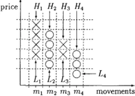
change and its reversals. Time factors (i.e. length of the price-trends) or volume data are not taken into consideration. Hence, a P & F Chart has no horizontal time scale and looks like a series of vertical “X”s and “O”S, placed into columns from left to right. Each “X” and “0” fills a box which represents the minimum relative price movement with significance for the analysis. Figure 1 illustrates the procedure. The boxes are visualized by dashed lines. Due to its heuristic character, there exist

Figure 1: Point & Figure Chart

different procedures for creating such a chart (e.g. [Bau, Eng, Hoc, Mur, TO], Well). We used the following one:

“X”

signs in the column stand for an increase while

“0” signs stand for decreasing share prices. Such price movements are entered continuously into the chart. Whenever a reversal in the price movement occurs, the sign representing the new price movement is written into a new column. Therefore, each column consists of only one kind of sign. For the practical application of this method, two decisions have to be made a-priori: First we have to decide which box size is appropriate and second we have to define the reversal criteria. The box size is influenced by the time frame and the volatility of the observed market. In our study we follow a suggestion of Welcker [Well for German stocks (standard conversion). Values for his approximation can be found below:

share price

10

-

14 0.2

14 - 29 0.5

price change

/

box

29 - 60 1

60 - 100 2

share price

100 - 140

price change

/

box

140 - 290 290 - 600

600 - 1000 20

F

l

Based on this chart, the P&F Analysis tries to identify buy and sell signals, e.g. penetrations of support/resistance lines.

2

How to learn from Stock Market Data

2.1

Conversion of the Stock Market Data

For the efficient application of the classification system, it was necessary to convert the P&F Charts and trading rules into an appropriate binary representation. We accomplished this within two steps, which are explained below:

1. During the first step, the stock prices are converted into the

P&F

Charts. Each price movement m ; (each column in the P&F Chart) is represented by its highest ( H i ) and its lowest

( L ; )

value. An illustration is given in Figure 1.

The first entry specifies the direction of the first movement in the chart. “0”

stands for a downward and “1” for an upward move. The other entries contain the highs and lows of the following price movements. Because after an upward movement always follows a downward movement and vice versa, it is sufficient to define the direction of the first movement to determine the direction of all movements in the chart (see Figure 1).

2. In the second step we have to transform the above representation into a new form which allows us to generate buy and sell rules based on

P&F

Chart Analysis. The trading rules of the P&F Technique are mainly based on com- parisons of both the highs and the lows of the different price movements of the formation under consideration.

A

typical example of such a trading rule is: Buy a share if the top of the following “up” is higher than the top of the preceding “up” and the bottom of the following “down” is higher than that of the preceding “down”. Thus, the data was transformed into the following format:

(011)

,

2

,

2

,

3

H 3 H4 H4

H i

’ X ’ z ’ Z

The comparisons of the tops and those of the bottoms of the considered move- ments are conducted by calculating the quotients

$

and

$

with

i

#

j. These quotients describe the price pattern for our classification system completely. If the top of movement

(i

+

1) is higher than the top of movement

i,

then

>

1. This is analogous for the lows. The sketched trading rule above is formalized in the following manner (using the notions of propositional logic calculus with its standard semantics):

> H;

and thus,

A

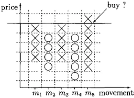
similar sell rule for example is: Sell a share if the bottom of the follow- ing “down” is below the bottom of the preceding “down” and the top of the following “up” is below that of the preceding “up”. More formally:

By this kind of representation it is also possible to express resistance and sup- port lines. For example, the penetration of a resistance line can be formalized as

[

(2

= 1) A

(2

>

I ) ]

+

Buy, and is visualized in Figure 2.

Figure 2: Resistance Line

Note that up to now we have only got formation patterns, but no decision signals (i.e. buy or sell), since we have only showed how the stock market data was converted using the P&F Technique and that it is possible with our representation to formalize conventional technical trading rules. We now explain how the above obtained form- ations are evaluated (i.e. provided with a decision signal) and how the classification process afterwards works.

To initialize our rulebase the first population of rules is created at random. T h e patterns obtained now have to be evaluated and classified. We do this in the following way: According to a given time interval (30 days, 90 days, 6 months, 1 year) which can be chosen by the user of our system, beginning for each example a t the last price of the considered price formation, the return of the recommended trading decision for the considered time interval is looked up in the database in order to decide whether the formation was a profitable buy or sell signal. This is accomplished by comparing the return of the particular trading strategy with the riskless interest rate and either the market return or the expected riskadjusted return for the considered time interval.

The expected riskadjusted return is calculated using the Capital

Asset

Pricing Model (CAPM) [Sha]. The CAPM postulates the following relation between risk and return of a risky asset:

Hereby, E ( r j ) is the expected return of asset

i,

rf denotes the riskless interest rate,

E ( ~ M )

is the expected return of the market portfolio,

V A R ( T M )

the variance of the market return and C o V ( r ; , r ~ ) is the covariance between the returns of the risky asset

i

and the market portfolio

M .

(E(r,) - r j ) is the “Riskpremium” paid for

the risk of asset

i

measured by

pi.

We treat the resulting trading strategies as a risky asset that is valuable using the CAPM. The classification of the formations into buy and sell signals is now quite straightforward: If the return of a share is higher than the corresponding market return resp. its expected riskadjusted return and it is higher than the riskless rate then it is a buy signal. Otherwise it is a sell signal.

Hence, we have obtained trading decision examples that can be further processed by a learning system. We used our modified version of Goldberg’s MSCS to extract rules from this data. The system’s rule set is continuously tested against the example

set and the amount of correct classifications is reported. From the textual output then figures are created showing the progress of the classification process.

3

Results

3.1

Technical Details

In our approach we used

MSCS,

a system based on the ANSI-C-version [Hei] of the Simple Classifier System proposed by Goldberg [Gol], which we have slightly modified and improved to enhance its stability [Fri]. We ran our system on a Sparc Station. The example data produced by the conversions described above has been divided into two parts: a training sample to learn from and a test sample to evaluate the rules extracted from the training sample.

3.2

Datasample

We ran our system with 1.120.278 intraday prices of the Frankfurt Stock Exchange from the time interval between January 11, 1989 and May 30, 1994. Our sample contains all 30 shares of the Deutscher Aktienindex (DAX). The riskless interest rates used in our study are the Frankfurt Interbank Offer Rates (FIBOR). To calculate the market return, the DAX was used as a proxy. All prices were adjusted for dividend payments and capital adjustments and were provided by the Karlsruher Kapitalmarktdatenbank (KKMDB) [Her].

3.3

The Classification

Since only few datasets could be extracted from 3- and 5-point Reversal Charts, we implemented a modified first step of the conversion which takes a percentage as

an input which is the minimal percentage that triggers a trend reversal of a share (compare section 2.1 first step). This allows us to extract more formations (in our

runs we used 2 percent which roughly corresponds to half a box) on the one hand, on the other hand, the resulting charts are not so general any more.

The modified conversion can be looked at as special version of charts whereby the trigger to start a trend reversal can be fine-tuned continuously, while the 1-, 3- and 5-point Reversal Charts are discrete. The conversion with 1-Point Reversal Charts and the modified conversion proved to be good means for our purposes.

Using the

MSCS,

we tried to find signals for gainful buy and sell strategies on the stock market. We ran the

MSCS

for 100,000 generations with the standard and the modified conversion. The main problem then was to tune in the parameters both of the conversion and of the MSCS in such a way that the MSCS converged.

Not only the minimal value for a trend reversal is a critical parameter, but also the number of movements per rule. The more moves ordered to a rule, the less training examples can be found for that particular rule. Furthermore, too few rules can be found, if too many movements are collected within a rule. It is a natural conjecture that too many movements per rule made the formations too complex. Our tests confirmed this, since then the MSCS could not generate a rule set with sufficient quality any more.

We ran our tests mainly based upon the following 4 settings:

1. whole

DAX

sample within a 90 day time interval, 3 movements per rule and

(a) Welcker approximation using 1 Point Reversal Charts, (b) modified conversion with 2 percent reversal criteria;

2. single stocks within a 90 day time interval, 3 movements per rule and

(a) Welcker approximation using 1 Point Reversal Charts,

(b) modified conversion with 2 percent reversal criteria.

We used in the classification process for all four diagrams the market return and the riskless interest as benchmarks. The diagrams show the percentage of correctly

identified trading signals while learning from the training dataset. After finishing the learning process the resulting rules are tested by using them to classify the test dataset.

In our tests the rulebases obtained are able to detect trading signals with an average correctness of over 60 percent in the training dataset. It is important to know that this is only an average value, i.e. there are rules in the final rule base that give even better results. The application of the rulebases obtained on the test datasets yields similiar results (compare Figure 4).

Figure 3 shows four of our results: The two diagrams on the left correspond to l . ( a ) (above) and l.(b) (below), the two diagrams on the right-hand side correspond to 2.(a) (above) and 2.(b) (below). As input data we used stock prices of Volkswagen. T h e 5 axis gives the number of generations, the y axis denotes the percentage of

correct classified examples.

It is obvious that both diagrams below have higher percentage of correct classifying trading rules; this is due to the modified conversion which can be more easily fine- tuned. We observed that generally the modified conversion brought slightly better results. The application of the final rulebase on the test data (example (2.(b)), diagram right below) results in the evalution protocol shown in Figure 4.

39 Regeln m i t 163 Termen

Jedes Objekt i m S c h n i t t durch 0 Objekte n i c h t k l a s s i f i z i e r t

0 Objekte f a l s c h und korrekt k l a s s i f i z i e r t

43 Objekte f a l s c h k l a s s i f i z i e r t 60 Objekte korrekt k l a s s i f i z i e r t

1.0097 Regel(n) k l a s s i f i z i e r t

Figure 4:

A

resulting

MSCS

evaluation protocol

The final rulebase consists of 39 rules that have all in all 163 attributes (mainly comparisons of highs and lows). On average, each test formation is classified by

1.0097 rules. Zero examples are not classified, zero examples are correctly and wrongly classified, i.e. there is no example such that two rules match that example but give different trading signals (at least one rule is a buy rule and one rule is a sell rule). 43 examples are wrongly classified while 60 rules are correctly classified by the rulebase.

3.4

Example:

A Generated Trading Rule

Below, we show one trading rule obtained by the classification process of the

MSCS

after 100.000 generations using the time series of Volkswagen share prices and clas- sical conversion (2.(a)):

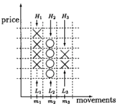
This has the following meanings: We built our trading rules based upon three move- ments, i.e. there are three highs and three lows which can be compared with each other, respectively. We refer to them as H17 H2, H3 and L1, L2, L3. The resulting values are divided into 6 intervals3:

1 2 3 4

5

6

The above trading rule can be explained more clearly as follows:

[(first move upward) A

(2

E 4) A

(2

E 4) A

(2

E 311

+

BUY Figure 5 visualizes the price formation:

PI

Figure 5: The P&F formation corresponding to the buy rule of our example

Note that in the rule any information about L1 is dropped out due to wildcards. We visualize this in figure 5 by the three dots in the leftmost formation. The complete rulebase for this particular example is given in the appendix A.

4

Summary and Ongoing

Work

We investigated heuristic trading rules based on Point & Figure Chart Analysis. The results obtained allow to identify rulebases which are able to detect trading

signals with an average correctness of over 60 percent. Until now we investigated only the correctness of the classification process, for the future we have to focus on the performance of the resulting trading strategies.

There are two main directions of ongoing research: First, a lot of modifications on the “technical” side can be done: The implementation of variable formation length and the incorporation of the box size into the classification process offers new interesting fields of research. Furthermore, it is interesting to implement the “Pitt’s Approach” for the

MSCS

in order to compare results to that of the “Michigan Approach”. An- other interesting topic is the performance of the obtained rules: Unfortunately, up to now, we are unable to produce the fitness values which correspond directly to the performance of the rules. Implementing an additional module that logs this values to check and evaluate them statistically should give new interesting insights about the performance of every single trading rule. This motivates the idea of using al- ternative rewarding functions: Instead of just investigating whether a rule based trading strategy performs better than the market or the riskless interest, it would be interesting to consider how much better such obtained trading rules are.

A

straight- forward rewarding function would be the accumulated return or the accumulated excess return of the trading rules.

Besides this, we think that a “filter” routine should be implemented that checks any rule which is generated by the Genetic Algorithm if its structure is consistent with a

P&F

Chart formation (compare appendix A). Indeed, rules not consistent with such formations have only very limited chances to survive (since they never participate the auction and hence do not obtain a reward which strengthens their fitness), but in any case, they “waste” the rulebase. The results using such a filter routine are inasmuch of particular interest, since this would answer the question, if such rules are necessary for the Genetic Algorithm to find good classification rules. The former guarantee that the Genetic Algorithm can theoretically search within the complete solution space; if the above rules are removed from the current population, it is possible that there are parts of the solution space which are not longer reachable any more.

A

further idea is to initialize the

MSCS

with traditional

P&F

trading rules4.

It is interesting to investigate if the system is able to improve such traditional trading rules and up to which degree.

The second direction of ongoing work is on the “application” side: An interesting topic is the selection of the stocks. Up to now, we have only treated either single stocks or the whole DAX sample. It would be interesting to consider particular groups of stocks: Stocks of the same industry group (e.g. automobile stocks) or stocks that are highly correlated. Especially, it should be very interesting to apply our system to larger datasamples like price data of the Deutsche Termin Borse (DTB) for derivative securities. Then we would be able to apply the full “power” of our system.

Furthermore, the application of the system should allow us to examine if there exist price formations in the stock markets or derivative markets that give reliable buy and sell signals and whether it is possible to construct an adaptive system based on Genetic Algorithms to generate new trading strategies with which it is possible to beat the market with.

A One

Example Rulebase

Below, we present the complete rulebase for example 2.(a) of subsection 3.4. It is obvious that the rules have different length,that means some rules are more special while others are more general. Furthermore, it is important to notice that due to the “genetic” way of building new rules from old ones, it is possible that rules can be generated that are not applicable (since in their condition part matches only formations that cannot exist due to the prescriptions of the P&F Chart Technique).

I F h-1-rel-2 = 4 6 1-1-rel-2 = 3 & 1-1-rel-3 = 4 & h-2-re1-3 = 4

I F F l a g = 1 & h-1-rel-2 = 4 & 1-1-rel-2 = 3 & h-1-rel-3 = 4 6 1-1-rel-3 = 4

I F F l a g = 0 & h-1-rel-2 = 4 & 1-1-rel-2 = 3

& 1-1-rel-3 = 4 & h-2-re1-3 = 3

I F F l a g = 1 & h-1-rel-2 = 4 & 1-1-rel-2 = 3

& h-1-rel-3 = 3 & 1-1-rel-3 = 4

=> S i g n a l = BUY => S i g n a l = SELL

& 1-2-re1-3 = 3 => S i n n a l = SELL

I F 1-1-rel-3 = 3 => S i g n a l =

BUY

I F F l a g = 1 & 1-1-rel-3 = 4 & h-2-re1-3 = 4

I F 1-1Ireli3 = 4 => S i g n a l =

BUY

I F 1-1-rel-2 = 3 & 1-1-rel-3 = 4

& h-2-re1-3 = 3 => S i g n a l =

BUY

I F F l a g = 1 & h-1-rel-2 = 4 & h-2-re1-3 = 4

& 1-2-re1-3 = 3 => S i g n a l =

BUY

I F h-1-rel-2 = 4 & 1-1-rel-2 = 3

& 1-1-rel-3 = 4 => S i g n a l =

BUY

I F F l a g = 1 & h-1-rel-2 = 4 & 1-1-rel-2 = 3

& h-2-re1-3 = 4 & 1-2-re1-3 = 3 => S i g n a l = SELL I F h-1-rel-2 = 4 & 1-1-rel-2 = 3

& h-2-re1-3 = 3 => S i g n a l =

BUY

I F Flag = 1 & h-1-rel-2 = 4 & 1-1-rel-2 = 3

& h-1-rel-3 = 4 & 1-1-rel-3 = 4

& h-2-re1-3 = 3 => S i g n a l = SELL

I F h-1-rel-2 = 4 & 1-1-rel-3 = 4

& h-2-re1-3 = 4 & 1-2-re1-3 = 3 => S i g n a l =

BUY

I F h-1-rel-2 = 4 & 1-1-rel-2 = 3

& h-2-re1-3 = 4 & 1-2-re1-3 = 3 => S i g n a l =

BUY

I F h-1-rel-2 = 4 & 1-1-rel-2 = 3

& 1-1-rel-3 = 4 & h-2-re1-3 = 4

& 1-2-re1-3 = 3 => S i g n a l =

BUY

I F 1-1-rel-2 = 3 & 1-1-rel-3 = 4

& h-2-re1-3 = 4 & 1-2-re1-3 = 3 => S i g n a l =

BUY

I F F l a g = 1 & h-1-rel-2 = 4 & h-2-re1-3 = 4 => S i g n a l = SELL I F h-1-rel-2 = 4 & 1-1-rel-3 = 4

& h-2-re1-3 = 4 => S i g n a l =

BUY

I F 1-1-rel-3 = 4 & h-2-re1-3 = 4

& 1-2-re1-3 = 3 => S i g n a l =

BUY

I F F l a g = 1 & h-1-rel-2 = 4 => S i g n a l =

BUY

I F F l a g = 0 & h-1-rel-2 = 4 & 1-1-rel-2 = 3 => S i g n a l =

BUY

I F F l a g = 0 & h-1-rel-2 = 4 & 1-1-rel-2 = 3

& h-2-re1-3 = 4 & 1-2-re1-3 = 3 => S i g n a l =

BUY

I F h-1-rel-2 = 4 & 1-1-rel-2 = 3

& 1-1-rel-3 = 3 => S i g n a l =

BUY

I F F l a g = 0 & h-1-rel-2 = 4 & 1-1-rel-2 = 3

& h-1-rel-3 = 3 & h-2-re1-3 = 4

& 1-2-re1-3 = 3 => S i g n a l =

BUY

I F Flag = 1 & 1-1-rel-2 = 3 & 1-1-rel-3 = 4

& h-2-re1-3 = 3 => S i g n a l =

BUY

I F h-1-rel-2 = 4 & 1-1-rel-2 = 3

& 1-1-rel-3 = 4 & h-2-re1-3 = 3 => S i g n a l =

BUY

I F F l a g = 1 & h-1-rel-2 = 4 & 1-1-rel-2 = 3

& h-2-re1-3 = 4 => S i g n a l = SELL I F F l a g = 1 & h-1-rel-2 = 4 6 1-1-rel-2 = 3

& 1-1-rel-3 = 4 & h-2-re1-3 = 3 => S i g n a l = SELL I F

I F

-

111Irel12 = 3 & hI2Ire113 = 4

=> S i g n a l =

BUY

h-1-rel-2 = 4 6 1-1-rel-2 = 3 => S i a n a l =

BUY

& 1-2-re1-3 = 3

-

I F hIlIrelI2 = 4 & 1Il-relI2 = 3

& h-1-rel-3 = 4 & h-2-re1-3 = 4

I F h-1-rel-2 = 4 & 1-1-rel-2 = 3

& h-2-re1-3 = 4

I F F l a g = 1 & h-1-rel-2 = 4 & 1-1-rel-3 = 4

# 34 rules w i t h 127 terms

=> S i g n a l =

BUY

=> S i g n a l =

BUY

=> S i g n a l = SELL

Endnotes

‘We note that the term ‘‘rule’’ is used in two different meanings in Technical Chart Analysis and Machine Learning.

2The application of Genetic Algorithms was originally applied on capital market data by Bauer [Bau] and Allen/Karjalainen [AIKa]. In contrast to our work, they do not make use

of the P&F Chart Technique.

3Since share prices are always positive all calculated quotients are positive. The number of intervals is also a n input parameter to our system.

4Up to now, the first generation of the population in the Genetic Algorithm is created at random.

,

References

[AIKa] F. Allen and

R.

Karjalainen, “Using Genetic Algorithms To Find Tech- nical Trading Rules”, Technical Report, Wharton School of the University of

Pennsylvania, Rodnely

L.

White Center for Financial Research, May 20, 1995. [Bau]

R. J.

Bauer Jr., “Genetic Algorithms and Investment Strategies”,

J.

Wiley &

Sons, Inc., New York, 1994.

[Eng] W.

F.

Eng, “The Technical Analysis of Stocks, Options & Futures - Advanced Trading Systems and Techniques”, Probus Publishing, Chicago, Ill., 1988. [Fall

E. G.

Fama, “Efficient Capital Markets:

A

Review of Theory and Empirical

Work”, Journal of Finance, May 1970, pp. 383-417.

[Fa21

E. G.

Fama, “Foundations of Finance”, Basic Books, New York, 1976.

[Fri]

A.

Frick, “Erweiterungen des Goldbergschen ‘Simple Classifier System”’, Dip- lomarbeit, Institut

AIFB,

Universitat Karlsruhe, 1995.

[FHKNS] A. Frick, R. Herrmann, M. Kreidler, A. Narr and D. Seese, “A Genetic- Based Approach for the Derivation of Trading Strategies on the German Stock Market”, to appear in Proceedings ICONIP‘96, Springer-Verlag, 1996.

[GHL] H. Goppl, R. Herrmann and

T.

Liidecke, “Deutsche Finanzdatenbank-DFDB: Datenbank-Handbuch Teil l ” , Institut

ETU,

Universitat Karlsruhe

(TH),

1994.

[Gol] G. Goldberg, “Genetic Algorithms in Search, Optimization and Machine Learning”, Addison- Wesley, 1989.

[Hei] Jorg Heitkotter. “SCS-C:

A

C-Language Implementation of a Simple Classifier System”, Reference Manual, Universitat Dortmund, 1994.

[Her] R. Herrmann, “Die Karlsruher Kapitalmarktdatenbank (KKMDB) - Bil- anz und Ausblick -

”,

Znstitut

ETU,

Universitat Karlsruhe

(TH),

Diskussionspapier Nr. 189, 1996.

[Hoc] H. Hockmann, “Prognose von Aktienkursen durch Point and Figure- Analysen”, Gabler Verlag, Wiesbaden, 1979.

[HoRe]

J.

H. Holland, and

J. S.

Reitmann, “Cognitive Systems based on Adapt- ive Algorithms”, In Pattern-Directed Inference Systems D. A. Waterman and F. Hayes-Roth eds. Academic Press, New York, NY, 1978.

[Lan]

P.

Langley, “On Machine Learning” Journal of Machine Learning, Vol. 1,

No. 1, pp. 5-10, 1986.

[MiKo] R. Michalski and Y. Kodratoff, “Research in Machine Learning: Recent Progress, Classification of Methods, and Future Directions” vol. 3. Morgan

Kaufmann, Los Altos, CA, 1990.

[Mur]

J. J.

Murphy, “Technische Analyse der Terminmarkte” Verlag Hoppenstedt

&

[Nar] A. Narr, “Anwendung des Simple Classifier Systems (SCS) auf die Deutsche Finanzdatenbank”, Studienarbeit, Institut AIFB, Universitat Karlsruhe, 1996.

[Sha] W.

F.

Sharpe, “Capital Asset Prices: A Theory of Market Equilibrium Under Conditions of Risk”, Journal of Finance, pp. 425-442, Sep. 1964.

[Toll F. W. Tolke, “Exchange Rate Analysis with Point & Figure Charts”, Peter Lung Verlag, Frankfurt am Main, 1992.

[Well

J.

Welcker, “Technische Aktienanalyse”, Verlag Moderne Industrie, Zurich, 1991.